1. Introduction
Municipal sewage sludge (MSS) is generated as a by-product of wastewater treatment from wastewater treatment plants (WWTP). It presents a significant challenge to urban environments due to its high-water content (around 80 % water fraction), large volume, and the presence of various contaminants [
1]. Proper treatment and preparation of the MSS to be incorporated into the Circular Economy (CE) are crucial for maintaining public health, environmental sustainability, and efficient resource management [
2]. Various approaches have been employed to effectively manage MSS, focusing on agricultural soil amendments (either directly or following composting), land remediation, incineration, and heat generation, producing biochar and construction composites, extraction of phosphorus and producing fertilizers. Drying usually represents one of the initial steps of these processes. Appropriate design and selection of drying technology for MSS are crucial for sustainable and economical utilization. A significant aspect of this project revolves around producing a dried MSS product with around 30 % moisture content suitable for agricultural applications. While debates persist, particularly regarding organic pollutants, numerous countries prefer utilizing MSS in agriculture due to its positive impact on soil quality, attributed to the presence of organic matter, nitrogen (2.8 - 3.8 %), and Phosphorus (2 - 4 %) content in MSS [
3]. This research paper presents a comprehensive study on the design and analysis of the MSS drying process, utilizing the Python programming language to process experimental data and calculate essential drying parameters [
4].
Python programming language is a versatile and widely adopted tool in scientific research due to its inherent flexibility, simplicity, and an extensive collection of libraries and frameworks. Python offers a user-friendly syntax and robust libraries for data manipulation, statistical analysis, machine learning, and visualization, enabling researchers to handle complex datasets and derive meaningful insights efficiently. Furthermore, its open-source nature facilitates collaboration and reproducibility in scientific endeavors, supporting and encouraging digitalization. In this context, the paper provides an outstanding example of interdisciplinary research, combining programming and chemical technology. Although limited literature exists on the direct use of the Python programming language for drying analysis, Python has been extensively utilised in environmental engineering and modelling, including wastewater treatment processes [
5,
6].
MSS drying techniques can be broadly classified according to heat transfer principle (convective, conductive, radiation or mixed), contacting (disc, thin film, drum) and transport methods (fluid bed, pneumatic, belt, screw, vacuum, and others) [
7,
8,
9]. Resulted water vapors are usually discharged by drying gas (air or flue gases). MSS drying target different water content (< 85 % DM) declared as partial drying and complete drying (> 85 % DM) and this determine the type of dryer selected. Capacity plays important role in final decision; in Germany [
9] mainly drum, belt and solar dryers are used according to capacity needed. Drying parameters reported including drying temperature (drum dryer, 85-115 °C; belt 60-70 °C and solar 10-40 °C), final moisture (< 10 % and 30-50 % with solar drying), initial moisture content (75-80 %), and various residence times, which are crucial in determining the energy efficiency and overall performance of the drying process [
8].
Key decisions at equipment selection are the source of heat while it should be low-cost or even costless (e.g., solar heating). Expensive heat source usually generates a problem of high OPEX and can even overcome allowable costs. Researchers have also explored the potential of combining different drying methods to enhance efficiency and reduce energy consumption [
9]. Additionally, studies have examined the environmental impact
(e.g., odor emissions) of different drying methods and their implications for sustainability [
10].
The drying experiment was conducted using a digitalised weighing scale, enabling continuous monitoring and recording of the MSS sample’s weight at fixed
and short time intervals [
11]. The novelty of this study lies in the first attempt to develop a program using the Python programming language with the aim of successfully analyzing measurements of chemical-technological processes such as drying processes in our case. This demonstrates that Python is a suitable tool for analyzing such data. This approach allowed for accurate tracking of the drying process, providing valuable insights into the behaviour of MSS under varying conditions. The experiment was carried out at a constant airspeed of 1.15 m s
-1 and a temperature range of 20 to 50 °C, facilitating an exploration of the temperature’s impact on the drying process [
11]. The following section provides a more detailed explanation of how the program works and the theoretical background on which all the calculations are based.
Python program explained
The Python-based programme used in this study consists of five main phases. In
Stage 1, the experimental data is sorted and averaged to generate a robust dataset for analysis.
Stage 2 involves conducting regression analysis on the data from the initial drying period, resulting in a linear function that represents the first drying period.
Stage 3 focuses on regression analysis of the data from the second drying period, yielding an exponential function and identifies the critical drying point [
12].
Stage 4 of the process involves the Python program computing drying parameters to assess the efficiency and effectiveness of the drying process. These calculated parameters are crucial for understanding various aspects and dynamics of the drying procedure. Subsequently, in
Stage 5, the program performs a dual function: enable graphical visualizations of the data, facilitating a clear depiction and comprehension of the results while simultaneously exporting these results to a separate Excel file. This export function enables comprehensive data analysis and ensures that the results are readily available for further examination and utilization, thereby enhancing the reproducibility and accessibility of the research.
Use of External libraries
It is important to note that Python program leverages on external libraries to streamline data processing and analysis. These libraries include pandas for data manipulation
and openpyxl for handling excel files, math for mathematical functions, matplotlib.pyplot for data visualization, numpy for numerical operations, matplotlib.mlab for additional plotting tools, sklearn.linear_model for regression analysis, and scipy.optimize for curve fitting [
13].
Stage 1: Data sorting
The arrangement and categorization of empirical data is a crucial aspect of data analysis. It enables more accurate parameter calculations and results in a more comprehensible interpretation of findings. This is particularly relevant to our study, as specific estimations of drying parameters are dependent upon first derivative values. The adopted digital method of mass measurement, recording the sample at 20 - second intervals, has resulted in inaccuracies in measurement. The issue is predominantly due to the airflow from the dryer being directed parallel to the balance and sample tray, which intermittently interferes with the weighing process. The sample’s mass exhibited a steady decrease over time, indicating a trend. A disordered and inaccurate drying curve may result from the improper sorting of data, thus failing to reflect the actual process. By using correctly sorted data, we can obtain the drying rate values and curve that correspond to the derivative of the regression curve’s shape. During the initial phase of data analysis, the software processes the results by selecting a certain number of data points (
N), arranging them, and computing the mean value based on a given equation.
The software enables us to adjust the value of
N according to our preferences. Decreasing
N results in more scattered data, whereas increasing
N provides more structured data that aligns better with the trend line of the drying curve. Nevertheless, exercising caution is necessary to avoid
N becoming too large, as it could cause a significant deviation of the average data from the actual value. After careful analysis, we determined that an
N value ranging from 5 to 10 offers an ideal balance between data smoothing and preservation of the original measurements. This method improved the accuracy of the drying process portrayal, leading to a better grasp of both the underlying mechanisms and optimization potential. Additionally, it guaranteed precise computation of the drying parameters based on initial data.
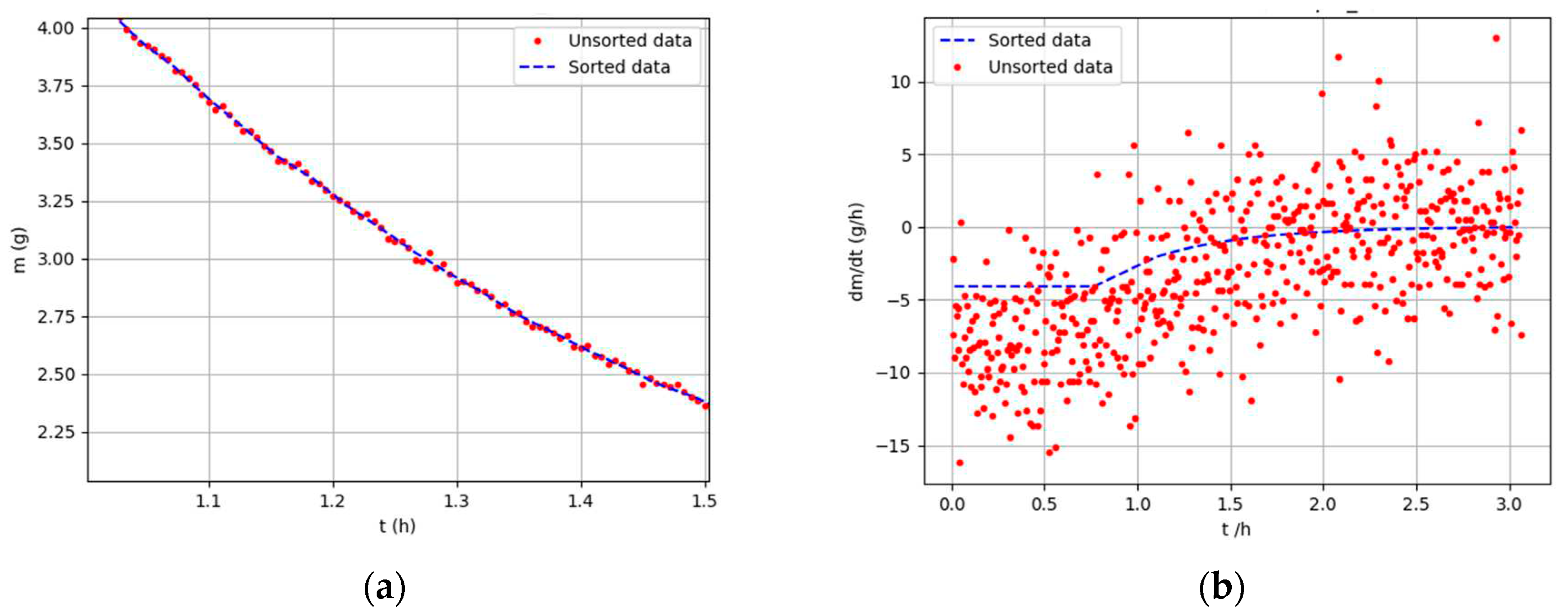
Figure 1 presents a comparison of sorted and unsorted mass data over time and the first mass derivative with respect to time.
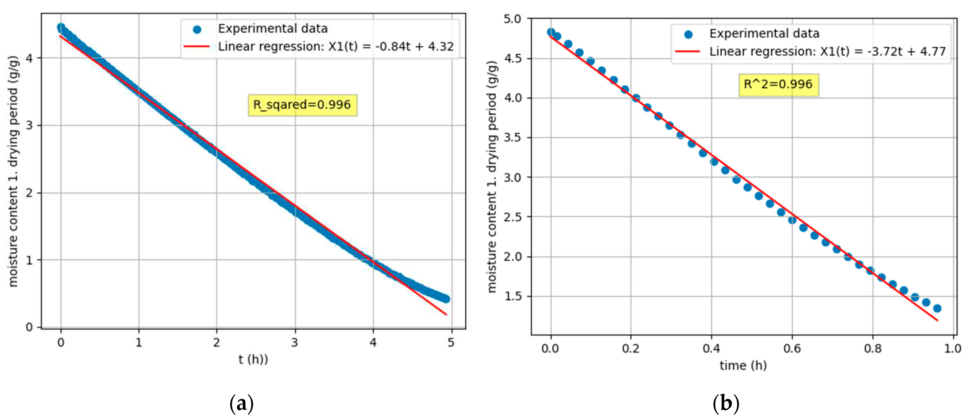
Stage 2: Linear regression of the first drying period
The first drying period, also known as the constant speed drying period, occurs at the beginning of the drying process when the drying speed is constant. During this period, there is sufficient moisture on the surface of the material and the evaporation rate is mainly determined by external conditions such as temperature, pressure, humidity and air-drying rate [
14]. Since the time dependence of the mass reduction is linear, the 1
st drying period can be given by eq 2:
In Stage 2, the program performs regression analysis on the experimental data from the first drying period, utilising the criterion R
2 > 0,99 to produce a linear function [
10].
The final data point chosen by the program in Stage 2 is the crucial drying point, defined by the coordinate X (, ), where represents the time of the critical point and is the free moisture at the critical point. This critical point marks the transition from the constant rate period to the falling rate period in the drying process.
Stage 3: Second drying period analysis
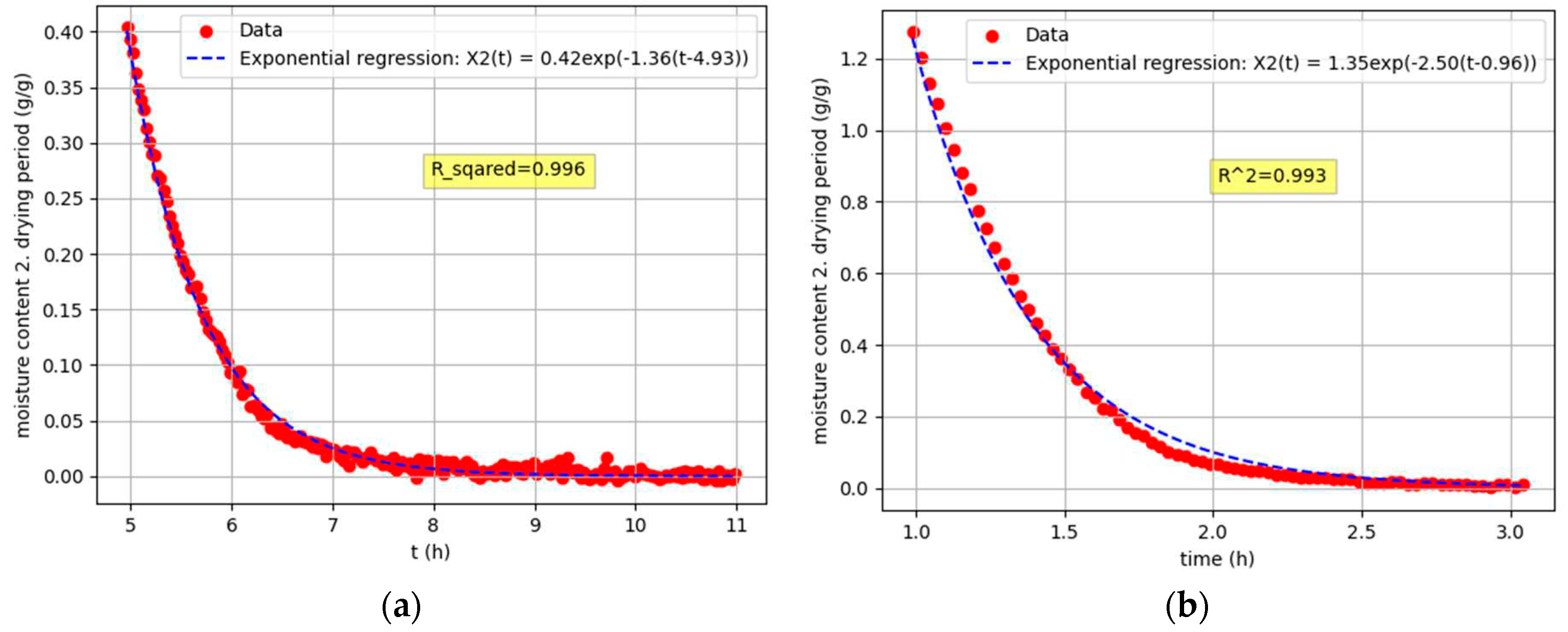
Stage 3 is based on the regression analysis of the experimental data obtained during the second drying period, which leads to an exponential function:
This function characterizes the final stage of the drying process, where the rate of drying decreases over time. The program determines the critical drying point, which is defined as the boundary where the linear function from Stage 2 ends and the exponential function from Stage 3 begins [
14].
The curve representing the second drying period follows an exponential function of the form of the eq 3. The exponential function captures the falling rate period of the drying process, as the rate of moisture loss decreases over time. In the following sections, we will delve deeper into the derivation and details of this exponential function, exploring its implications and applications in the context of drying processes.
Derivation of the second Drying Period’s Regression Function
To derive the regression function of the second drying period, it is necessary to first define the basic drying parameters as follows:
Where:
- moisture content of the substance (g g-1)
- mass of the sample, which varies with time (g)
- mass of the sample after drying (g)
This equation calculates the moisture content of the substance at any given time (
) relative to its initial moisture content (
). The moisture content decreases as the drying process continues [
14].
Where:
- free moisture content of the substance (g g-1)
- equilibrium moisture content at given constant drying conditions (g g-1)
Free moisture represents the amount of moisture in the substance that exceeds its equilibrium moisture content (
). During the constant-rate drying period, the free moisture is available for evaporation, and the drying process is typically limited by the external factors mentioned earlier [
14].
In our analysis, we assumed that the drying process during the second drying period can be characterized as quasi-stationary diffusion. Quasi-stationary diffusion refers to a scenario where the internal moisture diffusion within the material dominates the drying process, while external factors like surface evaporation and convective heat transfer have minimal influence. This assumption enables us to concentrate on the internal moisture transport mechanisms and simplifies the mathematical modeling of the drying process during the falling rate period. Quasi-stationary diffusion has been widely utilized in drying research to describe the behavior of different materials during the falling rate period [
14,
15,
16,
17,
18].
To derive a function describing the free moisture content of a material during the second drying period, we start with a simple mass balance equation, which states that the difference in water mass flow is equal to the accumulation:
The mass flow of water can be expressed as:
Where:
- mass flux of water (g s-1 m-2)
- molar mass of water (18 g mol-1)
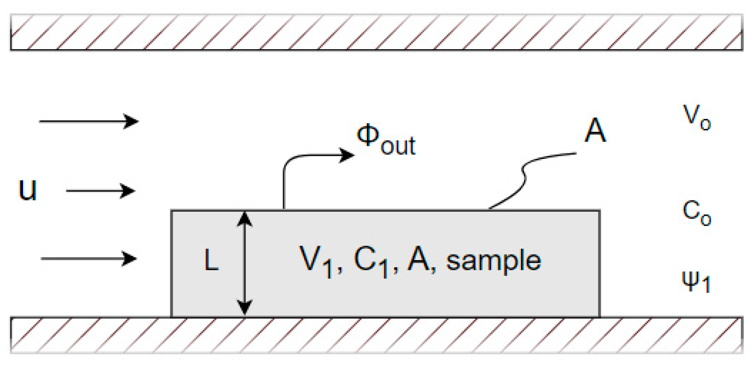
- surface area exposed to the drying air flow
Assuming that during the drying process, the mass flow of water originates exclusively from the material, therefore is
= 0, and the accumulation is equal to the change in mass over time. The water mass balance for the material system is:
Similarly, a mass balance of water can be derived for the air system, where it is assumed that all the mass of water is transferred from the material to the air.
is simplified as:
Assuming the concentration of water in the air remains constant, thus
= 0. The equations for the material and air systems are summed, rearranged, and the following is obtained:
Considering quasi-stationary diffusion and a thin film, the bulk flux can be approximated by:
Where:
- diffusion coefficient of water (m2 s-1)
- film thickness (m)
Combining the above equations yields a first-order differential equation:
Introducing a parameter k, where
, the solution to the differential equation at initial conditions
is:
Where:
- the critical time where the second drying period starts
- initial concentration of water in MSS
- concentration of water in the air
To determine how the moisture content of a substance,
varies with time, we express the water concentration as:
Combining the eq. 14 and 4:
Expressing C and obtaining:
Inserting the above equation into the previous one, we obtain:
Where:
- moisture content of water changing over time
- moisture content of water at point
- moisture content of water at infinite time
Subtracting the equilibrium humidity
from both sides of the eq. 18:
Considering the assumption that the humidity of a substance at infinite time
is equal to the equilibrium humidity
, the critical humidity is defined by:
Taking into account the above equation and the assumption, we can write the final equation describing the variation in free moisture content of the material during the second drying period as a function of time [
14,
15,
16,
17,
18]:
Stage 4: Calculating drying parameters
In Stage 4, the program calculates the drying parameters, which serve as key indicators for evaluating the efficiency and effectiveness of the drying process [
14].
These parameters are the following:
Where:
- the mass of dry matter (g)
- the drying rate (g m-2s-1)
- the area exposed to the drying air flow (m2)
Additionally, the program calculated the heat flux (q) according to the following eq.:
Where:
- heat flow (W)
- heat transfer coefficient (W m-2K-1)
- dry bulb temperature (K)
- wet bulb temperature (K)
Alternatively, q was calculated as:
Where:
- latent heat of vaporisation (kJ kg-1)
By rearranging the eq. 23 and 24, we can express the heat transfer equation as follows:
The mass flux (
) was calculated using the following equation:
Where:
- the molar mass of air (29 g mol-1)
- the mass transfer coefficient (mol m-2s-1)
- wet bulb humidity (g g-1)
- dry bulb humidity (g g-1)
From eq. 26 we can derive the mass transfer coefficient:
The literature frequently presents the mass transfer coefficient in units of m s
-1. To compute the coefficient in these units, the following expression should be used:
Where:
- mass transfer coefficient (m s-1)
- concentration of water at wet bulb temperature (mol L-1)
- concentration of water at dry bulb temperature (mol L-1)
An example of the derivation of the water vapour concentration equation is given by the example of the water vapour concentration at wet bulb temperature. The derivation of the dry bulb water vapour concentration is similar.
It is necessary to use the gas equation:
Where:
- Gas constant (8.314 J mol-1K-1)
- Partial vapour pressure at wet bulb temperature (kPa)
The partial pressure of water vapour can be expressed from the following equation [
14]:
Where:
- Atmospheric pressure (101,32 kPa)
Combine eq. 29 and 30 and highlight
:
To calculate the mass transfer coefficient in units of m s
-1, we combine eq. 28 and 31 and calculate
by analogy with
:
Once these parameters are determined, the program systematically logs and writes them to an Excel file for convenient data management and subsequent analysis [
14,
15,
16,
17,
18,
20]
Stage 5: Graph plotting
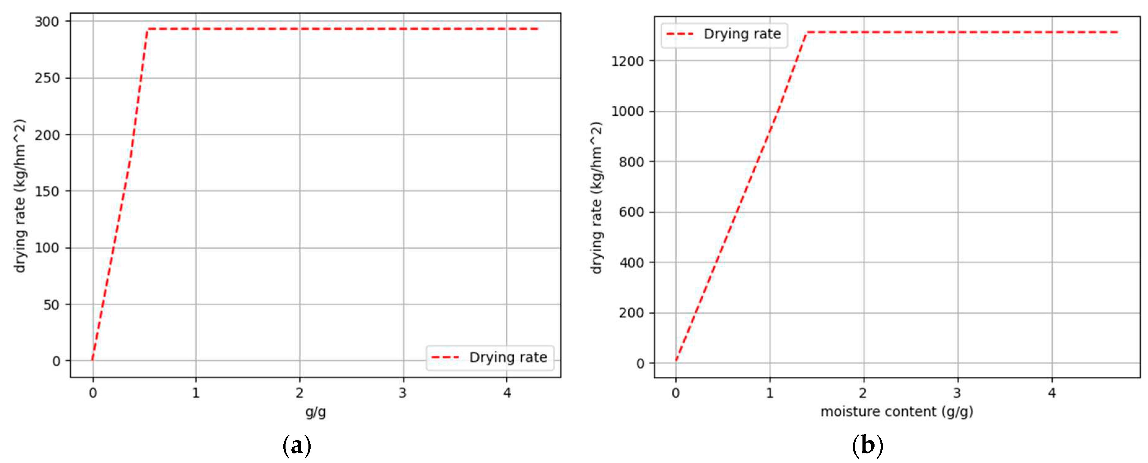
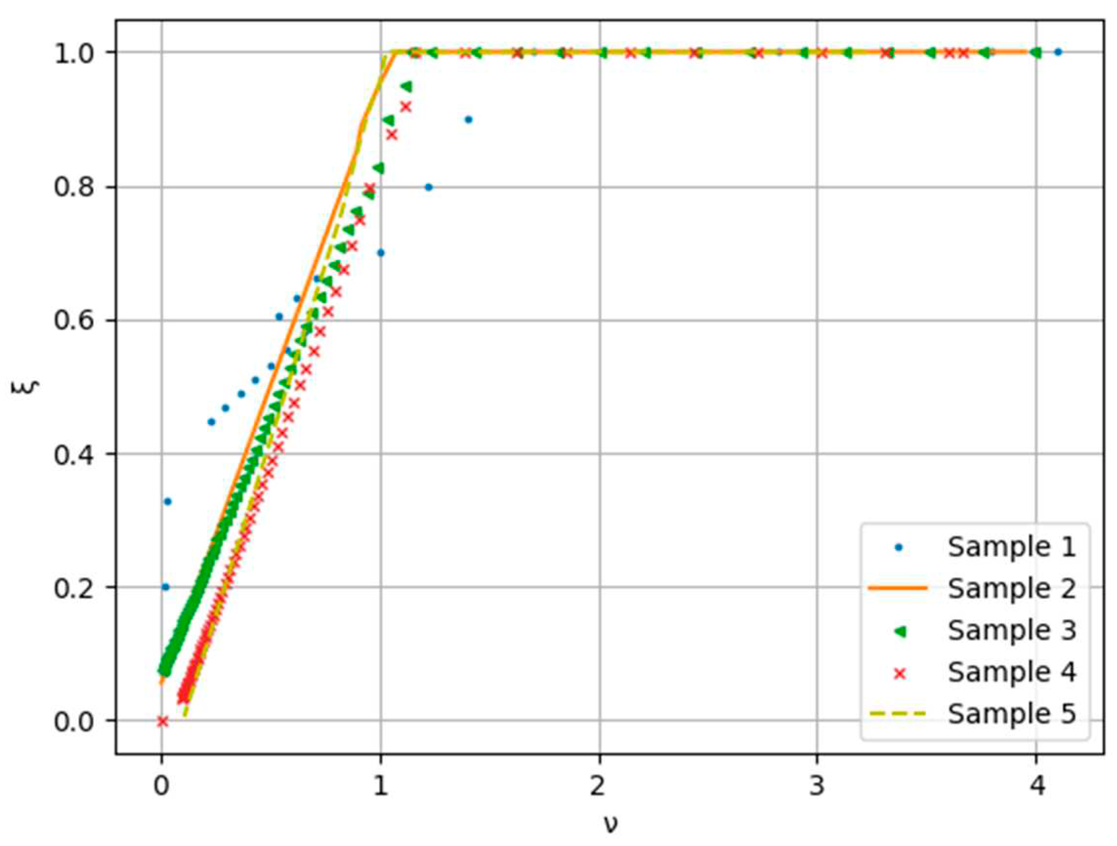
In stage 5, the program enhances data analysis by generating various diagrams. These include graphs that compare experimental and sorted data, plots of regression functions for the first and second drying periods against sorted data, and an overall drying curve plot that compares regression functions with experimental data. Additional diagrams depict the first derivative of humidity against time and the drying rate versus moisture content. Furthermore, a normalized drying rate curve is plotted using coordinates calculated using the following formulas [
19]:
Where:
- relative drying rate (dimensionless)
- characteristic moisture content (dimensionless)
These graphical representations enhance the comprehension of the drying process and can be applied at various temperature and air moisture conditions. [
14].
4. Conclusions
This study shows that the Python programming language is effective in analyzing and modelling chemical processes, particularly in the drying process. A successful analysis of drying data was accomplished using Python, and a program was created that could be beneficial in developing chemical processes yet on a laboratory scale. The significant drying parameters, such as the mass transfer coefficient, heat transfer coefficient, diffusion coefficient, drying rate, critical humidity, and critical drying time, were determined by the program. Furthermore, the research proves that Python is a suitable tool for modeling the drying process. The software analyzed the initial drying phase by utilizing a linear equation (eq. 2). It also automatically detects the point where the drying rate decreases, signifying the start of the second drying period. An exponential function (eq. 3), serving as a mathematical model, demonstrated exceptional conformity with the experimental data (R2 > 0,99) during this phase. Thereafter, a master curve for five different MSS samples was developed through analysis. This curve is instrumental in the planning of a drying process at different temperatures. This research showcases how Python can be a powerful tool for the analysis and modelling of chemical processes. The program devised in this research can be employed to draft and refine chemical procedures on an extensive scale. Moreover, the master curve can be utilized to blueprint the drying procedure under diverse temperatures. Furthermore, future investigations could enhance the precision of the master curve through the creation of a more advanced model or the inclusion of additional data from diverse MSS samples.
Figure 1.
Sorted vs. unsorted data: (a) mass change over time; (b) first derivative over time.
Figure 1.
Sorted vs. unsorted data: (a) mass change over time; (b) first derivative over time.
Figure 2.
Basic parameters of the drying process
Figure 2.
Basic parameters of the drying process
Figure 3.
Mass of MSS over time: (a); Sample 1, Tdry = 19,4 °C, Ψ = 33,6 % (b); Sample 5, Tdry = 52,4 °C, Ψ = 8,2 %.
Figure 3.
Mass of MSS over time: (a); Sample 1, Tdry = 19,4 °C, Ψ = 33,6 % (b); Sample 5, Tdry = 52,4 °C, Ψ = 8,2 %.
Figure 4.
Regression functions of the first drying period: (a); Sample 1, Tdry = 19,4 °C, Ψ = 33,6 %(b); Sample 5, Tdry = 52,4 °C, Ψ = 8,2 %.
Figure 4.
Regression functions of the first drying period: (a); Sample 1, Tdry = 19,4 °C, Ψ = 33,6 %(b); Sample 5, Tdry = 52,4 °C, Ψ = 8,2 %.
Figure 5.
Regression functions of the second drying period: (a); Sample 1, Tdry = 19,4 °C, Ψ = 33,6 %(b); Sample 5, Tdry = 52,4 °C, Ψ = 8,2 %.
Figure 5.
Regression functions of the second drying period: (a); Sample 1, Tdry = 19,4 °C, Ψ = 33,6 %(b); Sample 5, Tdry = 52,4 °C, Ψ = 8,2 %.
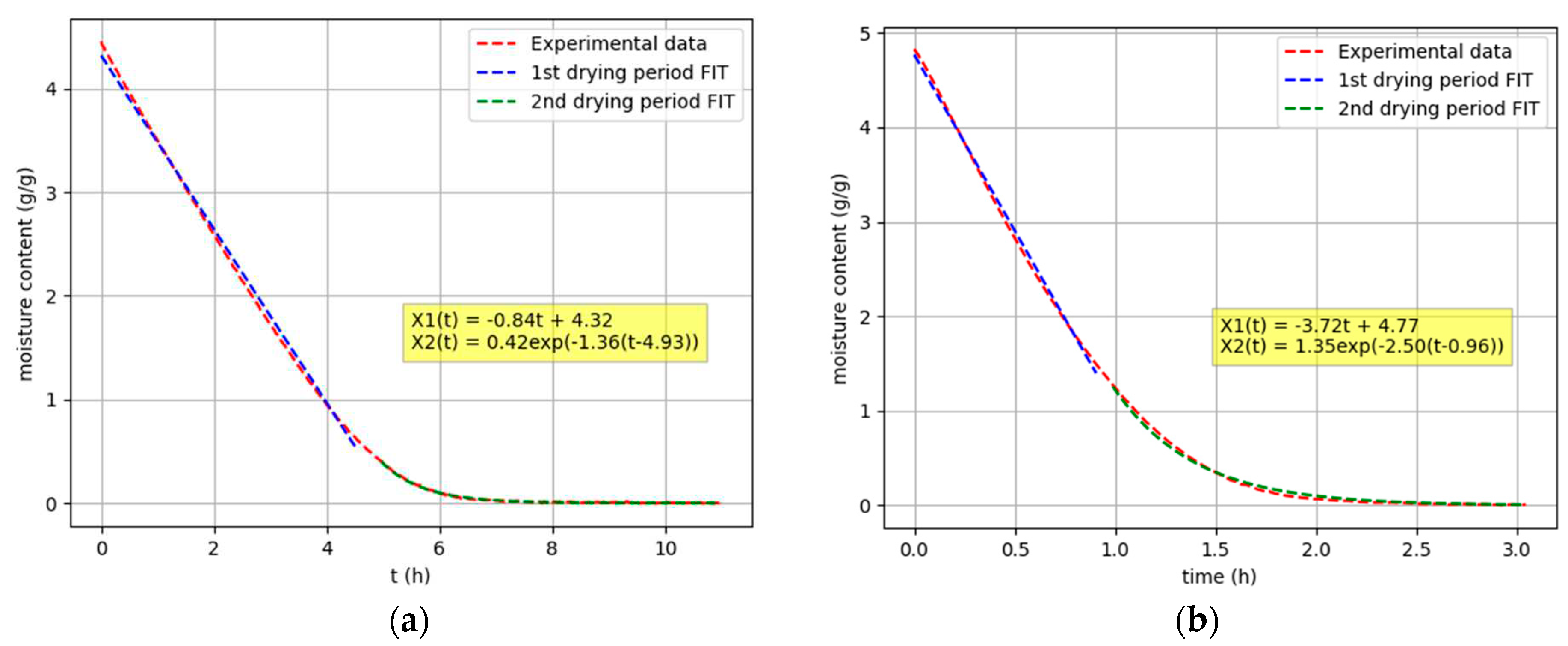
Figure 6.
Composite function of the first and second drying periods: (a); Sample 1, Tdry = 19,4 °C, Ψ = 33,6 %(b); Sample 5, Tdry = 52,4 °C, Ψ = 8,2 %.
Figure 6.
Composite function of the first and second drying periods: (a); Sample 1, Tdry = 19,4 °C, Ψ = 33,6 %(b); Sample 5, Tdry = 52,4 °C, Ψ = 8,2 %.
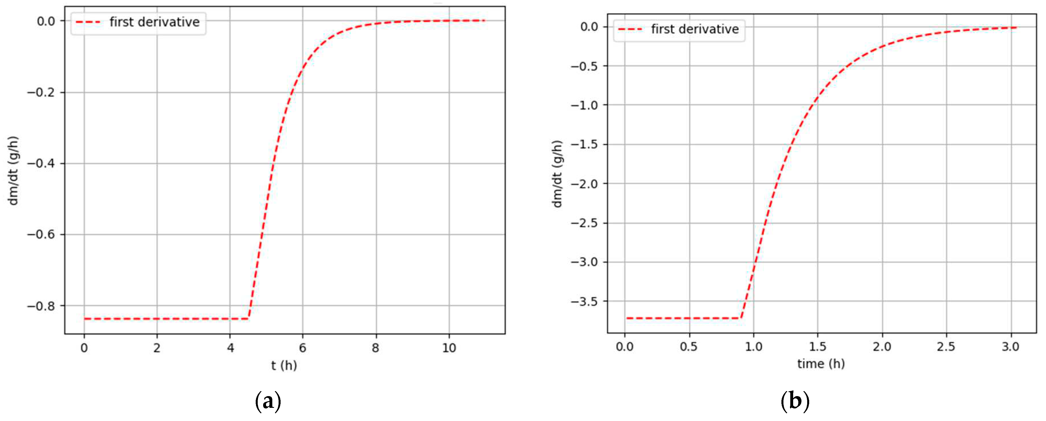
Figure 7.
First derivative functions: (a); Sample 1, Tdry = 19,4 °C, Ψ = 33,6 % (b); Sample 5, Tdry = 52,4 °C, Ψ = 8,2 %.
Figure 7.
First derivative functions: (a); Sample 1, Tdry = 19,4 °C, Ψ = 33,6 % (b); Sample 5, Tdry = 52,4 °C, Ψ = 8,2 %.
Figure 8.
Drying curves: (a); Sample 1, Tdry = 19,4 °C, Ψ = 33,6 % (b); Sample 5, Tdry = 52,4 °C, Ψ = 8,2 %.
Figure 8.
Drying curves: (a); Sample 1, Tdry = 19,4 °C, Ψ = 33,6 % (b); Sample 5, Tdry = 52,4 °C, Ψ = 8,2 %.
Figure 9.
Normalized drying rate curves.
Figure 9.
Normalized drying rate curves.
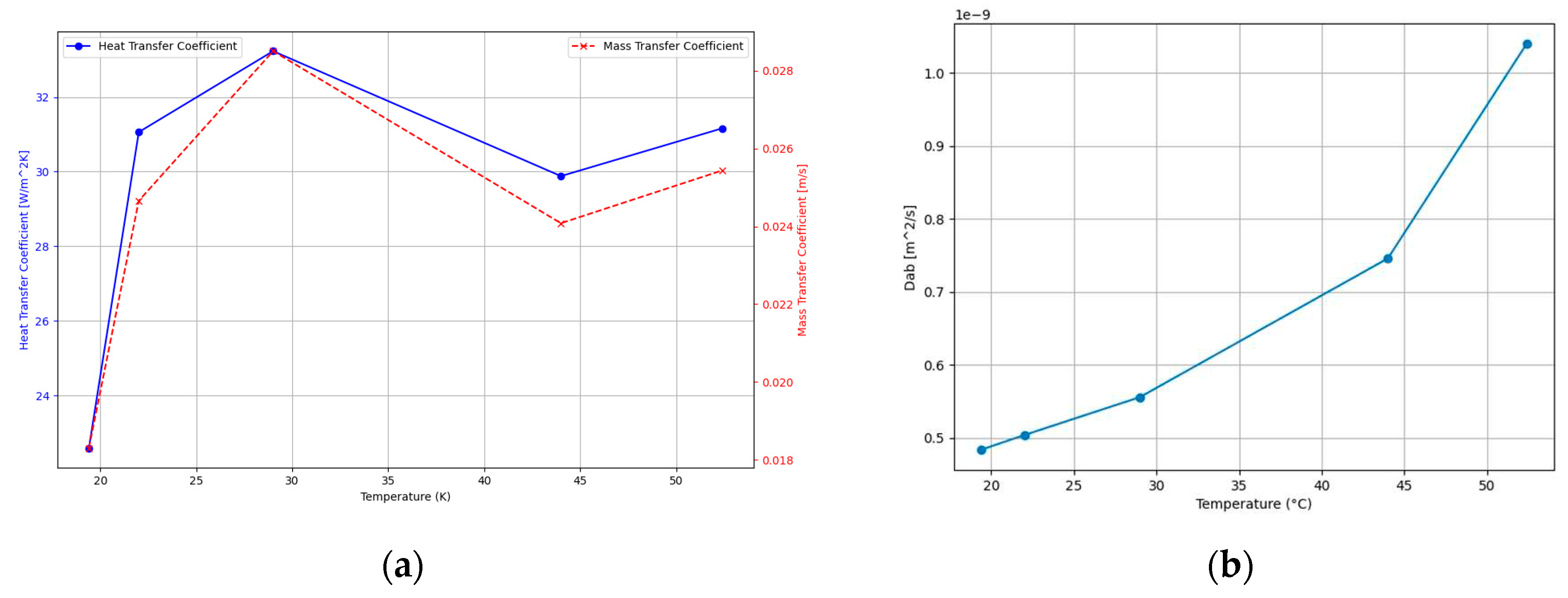
Figure 10.
programme-calculated drying parameters as a function of temperature: (a); heat transfer coefficient and mass transfer coefficient (b) diffusivity coefficient.
Figure 10.
programme-calculated drying parameters as a function of temperature: (a); heat transfer coefficient and mass transfer coefficient (b) diffusivity coefficient.
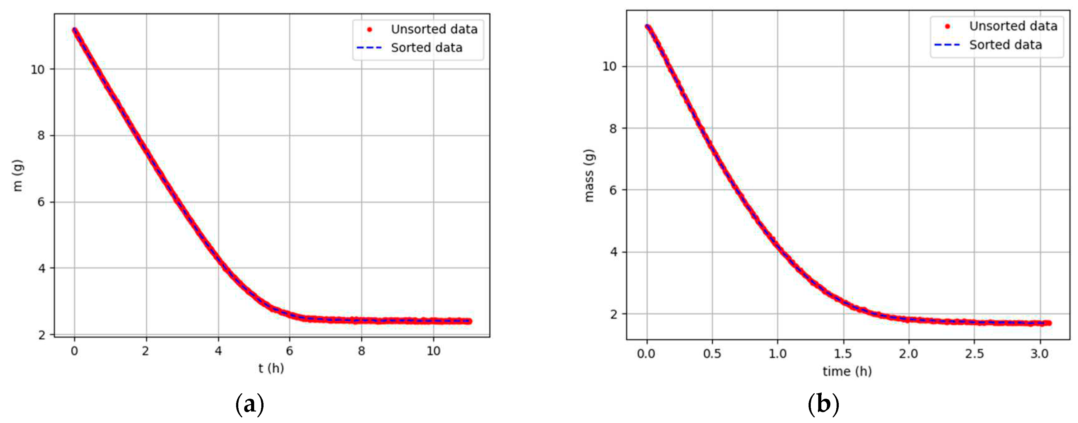
Figure 11.
Drying curves: (a); mass of MSS over time (b); regression function of first drying period.
Figure 11.
Drying curves: (a); mass of MSS over time (b); regression function of first drying period.
Table 1.
Measured data for sample 1 – 5.
Table 1.
Measured data for sample 1 – 5.
| Sample |
mMSS,start (g) |
mMSS,end (g) |
A [cm2] |
Tdry
[°C] |
Twet
[°C] |
Ψ
[%] |
Airspeed (m s-1) |
| 1 |
11,24 |
2,09 |
56,74 |
19,4 |
10,5 |
33,6 |
1,15 |
| 2 |
11,52 |
1,95 |
56,74 |
22,0 |
10,9 |
22,4 |
1,15 |
| 3 |
15,81 |
3,02 |
56,74 |
29,0 |
13,7 |
14,8 |
1,15 |
| 4 |
12,29 |
2,20 |
56,74 |
44,0 |
20,5 |
10,0 |
1,15 |
| 5 |
11,34 |
1,99 |
56,74 |
52,4 |
23,8 |
8,2 |
1,15 |
Table 2.
Programme calculated data for sample 1 – 5.
Table 2.
Programme calculated data for sample 1 – 5.
| Sample |
Na
[gs-1m-2] |
q
[W] |
h
[Wm-2K-1] |
[mol/m2s] |
[m s-1] |
Xcrit
[g g-1] |
tcrit
[h] |
Dab
[m2s-1] |
|
| 1 |
0,08 |
1,14 |
22,59 |
0,80 |
0,018 |
0,40 |
4,93 |
4,84E-10 |
|
| 2 |
0,14 |
1,96 |
31,06 |
1,07 |
0,025 |
1,07 |
2,60 |
5,04E-10 |
|
| 3 |
0,21 |
2,89 |
33,23 |
1,23 |
0,028 |
0,95 |
2,43 |
5,56E-10 |
|
| 4 |
0,29 |
3,99 |
29,88 |
1,01 |
0,024 |
1,22 |
1,35 |
7,46E-10 |
|
| 5 |
0,36 |
5,06 |
31,16 |
1,06 |
0,025 |
1,35 |
0,96 |
1,04E-09 |
|
