Submitted:
13 October 2023
Posted:
13 October 2023
You are already at the latest version
Abstract
Keywords:
1. Introduction
2. Acrobot control task
3. Neural networks
4. Training of neural networks by genetic algorithm
5. Experiment
6. Statistical test to compare GA with ES
7. Conclusion
- (1)
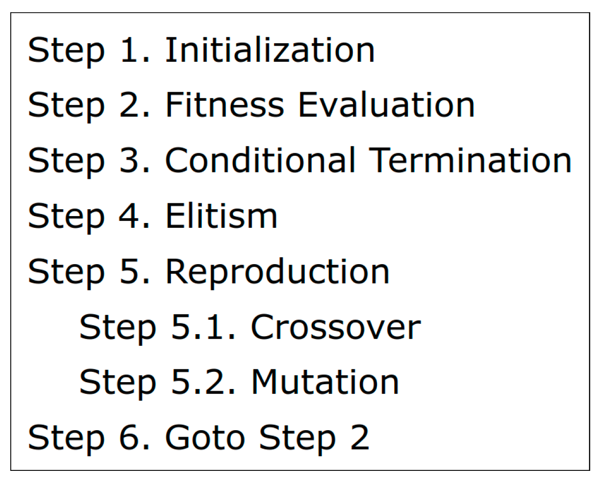
- In terms of the parameter settings for Genetic Algorithm, two approaches were employed: one with more generations and less offsprings (Table 2(a)), and the other with less generations and more offsprings (Table 2(b)). Based on the experimental results, it was observed that increasing generations significantly led to better solutions (p < .01). Interestingly, this result was opposite to that observed in the case of Evolution Strategy [15]. This indicates that the priority of generations and offsprings varies depending on the algorithm.
- (2)
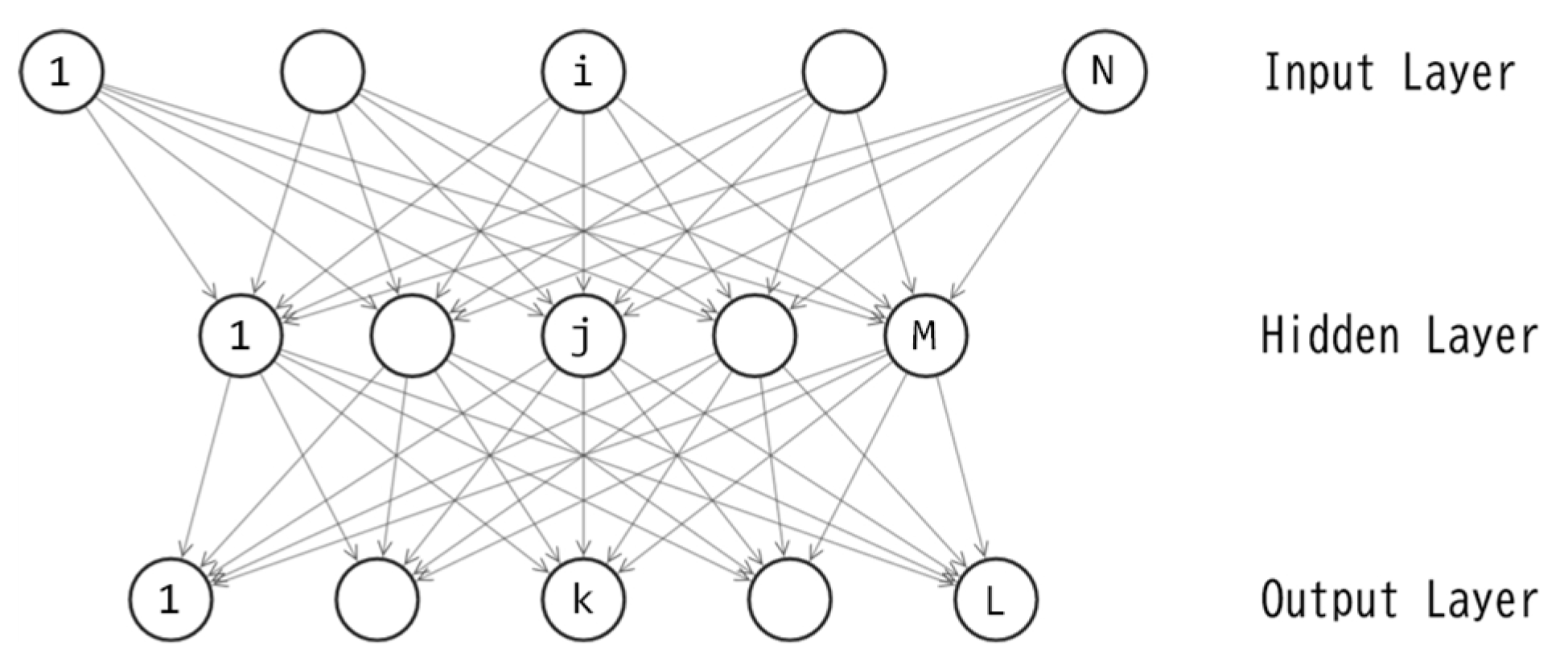
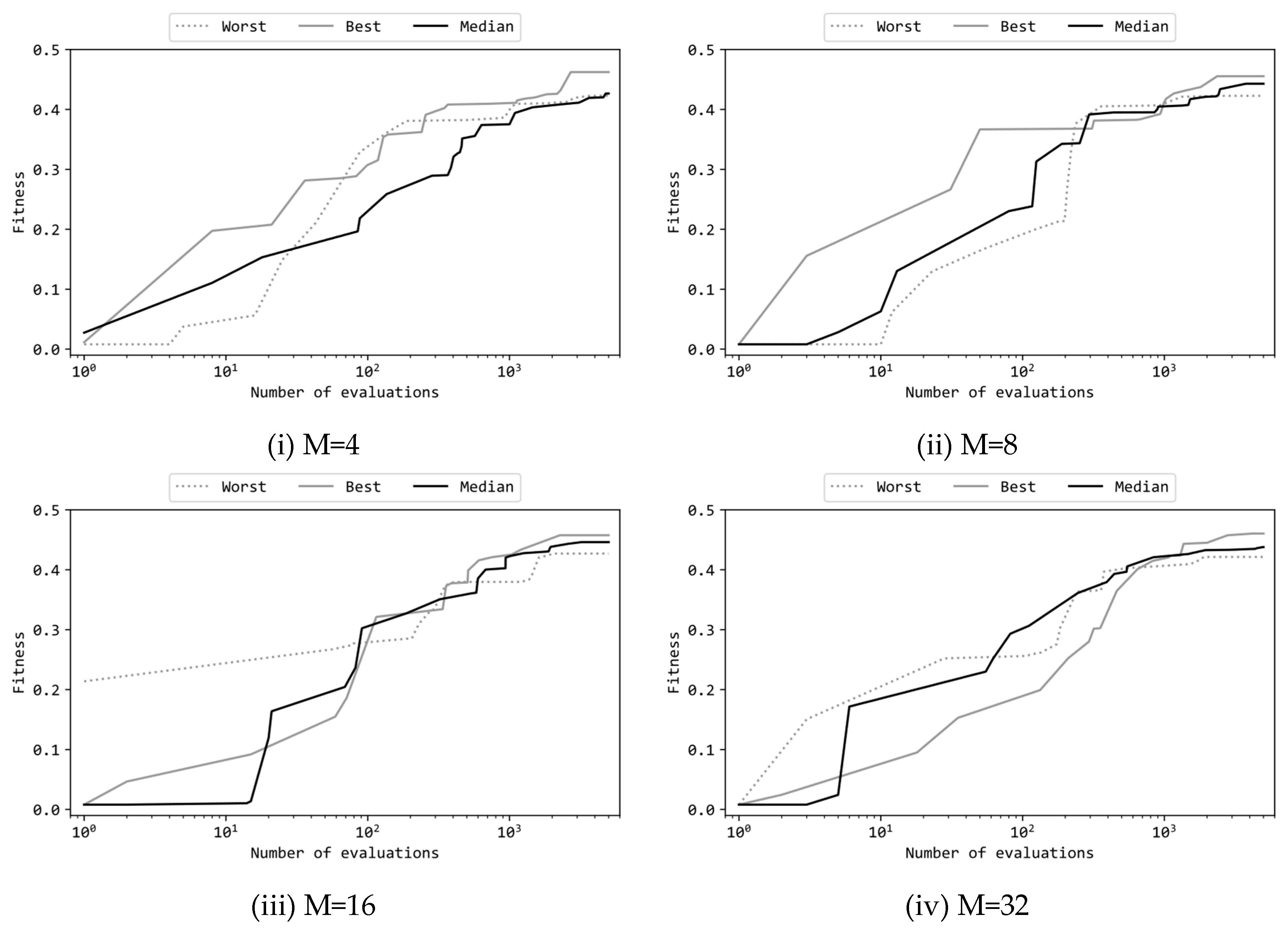
- Four different numbers of units in the hidden layer of the multilayer perceptron were compared: 4, 8, 16, and 32. The experimental results revealed that, in the case of 4 units, significantly inferior performance was obtained compared to the other three configurations. For 8 units, there was no statistically significant difference compared to 16 and 32 units. Therefore, from the perspective of the trade-off between performance and model size, 8 units in the hidden layer were found to be the optimal choice. This finding aligns with previous study using Evolution Strategy [15].
Acknowledgments
| 1 | |
| 2 | |
| 3 |
References
- Bäck, T., & Schwefel, H. P. (1993). An overview of evolutionary algorithms for parameter optimization. Evolutionary computation, 1(1), 1-23. [CrossRef]
- Fogel, D. B. (1994). An introduction to simulated evolutionary optimization. IEEE transactions on neural networks, 5(1), 3-14. [CrossRef]
- Bäck, T. (1996). Evolutionary algorithms in theory and practice: evolution strategies, evolutionary programming, genetic algorithms. Oxford university press.
- Eiben, Á. E., Hinterding, R., & Michalewicz, Z. (1999). Parameter control in evolutionary algorithms. IEEE Transactions on evolutionary computation, 3(2), 124-141.
- Eiben, A. E., & Smith, J. E. (2015). Introduction to evolutionary computing. Springer-Verlag Berlin Heidelberg.
- Schwefel, H. P. (1984). Evolution strategies: A family of non-linear optimization techniques based on imitating some principles of organic evolution. Annals of Operations Research, 1(2), 165-167. [CrossRef]
- Beyer, H. G., & Schwefel, H. P. (2002). Evolution strategies–a comprehensive introduction. Natural computing, 1, 3-52.
- Goldberg, D.E., Holland, J.H. (1988). Genetic Algorithms and Machine Learning. Machine Learning 3, 95-99. [CrossRef]
- Holland, J. H. (1992). Genetic algorithms. Scientific american, 267(1), 66-73.
- Mitchell, M. (1998). An introduction to genetic algorithms. MIT press.
- Sastry, K., Goldberg, D., & Kendall, G. (2005). Genetic algorithms. Search methodologies: Introductory tutorials in optimization and decision support techniques, 97-125.
- Storn, R., & Price, K. (1997). Differential evolution–a simple and efficient heuristic for global optimization over continuous spaces. Journal of global optimization, 11, 341-359. [CrossRef]
- Price, K., Storn, R. M., & Lampinen, J. A. (2006). Differential evolution: a practical approach to global optimization. Springer Science & Business Media.
- Das, S., & Suganthan, P. N. (2010). Differential evolution: A survey of the state-of-the-art. IEEE transactions on evolutionary computation, 15(1), 4-31. [CrossRef]
- Okada, H. (2023). Evolutionary reinforcement learning of neural network controller for Acrobot task – Part1: evolution strategy. Preprints.org, doi: 10.20944/preprints202308.0081.v1.
- Rumelhart, D. E., Hinton, G. E., & Williams, R. J. (1986). Learning internal representations by error propagation. Parallel distributed processing: explorations in the microstructure of cognition, vol. 1: foundations. MIT Press, Cambridge, MA, USA, 318-362.
- Collobert, R., & Bengio, S. (2004). Links between perceptrons, MLPs and SVMs. In Proceedings of the twenty-first international conference on Machine learning (ICML 04). Association for Computing Machinery, New York, NY, USA, 23. [CrossRef]
- Eshelman, L.J. & Schaffer, J.D. (1993). Real-coded genetic algorithms and interval-schemata, Foundations of Genetic Algorithms, 2, 187-202. [CrossRef]
- Okada, H. (2023). An evolutionary approach to reinforcement learning of neural network controllers for pendulum tasks using genetic algorithms, International Journal of Scientific Research in Computer Science and Engineering, 11(1), 40-46.


| Hyperparameters | (a) | (b) |
|---|---|---|
| Number of offsprings () | 10 | 50 |
| Generations | 500 | 100 |
| Fitness evaluations | 10500=5,000 | 50100=5,000 |
| Number of elites (E) | 100.2=2 | 500.2=10 |
| for blend crossover | 0.5 | 0.5 |
| Mutation probability | 1/D | 1/D |
| M | Best | Worst | Average | Median | |
|---|---|---|---|---|---|
| (a) | 4 | 0.462 | 0.423 | 0.433 | 0.427 |
| 8 | 0.455 | 0.423 | 0.442 | 0.443 | |
| 16 | 0.458 | 0.427 | 0.443 | 0.446 | |
| 32 | 0.460 | 0.421 | 0.441 | 0.438 | |
| (b) | 4 | 0.452 | 0.398 | 0.428 | 0.432 |
| 8 | 0.434 | 0.407 | 0.421 | 0.426 | |
| 16 | 0.435 | 0.382 | 0.416 | 0.422 | |
| 32 | 0.418 | 0.396 | 0.408 | 0.410 |
Disclaimer/Publisher’s Note: The statements, opinions and data contained in all publications are solely those of the individual author(s) and contributor(s) and not of MDPI and/or the editor(s). MDPI and/or the editor(s) disclaim responsibility for any injury to people or property resulting from any ideas, methods, instructions or products referred to in the content. |
© 2023 by the authors. Licensee MDPI, Basel, Switzerland. This article is an open access article distributed under the terms and conditions of the Creative Commons Attribution (CC BY) license (http://creativecommons.org/licenses/by/4.0/).


