A Global Resource Scheduling for Distributed Edge Computing

Preprint

Article

A Global Resource Scheduling for Distributed Edge Computing

Altmetrics

Downloads

Views

Comments

A peer-reviewed article of this preprint also exists.

Aiping Tan

,Yunuo Li,

Yan Wang^*,Yujie Yang

Aiping Tan

,Yunuo Li,

Yan Wang^*,Yujie Yang

This version is not peer-reviewed

Submitted:

12 October 2023

Posted:

13 October 2023

You are already at the latest version

Alerts

Abstract

Recently, there has been a growing interest in distributed edge computing resource scheduling. For example, application scenarios such as intelligent traffic systems and Internet of Things(IoT) intelligent monitoring require the scheduling and migration of distributed resources. Distributed resource scheduling needs to consider the cost of resource scheduling, with the primary goal of finding the optimal strategy among various feasible solutions. There are different definitions for optimization objectives in different application scenarios, such as cost, transmission delay, energy consumption, etc. Current research mainly considers the optimization problem of local resource scheduling but needs more consideration of global resource scheduling. This paper defines a global resource scheduling problem for distributed edge computing and proves that the problem is NP-Hard. A heuristic solution strategy based on the Ant Colony Algorithm(ACO) was proposed, and Particle Swarm Optimization(PSO) was used to optimize the parameters of the ACO. Finally, an experimental comparative analysis was conducted to demonstrate that the algorithm proposed in this paper has good accuracy and iteration cost performance.

Keywords:

Subject: Computer Science and Mathematics - Data Structures, Algorithms and Complexity

1. Introduction

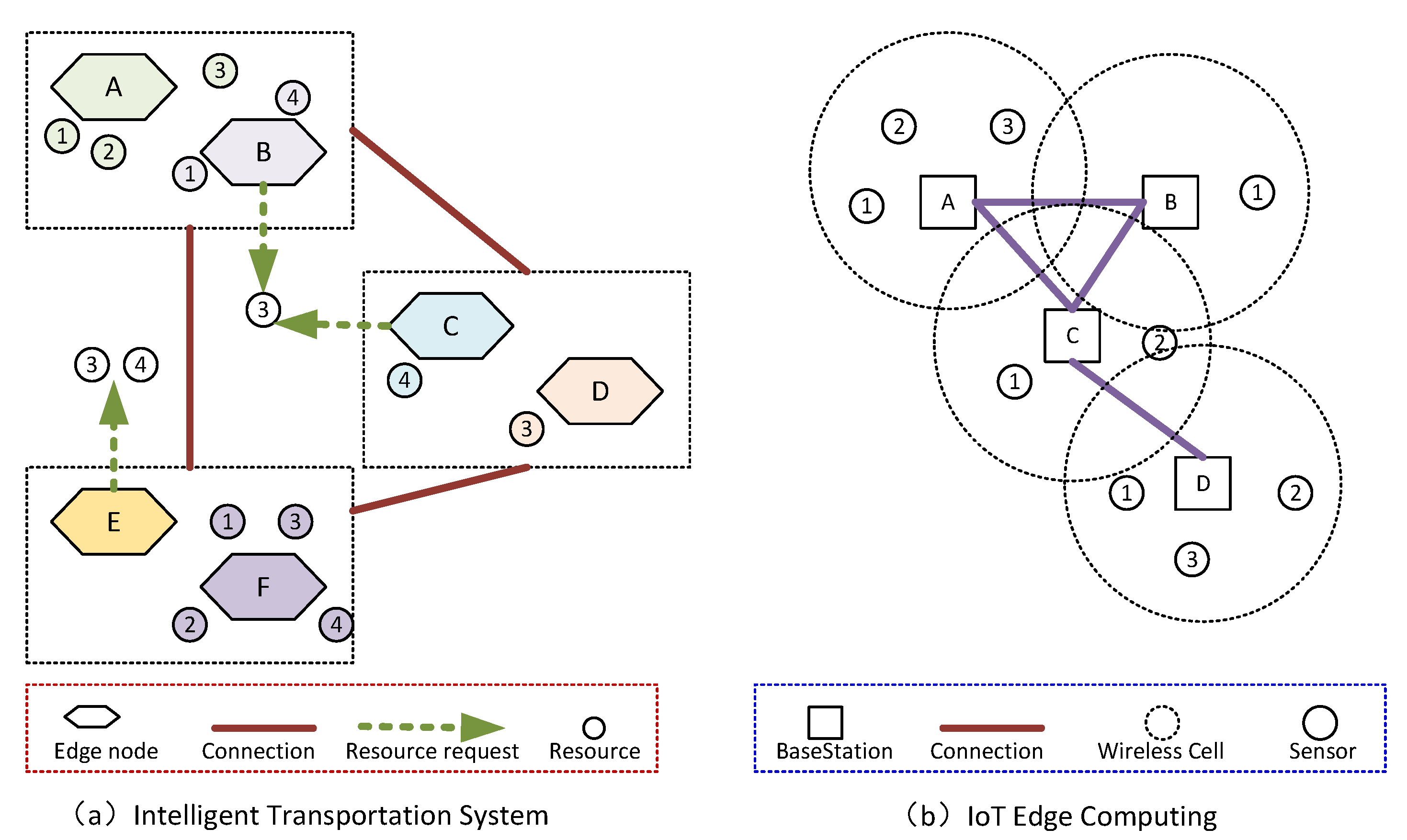
The resource scheduling of distributed edge computing has an extensive range of applications. For example, Figure 1(a) shows an application case of an intelligent transportation system. Different edge computing nodes are scattered in other regions to monitor local traffic resources, such as traffic police, rescue vehicles, ambulances, etc., and make real-time resource scheduling requests according to traffic conditions. In Figure 1(a), node B and node C require resource 3, and there are multiple feasible options for selecting the appropriate allocation to node B and C among the nodes with resource 3. Therefore, scheduling the resource situation of all nodes from a global perspective is a problem worth studying. This problem requires minimizing the scheduling cost while ensuring that the requirements of all nodes are met. Figure 1(b) shows a case of edge computing of the Internet of Things(IoT). Base station A receives data from sensors 1, 2, and 3, then selects the base station where the corresponding target sensor is located to achieve data forwarding. For example, to which target base station should sensor 1 data from base station A be migrated? From a global perspective, ensuring the minimum latency while all data is migrated is significant.

Some scholars have started large-scale, distributed resource migration and dispatching research based on different application scenarios[1,2,3]. Jia et al.[4] have proposed a two-layer Distributed Collaborative Evolution (DCE) architecture with adaptive computing resources for large-scale optimization. Experimental studies have shown that the distributed architecture proposed has high scalability and efficiency. Askarizade et al.[5] use virtualization technology to apply hybrid technology to resource management through virtualization technology. This technology uses the K average cluster to the mapper and a micro-genetic algorithm to improve the ramming method. The research found that the KMGA technology can effectively reduce data centers in the data center. Energy consumption and continuous service quality provide a good compromise. In addition, compared with Particle Swarm Optimization(PSO) and genetic algorithms similar to hybrid technology, it minimizes virtual machine migration’s number and generation time. Yuan et al.[6] have established an intelligent manufacturing workshop resource dispatch model. Improved Non-dominating Sorting Genetic Algorithms (NSGA-II), selected evaluation functions based on sorting levels and congestion, and introduced a competitive mechanism. A new generation of groups is generated based on process and machine-based random mutation strategies and cross-methods. The elite retention strategy was improved, the variable proportional method was designed to determine the probability, and the layered analysis method decided the optimal solution. The superiority and effectiveness of the improvement algorithm were verified through the test of the benchmark cases and actual production and processing problems. There are still some problems in existing research, which are mainly reflected in the following: first, the existing research has relatively little research on global optimization; second, the optimization goals are single, usually only certain factors such as delay and energy consumption; third, in the process of optimization, lack of consideration of dynamic change parameters.

Given the shortcomings of existing research, this paper defines a global resource scheduling problem for distributed edge computing, analyzes the computational complexity of this problem, and proposes a solution algorithm. The main contributions of this article are as follows:

(1) The global resource scheduling problem of distributed edge computing is defined. Firstly, the designed objective function includes two optimization objectives: the first is resource price, and the second is the cost of migration. Secondly, the constraints of the problem were described. Firstly, all resource requests should be satisfied, and secondly, the scheduling results must meet the price budget of the resource requests. Finally, it is proven that the problem is NP-hard.

(2) Due to the difficulty in finding practical polynomial time algorithms for the NP-Hard problem, this paper proposes an adaptive dynamic scheduling algorithm based on Ant Colony Optimization(ACO). ACO has a fast convergence speed and is not easily trapped in local optimal solutions. However, the performance of this method is limited by parameter settings, and ACO has many parameters, making it difficult to set appropriate parameter combinations manually. Therefore, this article utilizes PSO to optimize parameters during the ACO process, making the parameter settings for each iteration more reasonable.

(3) Compare and analyze the proposed algorithm with existing methods through experiments, including the primary ACO, Genetic Algorithm(GA), and ACO-GA hybrid algorithm. Compare and analyze algorithm performance for accuracy and iteration cost.

The remaining work of this article is as follows: Section 2 introduces the relevant research work of this article. Section 3 defines the global resource scheduling problem and analyzes its computational complexity. Section 4 proposes an adaptive dynamic scheduling algorithm based on the ant colony algorithm and utilizes particle swarm optimization for parameter optimization. Section 5 builds an experimental platform and conducts a comparative analysis of algorithm performance. Section 6 summarizes the work of this article.

2. Related work

At present, the research direction of distributed resource scheduling is comprehensive, mainly including network data flow scheduling[7], cloud computing[8], language processing[9], energy scheduling[10], blockchain[11] and other fields.

(1) Resource scheduling

Shen et al.[12] transformed the multi-virtual machine scheduling problem into a new structured combinatorial optimization problem. It is a reinforcement learning problem. Moreover, they proposed a reinforcement learning algorithm with an incremental reward scheme and scenario-guided sampling strategy. In [13], the regional optimization of the irrigation plan is realized by combining the multi-objective algorithm with the exponential efficiency coefficient method. In [14], several optimization attributes are proposed based on the characteristics of high-end equipment development, and an effective heuristic algorithm is designed. Since the resource-constrained project scheduling problem is an NP-Hard problem, three neighborhoods of the problem are constructed, and a variable neighborhood search algorithm is developed to solve the problem. Wu et al.[15] studied the existing issues in the employee evaluation mechanism of enterprises. Improved the current evaluation model based on neural network and analytic hierarchy process, and scientifically and effectively evaluated the matching degree of employees’ abilities and job requirements by learning the RBF neural network model to achieve the best matching and migration of employees and jobs. Yuan et al. [16] studied the scheduling method of dynamic service resources in a cloud manufacturing environment. This method aims at the time, cost, quality, and capacity and establishes an optimal scheduling model for emotional service resources. The ACO is improved, and the GA functions are used to optimize the objective function. The GA-based optimization fusion algorithm is proposed to solve the model. Wang et al. [17] proposed a distributed PSO method and extended it to large-scale cloud workflow scheduling. This method divides the whole population into multiple groups. It uses the master-slave multi-group distributed model to co-evolve these groups to form a Distributed PSO (DPSO) to enhance the diversity of the algorithm. DPSO adopts Dynamic Group Learning (DGL) strategy to balance diversity and convergence. Jiang et al. [18] proposed a Distributed Intelligent Resource Scheduling (DIRS) framework to minimize the sum of task delay and energy consumption. The scheduling problem can be expressed as a mixed integer nonlinear programming. Maab et al. [19] proposed an intelligent meta-heuristic optimization model to solve the problem of low quality of service and realized the optimization of time and precision in task unloading through the PSO on GPU. Zhang et al. [20] proposed a coevolutionary algorithm with Function-Independent Decomposition (FID). For large-scale problems, the binary code of the original model is converted to integer code to reduce the dimension, and a new FID is designed to decompose the problem effectively.

(2) Routing scheduling

The research of routing scheduling has a wide range of engineering applications[21], such as urban vehicle scheduling, robot path planning in intelligent factories, etc. Jahic et al. [22]proposed a scheduling model for urban bus charging. The model considers a heterogeneous fleet of electric buses with different battery capacities. The optimized scheduling method minimizes the number of buses charged simultaneously, reducing the peak load. Li et al. [23] proposed a time scheduling method for fixed line-oriented urban bus departure. It is proved that the scheduling problem is NP-hard, simplified as a variant of a k-clustering problem, and a practical application of dynamic programming. Mousa et al. [24] proposed parallelizing particle swarm optimization based on a graphics processing unit (GPU) to balance the cluster size and identify the shortest path.

(3) Network scheduling

Agiwal et al. [25] studied the current 4G-5G interworking solutions, analyzed the practical application feasibility and challenges of various interworking solutions, discussed the possibility of spectrum sharing between 4G and 5G wireless networks, and discussed the path of migration to 5G independent networks. Son et al. [26] proposed a dynamic resource allocation algorithm for Virtual Network Functions (VNFs). The algorithm considers the latency requirements of different applications in the service function chain. It allows delay-sensitive applications to reduce end-to-end network latency through edge resources. Zhao et al. [27] proposed an adaptive distributed scheduling algorithm on resource-constrained edge clusters of the Internet of Things. The algorithm uses the Convolution Neural Network(CNN) to optimize the distributed resource scheduling problem and uses the minimum memory occupation as the objective function. This method adopts a new work scheduling process to improve data reuse and reduce overall execution delay.

In summary, the current research has involved many fields, including intelligent grid [28], smart mining[29], smart factory[30], etc. However, most current research focuses on a single optimization goal, such as the minimum delay, the shortest path, etc. Different engineering application scenarios have other problems, and their solution methods differ. Therefore, the optimization method should be designed according to specific requirements.

3. System formulation

3.1. Problem definition

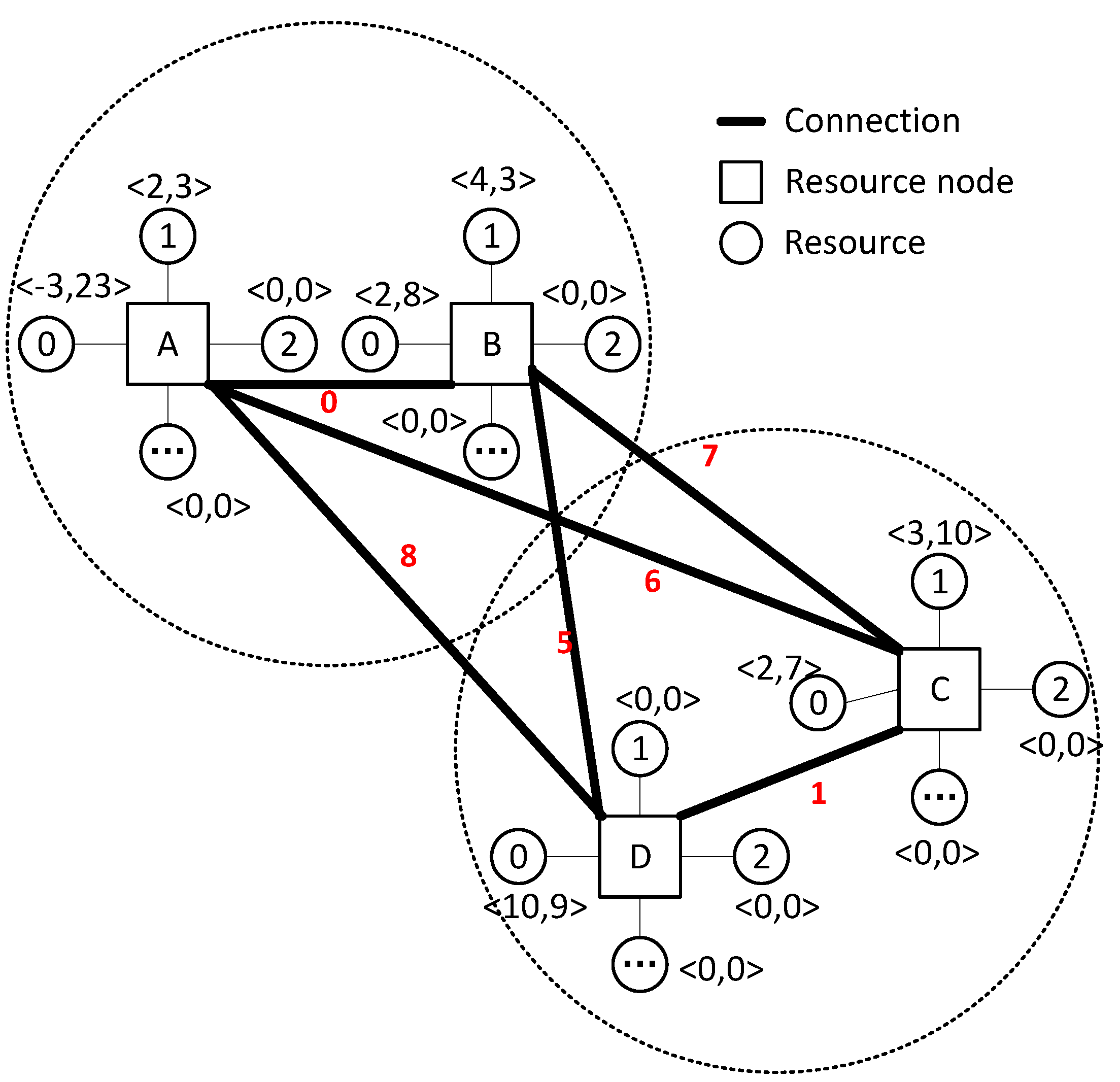
Figure 2 shows the topology of the system. Each resource node in the figure can represent any entity that owns resources, such as an intelligent edge node or IoT base station in Figure 1. Each resource node has multiple resources of the same type, and each resource has two key attributes

〈C, P〉

. Where C represents the number of resources, the entity owns C resources if it is a positive number. The entity must request at least C resources if it is zero or negative. P represents the resource price. If

C > 0

, then P represents the unit price of the resource. If

C \leq 0

, P represents the total resource budget requested. The weight value of the edge between any two nodes represents the contribution value of resource migration between these two nodes. It mainly reflects the distance between nodes, migration history, and other information. This value will be automatically updated with each node resource migration. As shown in Figure 2, nodes A and B are in the same cell, represented by dotted lines. It shows that the distance cost of resource migration between these two nodes (in other applications, such as edge computing of the Internet of Things, which can represent the communication cost) is relatively small. If node A requires at least 3 No.0 resources, the total budget is 23. Three nodes, B, C, and D, have No.0 resources. The unit price of node D is 9, and node B is 8. If three resources are obtained from D or B, we have

3 \times 9 > 23

and

3 \times 8 > 23

, which are not as expected. Therefore, only one part can be selected from D and B. In this example, there are many options, such as migrating 2 No.0 resources from B and 1 No.0 from C, so the total price is

2 \times 8 + 1 \times 7 = 23

, which meets the budget requirements. Similarly, we can migrate 1 No.0 resource from B, C, and D, respectively, so the total price is

8 + 7 + 9 = 24

. With the increase in the number of nodes and resource types, when there are multiple nodes migrating resources, how to ensure the minimum scheduling cost of each node is a challenging global optimization problem.

Suppose there are I nodes in total, and each node has the same J resource type.

\forall i \in \{0, 1, \dots, I - 1\}, j \in \{0, 1, \dots, J - 1\}

C_{i, j}

represents the quantity of the j-th resource of the i-th node;

P_{i, j}

represents the unit price of the j-th resource at the i-th node.

\forall i, i^{'} \in \{0, 1, \dots, I - 1\} \land i \neq i^{'}

L_{i, i^{'}}

represents the migration cost between node i and node

i^{'}

. Suppose maxP and maxL are used to represent the upper limit of resource unit price and migration cost; then the Quality of Service(QoS) function of node i requests

i^{'}

migration resource j is shown as follows:

Q_{i, i;} (j) = \frac{1}{\frac{X_{i, i^{'}} (j) \times P_{i^{'}, j}}{maxP} \times α + \frac{L_{i, i^{'}}}{maxL} \times (1 - α)}

(1)

Where

α

is a balance factor used to set the importance of price and migration cost according to user needs. Where

X_{i, j} (j)

represents the number of resource j migrated from node j to node i.

L_{i, i^{'}}

is not fixed. It includes the migration distance between nodes i and

i^{'}

, historical migration records, etc. After each migration, we can modify the value of

L_{i, i^{'}}

according to the results of the previous migration. The modification principles can be determined according to the actual situation in specific engineering applications. For example, for the edge computing scenario of intelligent transportation, if the last scheduling effect between two edge nodes is good,

L_{i, i^{'}}

can be increased; otherwise, it can be reduced.

3.2. Computational complexity analysis

For given

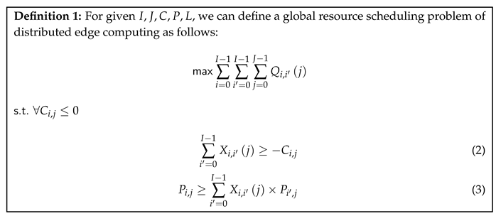
I, J, C, P, L

, we use

S (I, J, C, P, L)

to represent the solution function of the global resource scheduling problem of distributed edge computing. We have the following theorem:

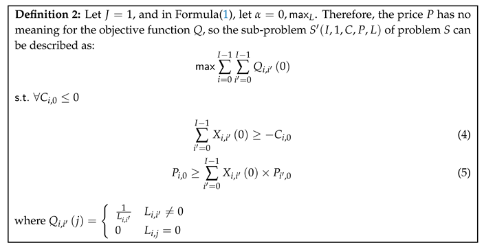
Let us prove theorem 1. According to definition 1, we define sub-problem

S^{'}

of problem S:

We have the following theorem:

Proof:

To prove theorem 2, we need to find a known NP-C problem and then prove that the problem can be reduced to problem

S^{'}

. A 0-1 knapsack problem is proposed and proved to be an NP-C problem[31].

For given N items and knapsack capacity X, we use the function

G (N, K, w, v)

to represent the 0-1 knapsack problem. For problem G, any input

N, K, w, v

, we will convert it to the input of

S^{'}

; the principle is as follows:

We need to prove that the same output can be obtained for questions G and

S^{'}

1: Suppose that the problem $S^{'}$ gets an output result X satisfying definition 2. Since only $C_{0, 0} \leq 0$ , we only consider $X_{0, i^{'}} (0)$ . Therefore, $\forall i^{'} \in \{1, \dots, I - 1\}$ , let $x [i^{'} - 1] = X_{0, i^{'}} (0)$ . According to formula() of definition 2, we have $P_{0, 0} \geq \sum_{i^{'} = 0}^{I - 1} X_{0, i^{'}} (0) \times P_{i^{'}, 0}$ . See in the input conversion principle(★), we have $K \geq \sum_{i^{'} = 1}^{I - 1} x [i^{'} - 1] \times w [i^{'} - 1]$ . Since $I = N + 1$ , we have $K \geq \sum_{i^{'} = 0}^{N - 1} x [i^{'}] \times w [i^{'}]$ , which satisfies the formula(6) of definition 3. Therefore, the output of question $S^{'}$ can be transformed into the output of question G. $(▪)$
2: Suppose that the problem G gets an output result x satisfying definition 3. $\forall i \in \{0, 1, \dots, N - 1\}$ , let $X_{0, i + 1} (0) = x [i]$ . According to formula(6), we have $\sum_{i = 0}^{N - 1} x [i] \times w [i] \leq K$ . See in the input conversion principle(★), we have $\sum_{i = 0}^{N - 1} X_{0, i + 1} (0) \times P_{i + 1, 0} \leq P_{0, 0}$ . Due to $I = N + 1$ , we have $\sum_{i = 1}^{I - 1} X_{0, i} (0) \times P_{i, 0} \leq P_{0, 0}$ . Because only $C_{0, 0} = 0$ , we have $\sum_{i^{'} = 0}^{I - 1} X_{0, i^{'}} (0) \geq 0 = - C_{0, 0}$ satisfying formula(4)definition 2. Therefore, the output of question G can be transformed into the output of question $S^{'}$ . $(▪ ▪)$

In conclusion,

(▪)

and

(▪ ▪)

indicate that problem G and

S^{'}

have the same output. Because the input conversion process of

(★)

is completed in polynomial time, theorem 2 holds!

Since it has been proved that

S^{'}

is an NP-hard problem, the more complex problem S must be an NP-hard problem. Theorem 1 holds.

4. Algorithm design

4.1. Design of heuristic algorithm based on ACO

Since problem S has been proven NP-Hard, we choose a heuristic algorithm to solve this problem. In the heuristic algorithm, this paper chooses the ACO to design.

The ACO is an intelligent heuristic algorithm. It solves some optimization problems by simulating the process of ants’ foraging in nature. In the whole search process, the ants will leave pheromones on the path every time they pass through a path. The ants tend to find the path with high pheromone concentration in the subsequent process. The higher the concentration of pheromones, the higher the probability that the path will be selected. The ACO was first proposed to solve the Travelling Salesman Problem (TSP). The process of implementing TSP with the ACO is as follows: select m ants and n cities, and first give the initial pheromone concentration on the path as

τ_{0}

, and then let m ants move from the random initial city, passing through all cities once and only once, and then update the pheromone on the path. In the next iteration, the ants will choose a path with a higher concentration. Probability

p_{i j}^{k} (t)

of the k-th and going from the i-th city to the j-th city at time t can be expressed as follows:

p_{i j}^{k} (t) = \{\begin{matrix} \frac{{[τ_{i j} (t)]}^{α} \cdot {[η]}^{β}}{\sum_{s \in N_{i}^{k}} {[τ_{i s} (t)]}^{α} \cdot {[η]}^{β}} & j \in N_{i}^{k} \\ 0 & j \notin N_{i}^{k} \end{matrix}

(7)

Where

N_{i}^{K}

represents the next hop node-set, that node i can select in the k-th iteration.

The heuristic information

η_{i j}

is generally set as

1 / d_{i j}

. Moreover,

α

is the relative importance of the pheromones left in the previous iteration,

β

is used to measure the importance of heuristic information, and

N_{i}^{K}

is the set of possible target cities, that is, the cities that have not been visited. We use a tour list to preserve the cities that ants have passed through, that is, cities that can no longer be selected during the selection process. The pheromone is updated according to the following formulas:

\begin{matrix} τ_{i j} (t + n) = (1 - ρ) \cdot τ_{i j} (t) + Δ τ_{i j} \\ Δ τ_{i j} = \sum_{k = 0}^{m} Δ τ_{i j}^{k} \end{matrix}

(8)

\begin{matrix} Δ τ_{i j}^{k} = \{\begin{matrix} \frac{Q}{L_{k}} & if edge (i, j) its tour \\ 0 & otherwise \end{matrix} \end{matrix}

(9)

Where

ρ

indicates the volatilization rate of the pheromone, then

(1 - ρ)

refers to the extent to which the pheromone inherits the pheromone at the last time. It is also called the residual factor.

Δ τ_{i j}

represents the increased concentration of pheromones on edges

(i, j)

. Q is a constant, and

L_{k}

represents the length of the path that the k-th ant walked in this iteration.

The traditional ACO is prone to slow convergence and may only get the optimal local solution but not the optimal global solution. Moreover, for the parameters in the traditional ACO

α, β

, the parameters obtained through experiments in advance are not necessarily the optimal parameters.

In this paper, the pheromone concentration on the path composed of every two nodes at the initial time is the same, which is a constant

τ_{0}

. Each edge has the same attraction to ants at the initial time, so the probability of selecting the next node depends on the distance

d_{i j}

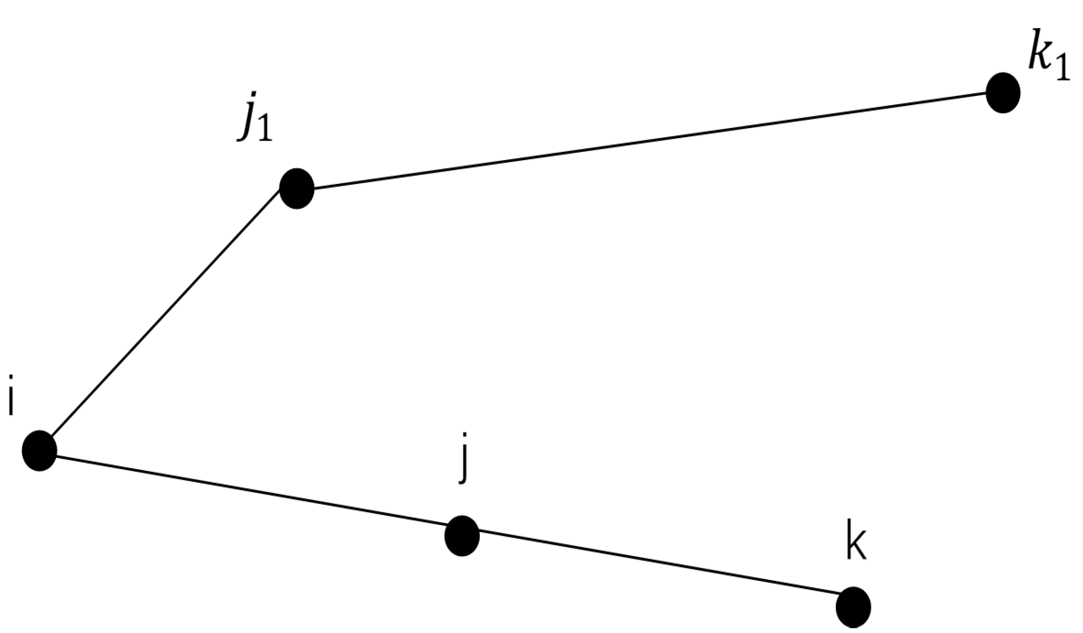
and the price of resources. From a global perspective, for the path with low scheduling cost, the local shortest path length does not mean it is the optimal result. In Figure 3, assume that

l_{i j_{1}} < l_{i j}

and

l_{j k} < l_{j_{1} k_{1}}

, but

l_{i k} < l_{i k_{1}}

, it can be concluded that the scheduling cost of each subpath is not necessarily the minimum on the path with the lowest scheduling cost.

For the large-scale distributed resource migration problem in this paper, the traditional ACO is likely to find a result with the lowest cost of layout migration in the first iteration, thus missing the set of migration nodes with the lowest total scheduling cost. In order to solve this problem, in the first iteration, the product of the distance between nodes and the number of ant colonies is used to quotient with the node size in the same cell to avoid local nodes with greedy ideas selected in the first iteration, which leads to global failure to find the optimal solution and rapid fall into the optimal local solution. Therefore, the formula of pheromone initialization distribution in our improved ACO is:

τ_{i j} (0) = \{\begin{matrix} \frac{d_{i j} \times m}{n} & i \neq j \\ 0 & i = j \end{matrix}

(10)

4.2. Parameter optimization of the ACO based on PSO

Because the ACO has many parameters, the setting of parameters directly impacts the optimization results. However, manually set parameter values cannot guarantee the optimization effect; therefore, how to reasonably set the parameters of the ACO before each iteration is the key to determining the algorithm’s performance. This paper proposes a parameter optimization method based on the PSO, which can dynamically optimize parameters according to the results of each iteration.

The PSO is a phenomenon that simulates birds searching for food. PSO has been widely used in continuous optimization problems and discrete optimization problems[32,33,34]. A population of m particles has its position in the multidimensional search space. The particles fly at a certain speed to simulate the migration process of birds. When searching for the target, focus on the best solution in this history search record and update the speed and position according to specific rules based on the best record of other particle history searches in this group.

The position of the d-th

(1 \leq d \leq m)

particle in the i-th particle group is expressed as

x_{i d}

, whose speed is expressed as

v_{i d}

, and whose best history is expressed as

p_{i d}

. The best record of all particles in the population is expressed as

p_{g d}

. The update of particle speed and position is based on the following two formulas:

\begin{matrix} v_{i d} & = & ω \times v_{i d} + c_{1} \times rand () \times (p_{i d} - x_{i d}) \\ + c_{2} \times rand () \times (p_{g d} - x_{i d}) \end{matrix}

(11)

x_{i d} = x_{i d} + v_{i d}

(12)

Where

ω

is the inertia weight, whose value determines how much of the past value of the particle remains. Whether

ω

is appropriate can determine whether the final solution is enough for optimization.

c_{1}

and

c_{2}

are called learning factors, equivalent to measuring the speed of particles approaching the optimal solution. The learning factor has the effect of evaluating itself and learning other particles. rand() is a pseudorandom number in the interval

[0, 1]

In this paper, the parameters

α

β

of the traditional ACO are optimized by training. Moreover, a mutation strategy is set so that when the ant selects a new node, the probability of selecting the next hop node through the pheromone concentration is no longer an inevitable event but has a certain probability of modifying the probability of selection.

In this algorithm, the total number of

N_{a}

ants is divided into several populations, and the number of ants in each population is the same

N_{s a}

. Each population maintains its pheromone matrix, which records the path between each node and the migration cost. Then convert position x and speed v into parameters

{α, β}

; The PSO is used to optimize these two parameters after each iteration of the ant colony algorithm as the initial parameters of the next iteration. The value range of

α

is set to

[1, 2]

, and the value range of

β

is set to

[1, 2]

. So the lower bound of

{α, β}

{1, 1}

, and

σ

is the difference between the upper and lower bound. Set the range of particle position to

[- 50, 50]

and particle speed to

[- 60, 60]

Suppose

X_{k}

is the

k - t h

position element of the particle; then, the particle position is converted into a parameter by the following formula.

\{α, β\} = R_{m i n} + σ * \frac{X_{k} - X_{m i n}}{X_{m a x} - X_{m i n}}

(13)

The traditional PSO is improved, and optimized

ω

to make it dynamic.

\begin{matrix} v_{i d} & = & ω^{(t)} \times v_{i d} + c_{1} \times rand () \times (p_{i d} - x_{i d}) \\ + c_{2} \times rand () \times (p_{g d} - x_{i d}) \end{matrix}

(14)

where

ω^{(t)} = \frac{(ω_{i n i} - ω_{e n d}) (G_{k} - g)}{G_{k} + ω_{e n d}}

Parameter

G_{k}

is the maximum number of iterations,

ω_{i n i}

is the initial inertia weight, and

ω_{e n d}

is the inertial weight value when the number of iterations reaches the maximum. Dynamic

ω

can achieve better results than fixed values and has more search options. Moving in a specific direction in parameter updating is not easy, but it has more significant opportunities to search unknown fields.

4.3. Improvement of selection probability

To solve the problem that the ACO can easily fall into the local optimum and converge to a local solution quickly, we propose the idea of selective mutation. Set a Variation Index (VI). Random variation will occur when the probability of selecting the next node is more significant than VI. She mutates the selection probability, which is half of the original probability, and the selection probability of other nodes should also be changed accordingly. The probability formula for selecting the next node is:

p_{i j - n e w}^{k} (t) = \{\begin{matrix} p_{i j}^{k} (t) \times \frac{1}{1 + \frac{δ}{t}} & p_{i j}^{k} (t) > VI \\ p_{i j}^{k} (t) & otherwise \end{matrix}

(15)

Where,

p_{i j}^{k} (t)

refers to the probability of selecting the next node, while

p_{i j - n e w}^{k} (t)

refers to the probability of selecting the next node after selection and variation.

δ

indicates the probability decay rate of the next node. t represents the current number of iterations. After selecting one node changes, the probability of selecting other nodes will be normalized accordingly; that is, the probability distribution of the final roulette selection can be obtained.

According to the formula14, when the value of t is minimal, that is, in the first few iterations, the value of

p_{i j}^{k} (t)

has a significant attenuation. With the increasing value of t, the probability of selecting the next node will be closer to the original unchanged probability. The advantage of this is that when the number of iterations is small, it can better weaken the probability of selecting the next node so that the algorithm has better breadth and randomness when searching for nodes and avoid quickly entering the optimal local value. With the increase in the number of iterations, the probability of modifying the selection of the next node becomes smaller and smaller and converges faster. It can ensure the breadth of ants searching for nodes and accelerate the speed of searching for the global approximate optimal solution.

This approach is not entirely blind and random to find new results, which cannot be called a random search. Because this selection mutation operation only weakens the probability that the path with too much influence is selected, rather than discarding this probability, it makes up the defect that the algorithm converges to the optimal local solution too quickly.

4.4. Pheromone updating and improvement

The improvement of pheromone updating rules and pheromone incremental updating rules interact. The traditional ACO for pheromone incremental updating rules converges too slowly. The reason is that the pheromone updating is too slow, which makes the algorithm unable to converge to the path at a low cost quickly. After analyzing the original pheromone incremental update formula(8), even though the cost of different nodes on the path is very different, the pheromone increment calculated by the formula is not significantly different. It is meaningless to choose a better path and cannot change the final selection strategy. Therefore, some improvements have been made to formula(8) to increase the difference of pheromone increments on the path with significant cost difference so that it has a more vital ability to select multiple paths. The improved formula is as follows:

\begin{matrix} Δ τ_{i j}^{k} = \{\begin{matrix} \frac{Q}{e^{L_{k} - A v g}} & if edge (i, j) in its tour \\ 0 & otherwise \end{matrix} \end{matrix}

(16)

Where Q is constant,

L_{k}

is the length of the current path;

A v g

is the average cost of all ants’ paths in this round. When the cost of an ant’s path is small, the concentration of the pheromone update is greater than that of Q. Furthermore, when the cost of an ant’s path is high, the concentration of the pheromone update is much smaller than that of Q, which can highlight the difference in the pheromone update value and increase the convergence speed of the algorithm. We have improved the pheromone updating rule to prevent the algorithm’s convergence rate from exceeding expectations.

τ_{i j} (t + n) = (1 - ρ) \times τ_{i j} (t) + ρ \times Δ τ_{i j}

(17)

See in algorithm 1, the heuristic algorithm flow designed in this paper is as follows:

Algorithm 1:Adaptive dynamic migration algorithm for large-scale distributed resources

1.35

Require:: Large-scale distributed network P
Ensure:: Resource scheduling optimization scheme R
1:: Initialize Parameters of particle swarm $v_{i d}$ , $x_{i d}$ , $t a b u_{k}$ , $N_{s a}$
2:: $\{α, β\} < - v_{i d}, x_{i d}$
3:: for k <- 1 to $N_{s a}$ do
4:: for i in P do
5:: ant k choose next park
6:: modify taboo list $t a b u_{k}$ of ant k
7:: if L $(i)$ < L $(k n o w n - b e s t)$ then
8:: replace best route
9:: L $(b e s t)$ <- L $(i)$
10:: Shortest route <- ${L (i)}_{r o u t e}$
11:: end if
12:: activity of pheromone updating is excuted
13:: activity of $v_{i d}$ , $x_{i d}$ updating is excuted
14:: end for
15:: R updating is excuted
16:: end for
17:: Return R

Initialize the parameters, randomly generate the parameters of the particle swarm (including the speed and position of each particle), and convert the parameters into $\{α, β\}$ .
Initialize the pheromone and other parameters of the ACO; Set $N_{s a}$ ants of each ant population on these nodes.
Make all ants in each ant population search for all nodes according to the formula(14). Select the target node to apply for resources, modify the scheduling table and calculate the total cost of scheduling resources.
Calculate the total scheduling cost of each population scheduling resource, and record the ant path corresponding to the optimal scheduling cost. The optimal scheduling generation value is used as the fitness value of the particle. The particle with the optimal fitness value selected is the best record of the current iteration number of the population. Update the best record of each particle’s history and the best record of the population’s history. After updating the speed and position according to formula(13), convert the position parameters to new ${α, β}$ according to formula(12). Update the value of pheromone according to formula(16).
If the number of iterations has reached the target number of iterations, stop the iteration; if the number of iterations does not meet the requirements, re-execute step(3).

5. Experimental analysis

According to the characteristics of the global resource scheduling problem of distributed edge computing, some data must be preprocessed on the dataset, which can better reflect the characteristics and structure of the model. We built a dataset including 50 nodes in different locations. To verify the performance of this algorithm, the greedy algorithm[35], the basic ACO[36], the GA[37], the Hybrid ACO-GA Algorithm (H3AGA)[38]. The Selective Mutation ACO (SMACA) in this paper is compared to the data set.

The current operations on this dataset include two aspects:

Accuracy comparison

To verify the algorithm’s accuracy proposed in this paper, we compare the objective function values of the scheduling results of different algorithms. If the objective function value is more significant after the scheduling is completed, this algorithm’s scheduling results are closer to the optimal solution.
Iteration cost comparison

The iteration cost of the algorithm is the number of iterations, which is also a critical performance index. We set the iteration times of different algorithms under the same target conditions.

Table 1 shows the algorithm parameter setting information of this experiment.

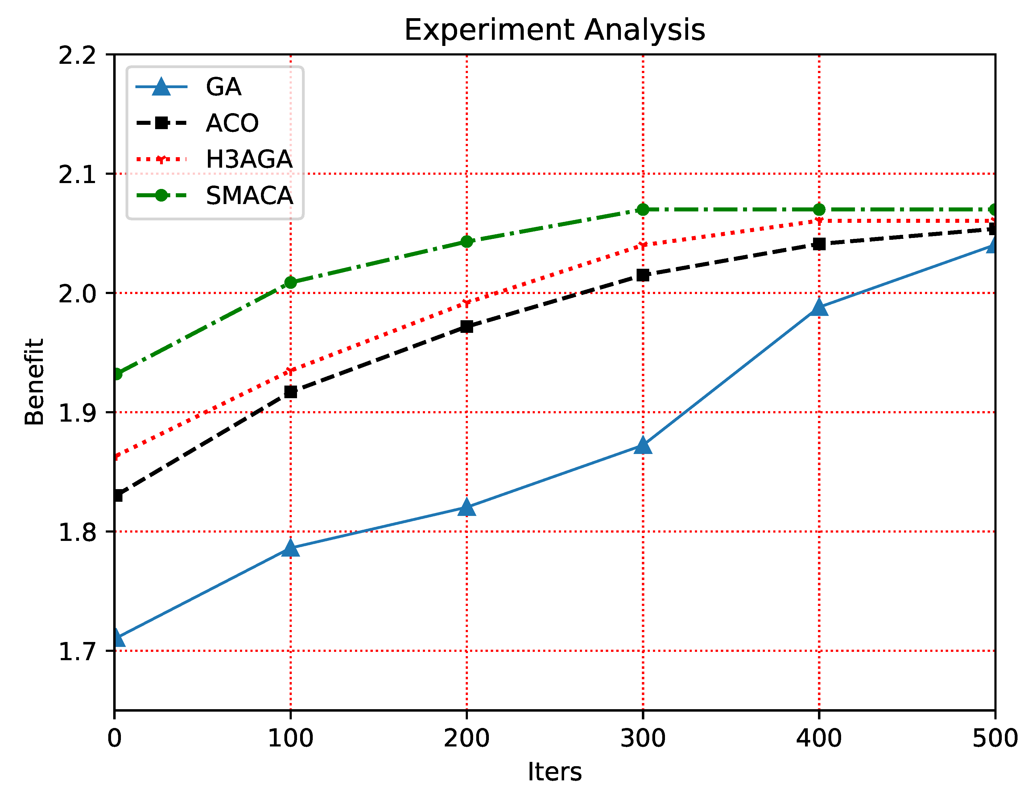
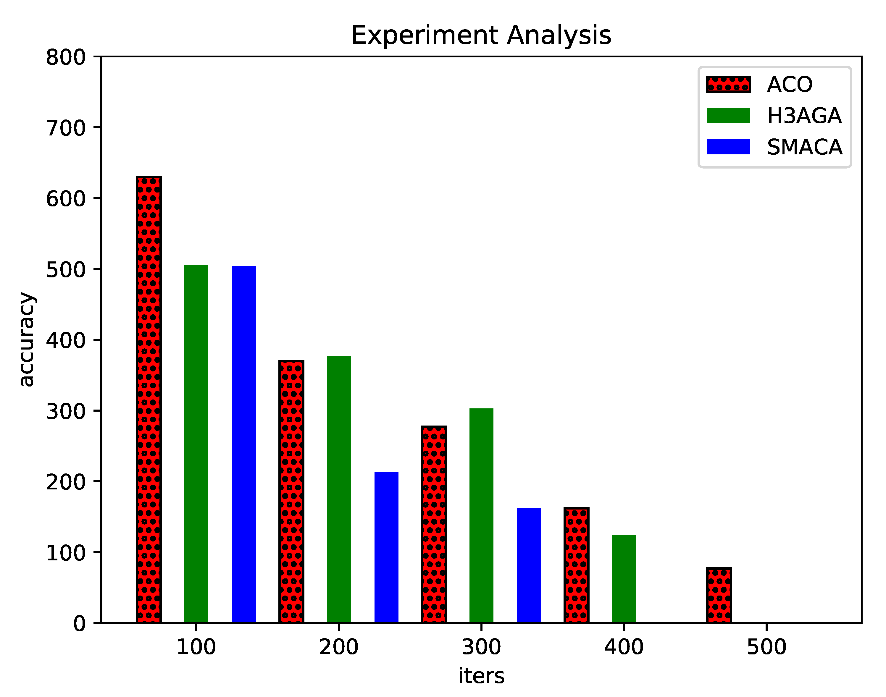
We judge the algorithm’s accuracy by the objective function value. If the value of the objective function is greater, the algorithm’s accuracy is better under the same iteration number. Figure 4 shows the experimental results of algorithm accuracy. The abscissa represents the iteration number of the algorithm, and the ordinate represents the objective function value of different algorithms under the same iteration number. In the first few iterations, the accuracy of the GA is significantly lower than the other three algorithms. However, with the gradual increase in the number of iterations, the accuracy of the GA is improving. Compared with the three different algorithms, the convergence speed of the SMACA proposed in this paper is significantly better than the ACO and H3AGA. It can approach the maximum target value at the fastest speed. With the increase in the number of iterations, the value of the objective function of the ACO has been increasing, and the convergence time is the longest among several ant colony algorithms. The H3AGA converged before the 400th iteration, while the number of iterations required for the SMACA to converge is about 200-300. In general, the SMACA can significantly reduce iteration time cost, has the fastest convergence, and has a significant advantage in accuracy. This experimental result is because SMACA dynamically adjusts when selecting the next node and balances the convergence rate when updating the pheromone. The result of the greedy algorithm does not depend on multiple iterations, so it cannot be compared with other heuristic algorithms in terms of convergence speed and accuracy.

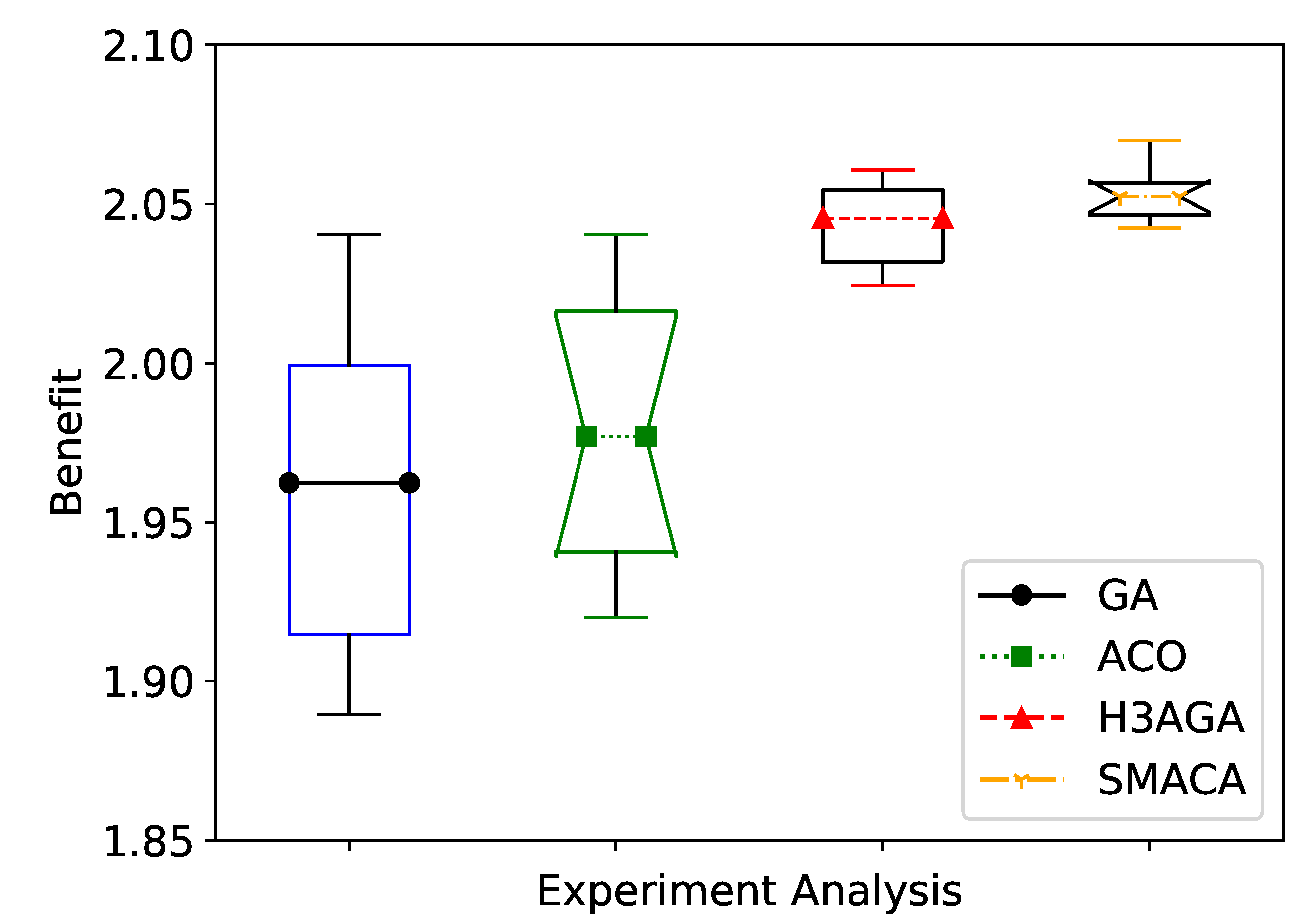
Because the results of a single experiment may need to be more accurate due to randomness, this paper will repeat each experiment 20 times. The results of 20 experiments will be displayed in a boxplot, as shown in Figure 5. The abscissa in the figure represents different algorithms, and the ordinate represents the objective function value. In the statistics of large samples, the experimental results of the GA are very dependent on the randomness of mutation and the population size. The experimental results of the ACO and H3AGA are evenly distributed. Compared with other algorithms, the experimental results of SMACA are more concentrated and less random. Therefore, the algorithm proposed in this paper has excellent stability.

In finding the minimum scheduling cost, the standard to measure the merits of an algorithm is whether it can be closer to the actual minimum value. Due to the large scale of the problem and other reasons, we can not get the real minimum value. Therefore, a new concept is introduced here: precision. The precision is defined here as the difference between the minimum value obtained by the algorithm and the smaller minimum value obtained by the next iteration. The smaller the difference, the closer it is to the minimum value. In this way, we can conclude that when various algorithms get the same accuracy, which algorithm needs more iterations and which is closer to the actual minimum? Applying this conclusion to this problem, we can transform it to obtain the following criteria. When the iteration times of various algorithms are the same, the smaller the accuracy is, the better the algorithm is.

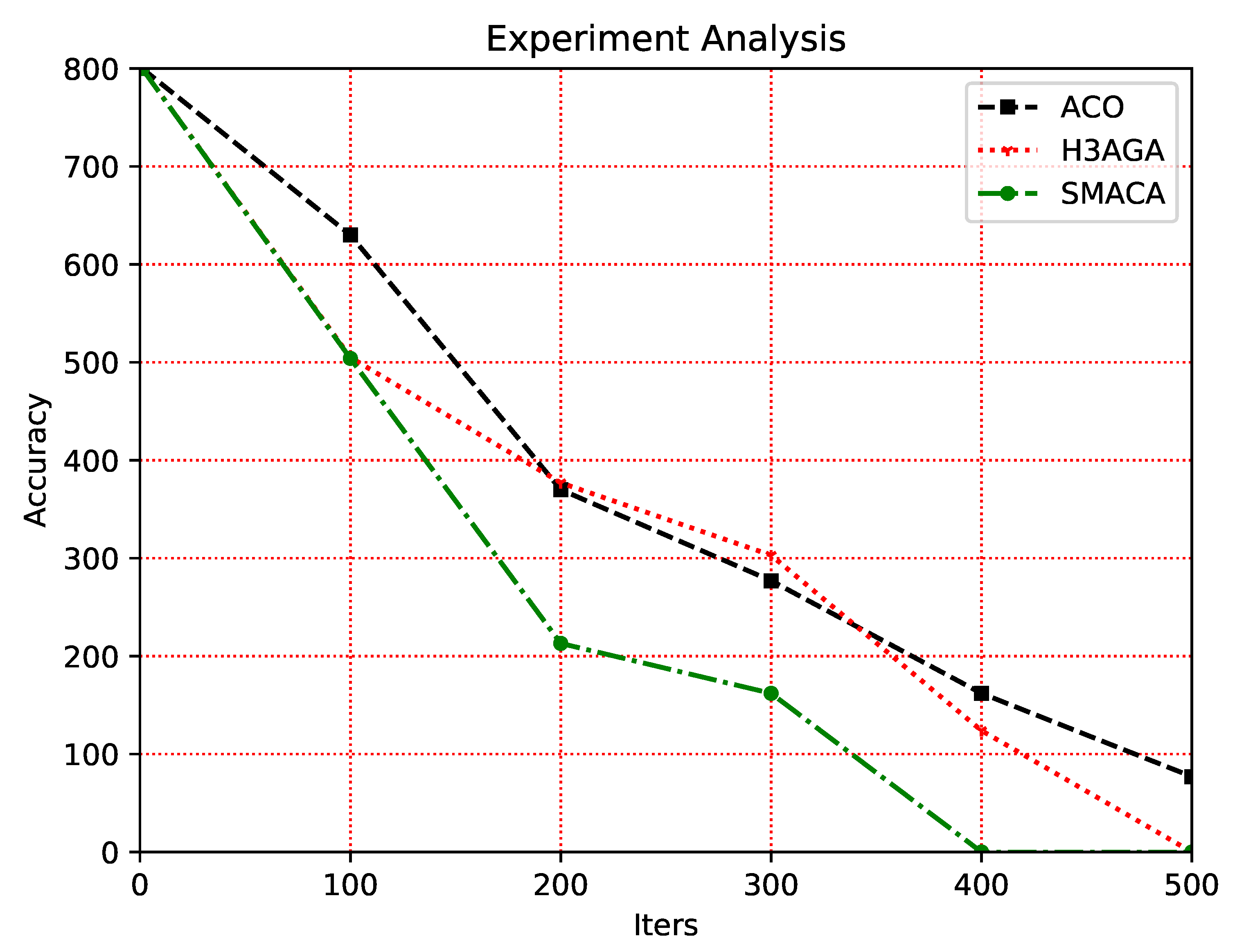
Due to the characteristics of the GA, its results have great uncertainty, so a precision comparison cannot be made. This paper compares the accuracy of the other three algorithms. Figure 6 and Figure 7 show the actual effect comparison of each algorithm in two different forms. The abscissa represents the number of iterations, and the ordinate represents the precision value of the algorithm. With the increase in the number of iterations, the accuracy value of each algorithm has improved. The accuracy of the SMACA is always better than the ACO and H3AGA. It can reduce its accuracy value to 0 with fewer iterations, which shows that the SMACA has a better convergence speed.

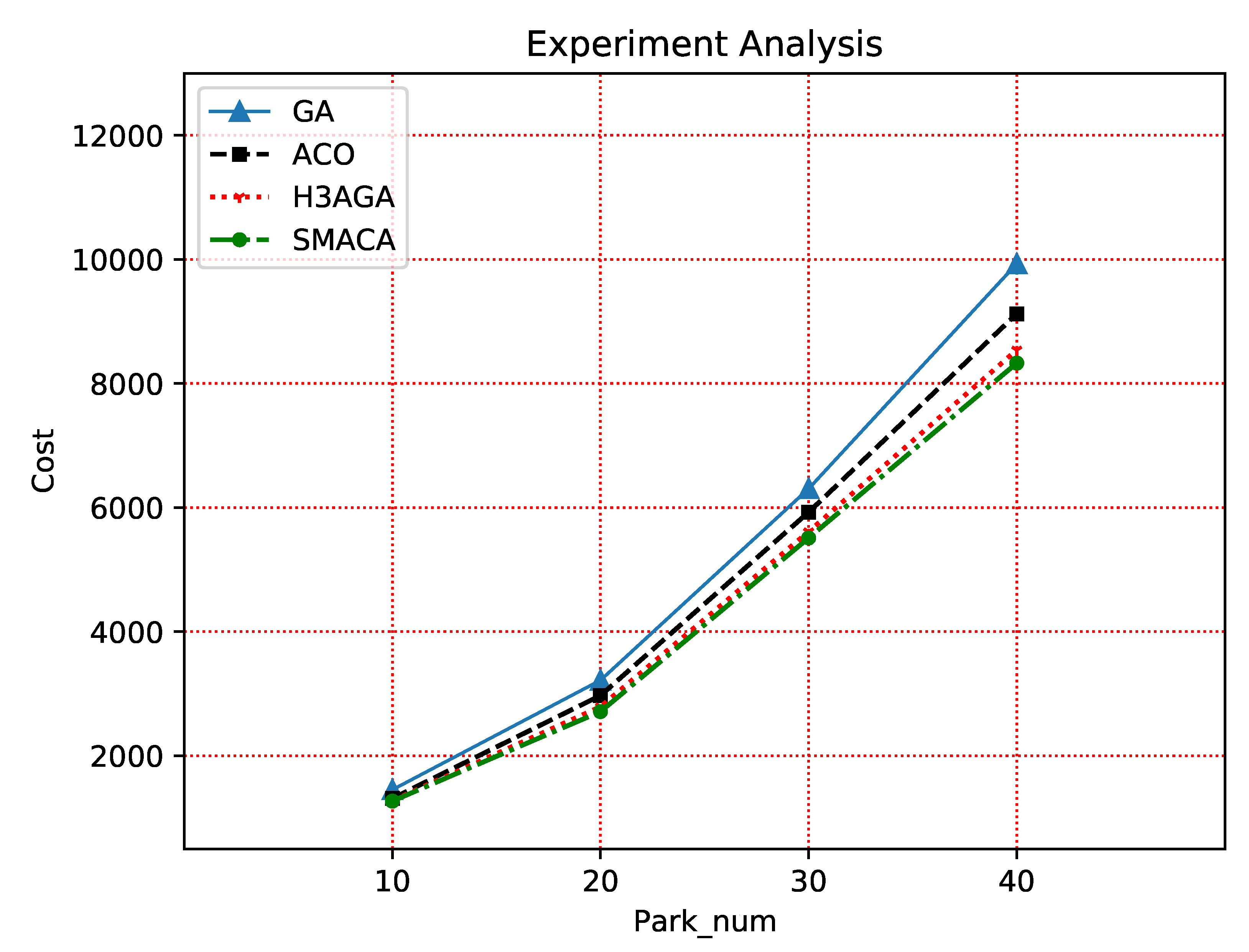
The number of nodes is an essential factor determining the algorithm’s performance. This paper designs a comparative experiment of the algorithm performance under different node numbers. In Figure 8, the abscissa represents the number of parks (each park contains multiple nodes), and the ordinate represents the migration cost. As the number of nodes increases, the cost of resource migration will increase. It is because after the number of nodes increases, the resource scheduling of any node will be determined according to the objective function and constraint conditions, not only considering the nodes that are close to each other, so this increase in cost is inevitable. Compared with other algorithms, the SMACA in this paper performs better regarding average migration cost.

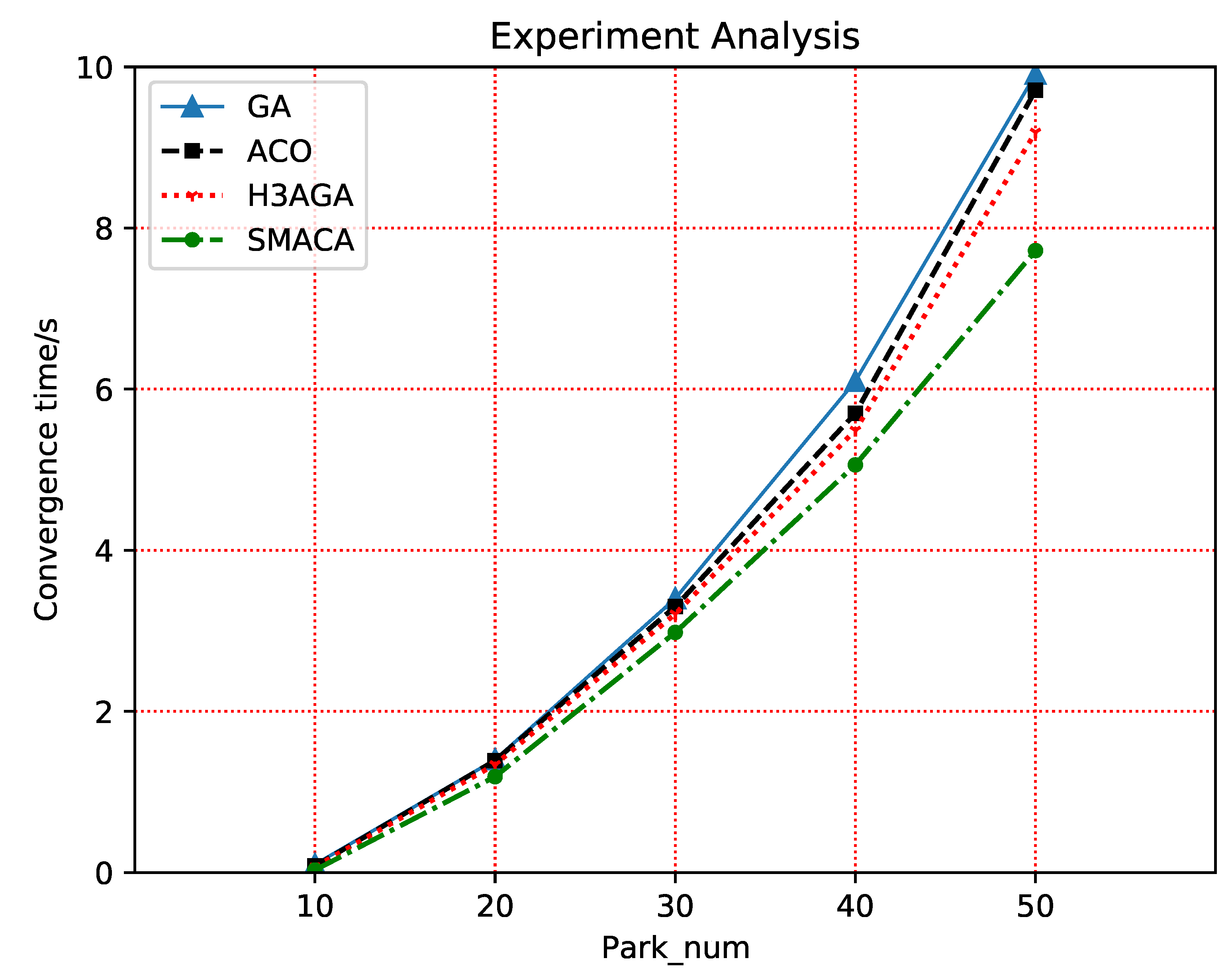
It can be seen from the changing trend of the interval distance of each curve in Figure 9 that the convergence time of the four algorithms is the same when the node size is small. With the increasing number of nodes, the SMACA’s advantages are more apparent and more suitable for large-scale datasets. The reason for this is the improvement of pheromone updating rules, which significantly expands the difference of pheromone updating amount on paths with different costs, makes it easier to choose the path with low cost, and greatly optimizes the convergence speed of the algorithm.

According to the above experimental results, the SMACA can perform better on the adaptive migration of large-scale distributed resources.

6. Conclusion

This paper studies the application of adaptive dynamic migration of large-scale distributed resources and the defects and deficiencies of current research. It gives mathematical modeling and a formulaic definition of this problem. The computational complexity of the defined problem is analyzed, and it is proved that the problem is NP-Hard. The heuristic algorithm is designed based on ACO, and the parameters of the ACO are intelligently adjusted through PSO. This algorithm absorbs the advantages of the PSO and ACO. Finally, the comparative experimental analysis of several algorithms shows that the algorithm designed in this paper has good performance for large-scale distributed resource migration.

This paper focuses on the mathematical model design and computational complexity analysis of complex engineering problems. At the algorithm level, this paper uses the relatively basic PSO to update the parameters of the ACO. It improves each step of the ACO to solve the large-scale distributed resource scheduling problem. However, the ACO cannot guarantee the optimal solution. Therefore, the follow-up work will explore how to design the algorithm to solve the optimal solution.

Acknowledgments

This work is supported in part by National Key R&D Program of China (2019YFB1406002).

References

Stray, V.; Moe, N.B.; Vedal, H.; Berntzen, M. Using objectives and key results (OKRs) and slack: a case study of coordination in large-scale distributed agile 2021. [CrossRef]
Kang, P.; Deng, H.; Wang, X. Research on Multi-Equipment Collaborative Scheduling Algorithm under Composite Constraints. Processes 2022, 10, 1171. [CrossRef]
Deshmukh, S.; Thirupathi Rao, K.; Shabaz, M. Collaborative learning based straggler prevention in large-scale distributed computing framework. Security and communication networks 2021, 2021. [CrossRef]
Jia, Y.H.; Chen, W.N.; Gu, T.; Zhang, H.; Yuan, H.Q.; Kwong, S.; Zhang, J. Distributed cooperative co-evolution with adaptive computing resource allocation for large scale optimization. IEEE Transactions on Evolutionary Computation 2018, 23, 188–202. [CrossRef]
Askarizade Haghighi, M.; Maeen, M.; Haghparast, M. An energy-efficient dynamic resource management approach based on clustering and meta-heuristic algorithms in cloud computing IaaS platforms. Wireless Personal Communications 2019, 104, 1367–1391. [CrossRef]
Yuan, M.; Li, Y.; Zhang, L.; Pei, F. Research on intelligent workshop resource scheduling method based on improved NSGA-II algorithm. Robotics and Computer-Integrated Manufacturing 2021, 71, 102141. [CrossRef]
Zhang, R.; Shi, W. Research on workflow task scheduling strategy in edge computer environment. In Proceedings of the Journal of Physics: Conference Series. IOP Publishing, 2021, Vol. 1744, p. 032215. [CrossRef]
Rjoub, G.; Bentahar, J.; Abdel Wahab, O.; Saleh Bataineh, A. Deep and reinforcement learning for automated task scheduling in large-scale cloud computing systems. Concurrency and Computation: Practice and Experience 2021, 33, e5919. [CrossRef]
Li, B.; Pang, R.; Sainath, T.N.; Gulati, A.; Zhang, Y.; Qin, J.; Haghani, P.; Huang, W.R.; Ma, M.; Bai, J. Scaling end-to-end models for large-scale multilingual ASR. In Proceedings of the 2021 IEEE Automatic Speech Recognition and Understanding Workshop (ASRU). IEEE, 2021, pp. 1011–1018.
Muhtadi, A.; Pandit, D.; Nguyen, N.; Mitra, J. Distributed energy resources based microgrid: Review of architecture, control, and reliability. IEEE Transactions on Industry Applications 2021, 57, 2223–2235. [CrossRef]
Liu, S.; Hennequin, S.; Roy, D. Enterprise Platform of Logistics Services Based on a Multi-Agents Mechanism and Blockchains. IFAC-PapersOnLine 2021, 54, 825–830. [CrossRef]
Sheng, J.; Hu, Y.; Zhou, W.; Zhu, L.; Jin, B.; Wang, J.; Wang, X. Learning to schedule multi-NUMA virtual machines via reinforcement learning. Pattern Recognition 2022, 121, 108254. [CrossRef]
Guo, D.; Olesen, J.E.; Manevski, K.; Ma, X. Optimizing irrigation schedule in a large agricultural region under different hydrologic scenarios. Agricultural Water Management 2021, 245, 106575.
Cui, L.; Liu, X.; Lu, S.; Jia, Z. A variable neighborhood search approach for the resource-constrained multi-project collaborative scheduling problem. Applied Soft Computing 2021, 107, 107480. [CrossRef]
Wu, Y.; Sun, X. Optimization and simulation of enterprise management resource scheduling based on the radial basis function (RBF) neural network. Computational Intelligence and Neuroscience 2021, 2021. [CrossRef]
Yuan, M.; Cai, X.; Zhou, Z.; Sun, C.; Gu, W.; Huang, J. Dynamic service resources scheduling method in cloud manufacturing environment. International Journal of Production Research 2021, 59, 542–559. [CrossRef]
Wang, Z.J.; Zhan, Z.H.; Yu, W.J.; Lin, Y.; Zhang, J.; Gu, T.L.; Zhang, J. Dynamic group learning distributed particle swarm optimization for large-scale optimization and its application in cloud workflow scheduling. IEEE transactions on cybernetics 2019, 50, 2715–2729. [CrossRef]
Jiang, F.; Dong, L.; Wang, K.; Yang, K.; Pan, C. Distributed resource scheduling for large-scale MEC systems: A multiagent ensemble deep reinforcement learning with imitation acceleration. IEEE Internet of Things Journal 2021, 9, 6597–6610. [CrossRef]
Envelope, M.; Envelope, M.; Envelope, M. Task offloading using GPU-based particle swarm optimization for high-performance vehicular edge computing. Journal of King Saud University - Computer and Information Sciences 2022. [CrossRef]
Zhang, X.; Du, K.J.; Zhan, Z.H.; Kwong, S.; Zhang, J. Cooperative Coevolutionary Bare-Bones Particle Swarm Optimization With Function Independent Decomposition for Large-Scale Supply Chain Network Design With Uncertainties. IEEE Transactions on Cybernetics 2019, PP, 1–15. [CrossRef]
Sajid, M.; Mittal, H.; Pare, S.; Prasad, M. Routing and scheduling optimization for UAV assisted delivery system: A hybrid approach. Applied Soft Computing 2022, 126, 109225. [CrossRef]
Jahic, A.; Plenz, M.; Eskander, M.; Schulz, D. Route scheduling for centralized electric bus depots. IEEE Open Journal of Intelligent Transportation Systems 2021, 2, 149–159. [CrossRef]
Li, H.; Wu, X.; Kou, K.P.; et al. Near-optimal fixed-route scheduling for crowdsourced transit system. In Proceedings of the 2021 IEEE 37th International Conference on Data Engineering (ICDE). IEEE, 2021, pp. 2273–2278.
Mousa, M.H.; Hussein, M.K. Effcient UAV-Based MEC Using GPU-Based PSO and Voronoi Diagrams. Computer Modeling in Engineering and Sciences 2022, p. 000. [CrossRef]
Agiwal, M.; Kwon, H.; Park, S.; Jin, H. A survey on 4G-5G dual connectivity: road to 5G implementation. IEEE Access 2021, 9, 16193–16210. [CrossRef]
Son, J.; Buyya, R. Latency-aware virtualized network function provisioning for distributed edge clouds. Journal of Systems and Software 2019, 152, 24–31. [CrossRef]
Zhao, Z.; Barijough, K.M.; Gerstlauer, A. Deepthings: Distributed adaptive deep learning inference on resource-constrained iot edge clusters. IEEE Transactions on Computer-Aided Design of Integrated Circuits and Systems 2018, 37, 2348–2359. [CrossRef]
Hu, J.; Liu, X.; Shahidehpour, M.; Xia, S. Optimal operation of energy hubs with large-scale distributed energy resources for distribution network congestion management. IEEE Transactions on Sustainable Energy 2021, 12, 1755–1765. [CrossRef]
Zhang, Y.; Wu, J.; Liu, M.; Tan, A. TSN-based routing and scheduling scheme for Industrial Internet of Things in underground mining. Engineering Applications of Artificial Intelligence 2022, 115, 105314. [CrossRef]
Peng, Y.; Ning, Z.; Tan, A.; Wang, S.; Obaidat, M.S. A Delay-Sensitive Multibase-Station Multichannel Access System for Smart Factory. IEEE Systems Journal 2022. [CrossRef]
Hartmanis, J. Computers and intractability: a guide to the theory of np-completeness (michael r. garey and david s. johnson). Siam Review 1982, 24, 90.
Jian, J.R.; Chen, Z.G.; Zhan, Z.H.; Zhang, J. Region Encoding Helps Evolutionary Computation Evolve Faster: A New Solution Encoding Scheme in Particle Swarm for Large-Scale Optimization. IEEE Transactions on Evolutionary Computation 2021, PP, 1–1. [CrossRef]
Xia, X.; Gui, L.; Yu, F.; Wu, H.; Zhan, Z.H. Triple Archives Particle Swarm Optimization. IEEE Transactions on Cybernetics 2019, PP, 1–14. [CrossRef]
Li, J.Y.; Zhan, Z.H.; Liu, R.D.; Wang, C.; Zhang, J. Generation-Level Parallelism for Evolutionary Computation: A Pipeline-Based Parallel Particle Swarm Optimization. IEEE Transactions on Cybernetics 2020, PP, 1–12. [CrossRef]
Edmonds, J. Matroids and the greedy algorithm. Mathematical programming 1971, 1, 127–136.
Dorigo, M.; Birattari, M.; Stutzle, T. Ant colony optimization. IEEE computational intelligence magazine 2006, 1, 28–39.
Whitley, D. A genetic algorithm tutorial. Statistics and computing 1994, 4, 65–85. [CrossRef]
Liu, J.; Xu, S.; Zhang, F.; Wang, L. A hybrid genetic-ant colony optimization algorithm for the optimal path selection. Intelligent Automation & Soft Computing 2017, 23, 235–242. [CrossRef]

Figure 1. The case of large-scale distributed resource migration and scheduling

Figure 2. Topology of the problem

Figure 3. Example of path selection for global optimization and local optimization

Figure 4. Comparison of algorithm minimum cost

Figure 5. Distribution of multiple experimental results of different algorithms

Figure 6. Accuracy comparison plot of different algorithms

Figure 7. Accuracy comparison histogram of different algorithms

Figure 8. Cost comparison of different algorithm scales

Figure 9. Comparison of convergence time of different algorithms based on scale

Table 1. The parameter setting of the experiment

Id	Algorithm	Parameter
1	ACO	$τ = 1$ , $ρ = 0.2$ , $α = 1$ , $β = 2$ , $m = 50$ , $T = 1000$
2	GA	The crossing probability value is set as 0.75, the variation probability is 0.05, the population size is 1000, and the chromosome length is 50.

Disclaimer/Publisher’s Note: The statements, opinions and data contained in all publications are solely those of the individual author(s) and contributor(s) and not of MDPI and/or the editor(s). MDPI and/or the editor(s) disclaim responsibility for any injury to people or property resulting from any ideas, methods, instructions or products referred to in the content.

© 2023 by the authors. Licensee MDPI, Basel, Switzerland. This article is an open access article distributed under the terms and conditions of the Creative Commons Attribution (CC BY) license (http://creativecommons.org/licenses/by/4.0/).

Copyright: This open access article is published under a Creative Commons CC BY 4.0 license, which permit the free download, distribution, and reuse, provided that the author and preprint are cited in any reuse.

MDPI Initiatives

Important Links

Choose an area of interest and we will send you notifications of new preprints at your preferred frequency.

Disclaimer

A Global Resource Scheduling for Distributed Edge Computing

Abstract

1. Introduction

2. Related work

3. System formulation

3.1. Problem definition

3.2. Computational complexity analysis

4. Algorithm design

4.1. Design of heuristic algorithm based on ACO

4.2. Parameter optimization of the ACO based on PSO

4.3. Improvement of selection probability

4.4. Pheromone updating and improvement

5. Experimental analysis

6. Conclusion

Acknowledgments

References

MDPI Initiatives

Important Links

Subscribe