Submitted:
12 October 2023
Posted:
13 October 2023
You are already at the latest version
Abstract

Keywords:
1. Introduction
- The study compares the predictive performance of machine learning algorithms: k-nearest neighbors, Random Forest, Gradient Boosting Machines, and classical statistic models: logistic regression in glacier mapping. It is expected that the machine learning algorithms will demonstrate significantly higher predictive performance.
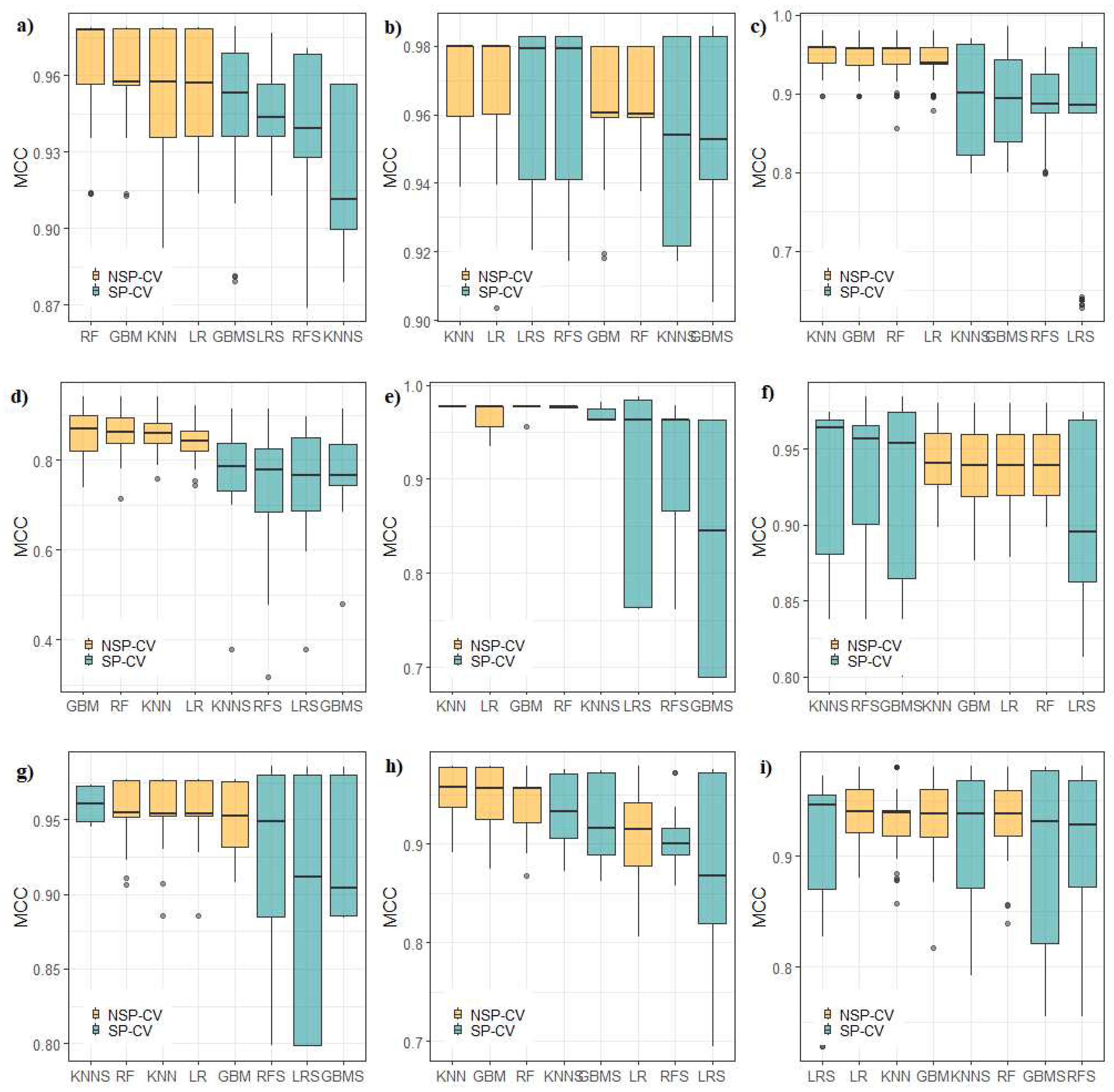
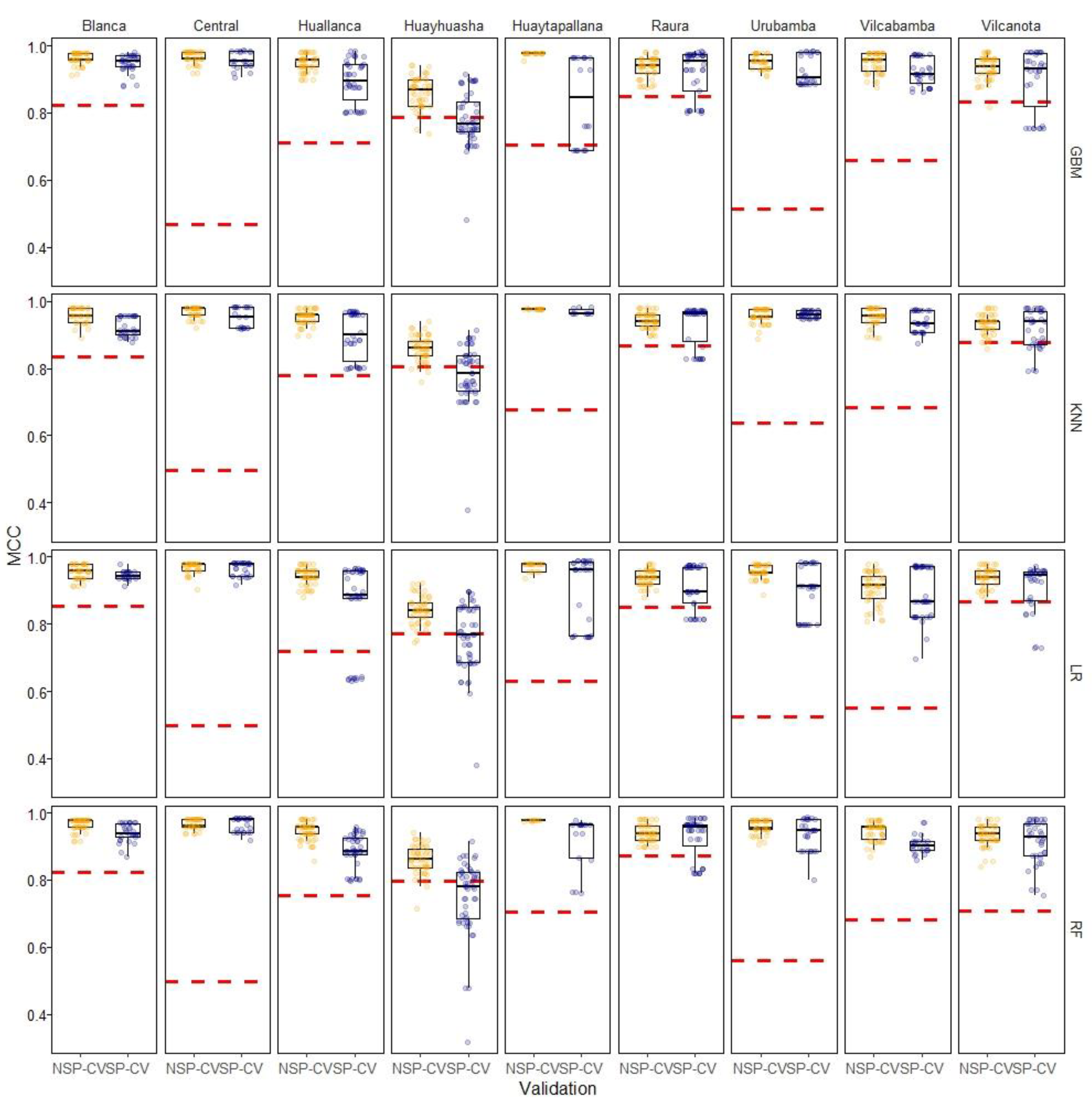
- The study also examines the predictive performance of classification algorithms when spatial and non-spatial cross-validation methods are used. It is hypothesized that non-spatial partitioning methods will yield over-optimistic results due to the presence of spatial autocorrelation.
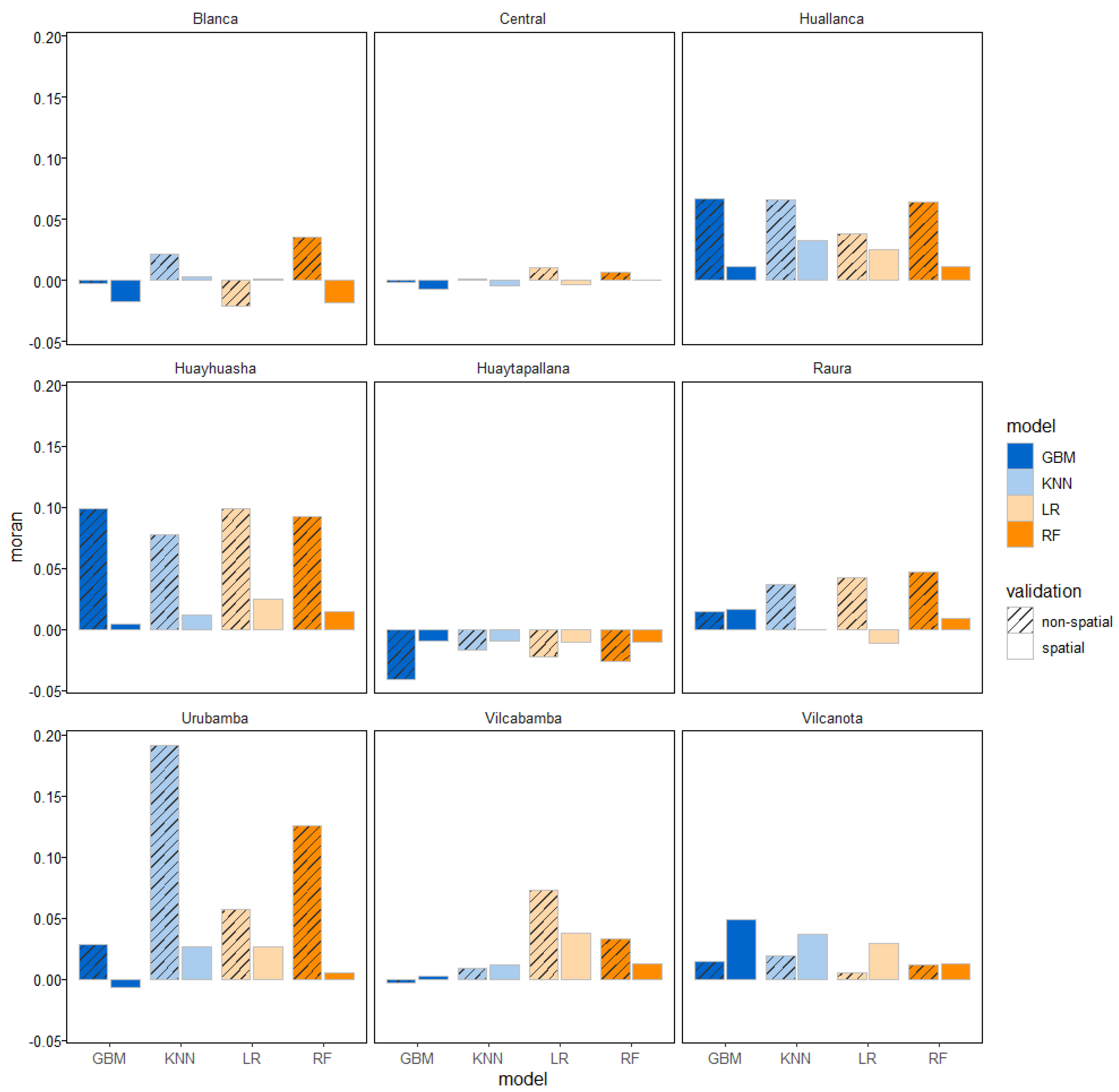
- Additionally, the study investigates the effects of spatial clustering on the distribution of errors in the analyzed algorithms for glacier mapping. It is anticipated that non-spatial models will exhibit spatial autocorrelation in their errors.
2. Materials and Methods
2.1. Study Area
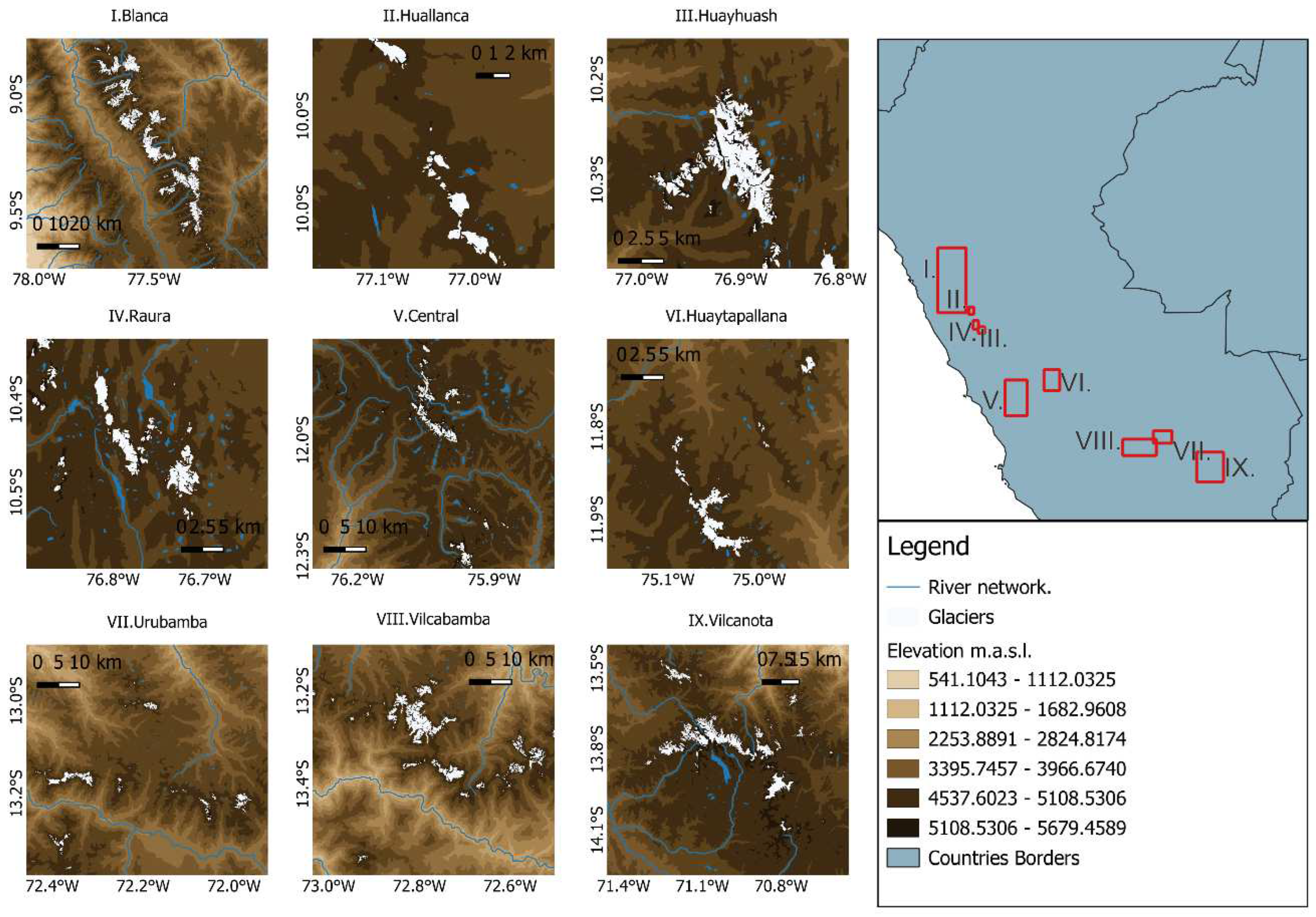
- R1 is the northern wet outer tropics, with a high mean annual humidity of 71 %, nearly no seasonality of the temperature and a total annual precipitation of 815 mm. R1 includes the Cordillera Blanca, Central, Chonta, Huagoruncho, Huallanca, Huayhuash, Huaytapallana, La viuda and Raura.
- R2 is the southern wet outer tropics, with moderate mean annual humidity of 59 %, an annual variability of the mean monthly temperature of about 4 ◦C and a total annual precipitation of 723 mm. R2 includes the Cordillera Vilcabamba, Urubamba, Vilcanota, Carabaya and Apolobamba.
- R3 is the dry outer tropics, with low mean annual humidity of 50 %, a mean annual temperature of −4.0 ◦C and low total annual precipitation of 287 mm. R3 includes the Cordillera Ampato and Coropuna.
2.2. Data Acquisition
2.2.1. Glacier Inventory
2.2.2. Landsat Data and Processing
2.2.3. Normalized Difference Snow Index (NDSI)
2.2.4. Digital Elevation Model (DEM)
2.2.5. Pixel Sampling and Classification Matrix Assembly
2.3. Machine Learning Classifiers
2.3.1. Logistic Regression
2.3.2. k-Nearest Neighbors
2.3.3. Random Forest
2.3.4. Gradient Boosting Machines
2.4. Implementation
2.5. Model Evaluation Metrics
2.5.1. Matthews Correlation Coefficient (MCC)
2.5.2. Moran’s I
2.5.3. Spatial Autocorrelation of Glacier Class
2.6. Spatial Vs. Non-Spatial CV Comparison Experiment
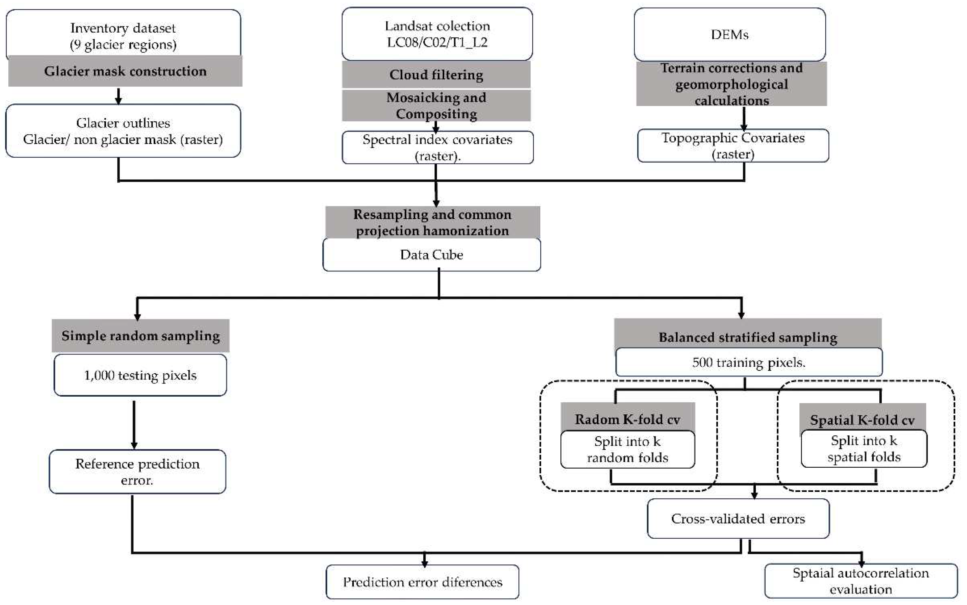
2.6.1. Step 1: Construction of Sample Data and Prediction Locations
2.6.2. Step 2: Calculate Reference Prediction Error
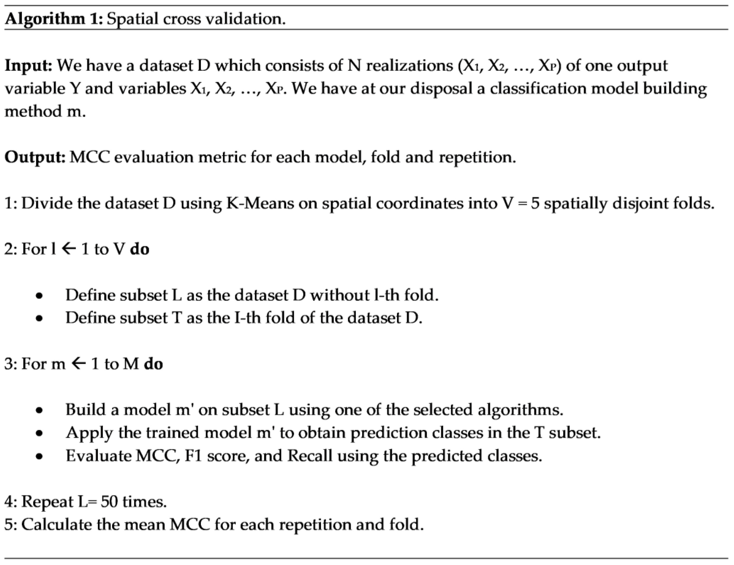
2.6.3. Step 3: Calculate the Prediction Error of Each CV Method
2.6.4. Step 4: Calculate CV Method’s Prediction Error Difference
2.7. Satistical Comparison of Model Results
3. Results and Discussion
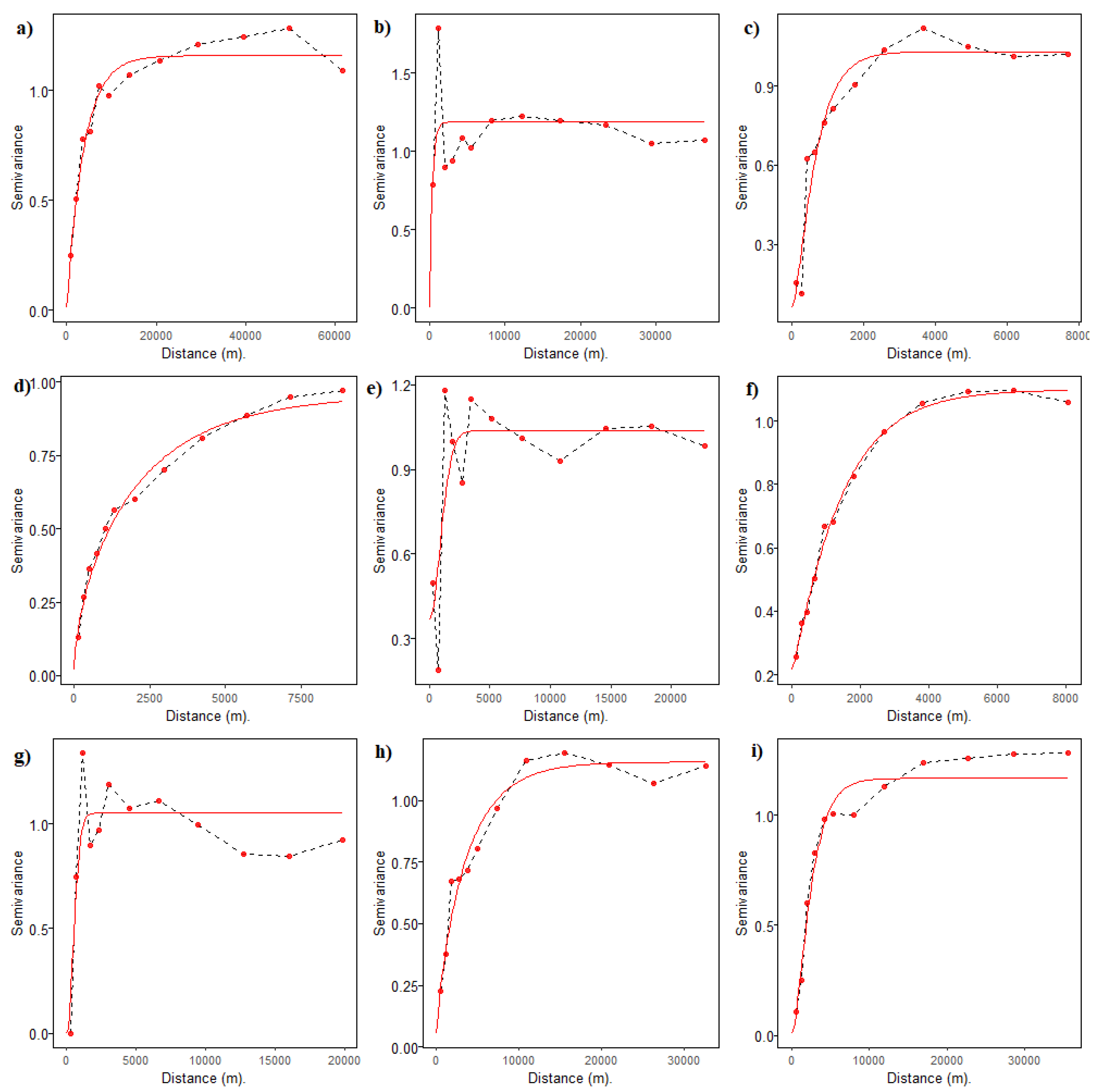
3.1. Spatial Autocorrelation
3.2. Model Specification
3.3. Spatial Vs. Non-Spatial CV Comparison Experiment
3.4. Satistical Comparison of Model Results
3.5. Spatial Autocorrelation of Errors
3.6. Spatial Predictions
3.7. Methodological Limitations of the Study
4. Conclusions
Author Contributions
Funding
Data Availability Statement
Acknowledgments
Conflicts of Interest
References
- Veettil, B.K.; Kamp, U. Remote Sensing of Glaciers in the Tropical Andes: A Review. International Journal of Remote Sensing 2017, 38, 7101–7137. [Google Scholar] [CrossRef]
- Drenkhan, F.; Carey, M.; Huggel, C.; Seidel, J.; Oré, M.T. The Changing Water Cycle: Climatic and Socioeconomic Drivers of Water-related Changes in the Andes of Peru. WIREs Water - Wiley Online.
- Salzmann, N.; Huggel, C.; Rohrer, M.; Silverio, W.; Mark, B.G.; Burns, P.; Portocarrero, C. Glacier Changes and Climate Trends Derived from Multiple Sources in the Data Scarce Cordillera Vilcanota Region, Southern Peruvian Andes. The Cryosphere 2013, 7, 103–118. [Google Scholar] [CrossRef]
- Taylor, L.S.; Quincey, D.J.; Smith, M.W.; Potter, E.R.; Castro, J.; Fyffe, C.L. Multi-Decadal Glacier Area and Mass Balance Change in the Southern Peruvian Andes. Frontiers in Earth Science 2022, 10. [Google Scholar] [CrossRef]
- Silverio, W.; Jaquet, J.-M. Glacial Cover Mapping (1987–1996) of the Cordillera Blanca (Peru) Using Satellite Imagery. Remote Sensing of Environment 2005, 95, 342–350. [Google Scholar] [CrossRef]
- Durán-Alarcón, C.; Gevaert, C.M.; Mattar, C.; Jiménez-Muñoz, J.C.; Pasapera-Gonzales, J.J.; Sobrino, J.A.; Silvia-Vidal, Y.; Fashé-Raymundo, O.; Chavez-Espiritu, T.W.; Santillan-Portilla, N. Recent Trends on Glacier Area Retreat over the Group of Nevados Caullaraju-Pastoruri (Cordillera Blanca, Peru) Using Landsat Imagery. Journal of South American Earth Sciences 2015, 59, 19–26. [Google Scholar] [CrossRef]
- Juen, I.; Kaser, G.; Georges, C. Modelling Observed and Future Runoff from a Glacierized Tropical Catchment (Cordillera Blanca, Perú). Global and Planetary Change 2007, 59, 37–48. [Google Scholar] [CrossRef]
- Buytaert, W.; Moulds, S.; Acosta, L.; De Bièvre, B.; Olmos, C.; Villacis, M.; Tovar, C.; Verbist, K.M.J. Glacial Melt Content of Water Use in the Tropical Andes. Environ. Res. Lett. 12 114014 2017. [Google Scholar] [CrossRef]
- Turpo Cayo, E.Y.; Borja, M.O.; Espinoza-Villar, R.; Moreno, N.; Camargo, R.; Almeida, C.; Hopfgartner, K.; Yarleque, C.; Souza, C.M. Mapping Three Decades of Changes in the Tropical Andean Glaciers Using Landsat Data Processed in the Earth Engine. Remote Sensing 2022, 14, 1974. [Google Scholar] [CrossRef]
- Muñoz, R.; Huggel, C.; Drenkhan, F.; Vis, M.; Viviroli, D. Comparing Model Complexity for Glacio-Hydrological Simulation in the Data-Scarce Peruvian Andes. Journal of Hydrology: Regional Studies 2021, 37, 100932. [Google Scholar] [CrossRef]
- Veettil, B.K. Glacier Mapping in the Cordillera Blanca, Peru, Tropical Andes, Using Sentinel-2 and Landsat Data. Singapore Journal of Tropical Geography 2018, 39, 351–363. [Google Scholar] [CrossRef]
- Paul, F.; Barrand, N.E.; Baumann, S.; Berthier, E.; Bolch, T.; Casey, K.; Frey, H.; Joshi, S.P.; Konovalov, V.; Bris, R.L.; et al. On the Accuracy of Glacier Outlines Derived from Remote-Sensing Data. Annals of Glaciology 2013, 54, 171–182. [Google Scholar] [CrossRef]
- López-Moreno, J.I.; Fontaneda, S.; Bazo, J.; Revuelto, J.; Azorin-Molina, C.; Valero-Garcés, B.; Morán-Tejeda, E.; Vicente-Serrano, S.M.; Zubieta, R.; Alejo-Cochachín, J. Recent Glacier Retreat and Climate Trends in Cordillera Huaytapallana, Peru. Global and Planetary Change 2014, 112, 1–11. [Google Scholar] [CrossRef]
- INAIGEM Manual Metodológico de Inventario Nacional de Glaciares; Instituto Nacional de Investigación en Glaciaresy Ecosistemas de Montaña: Huaraz, 2017.
- Raup, B.; Racoviteanu, A.; Khalsa, S.J.S.; Helm, C.; Armstrong, R.; Arnaud, Y. The GLIMS Geospatial Glacier Database: A New Tool for Studying Glacier Change. Global and Planetary Change 2007, 56, 101–110. [Google Scholar] [CrossRef]
- Gao, B.; Stein, A.; Wang, J. A Two-Point Machine Learning Method for the Spatial Prediction of Soil Pollution. International Journal of Applied Earth Observation and Geoinformation 2022, 108, 102742. [Google Scholar] [CrossRef]
- Hengl, T.; Nussbaum, M.; Wright, M.N.; Heuvelink, G.B.M.; Gräler, B. Random Forest as a Generic Framework for Predictive Modeling of Spatial and Spatio-Temporal Variables. PeerJ 2018, 6, e5518. [Google Scholar] [CrossRef] [PubMed]
- Janowicz, K.; Gao, S.; McKenzie, G.; Hu, Y.; Bhaduri, B. GeoAI: Spatially Explicit Artificial Intelligence Techniques for Geographic Knowledge Discovery and Beyond. International Journal of Geographical Information Science 2020, 34, 625–636. [Google Scholar] [CrossRef]
- Meyer, H.; Reudenbach, C.; Wöllauer, S.; Nauss, T. Importance of Spatial Predictor Variable Selection in Machine Learning Applications – Moving from Data Reproduction to Spatial Prediction. Ecological Modelling 2019, 411, 108815. [Google Scholar] [CrossRef]
- Nikparvar, B.; Thill, J.-C. Machine Learning of Spatial Data. ISPRS International Journal of Geo-Information 2021, 10, 600. [Google Scholar] [CrossRef]
- Bonfatti, B.R.; Demattê, J.A.M.; Marques, K.P.P.; Poppiel, R.R.; Rizzo, R.; Mendes, W. de S.; Silvero, N.E.Q.; Safanelli, J.L. Digital Mapping of Soil Parent Material in a Heterogeneous Tropical Area. Geomorphology 2020, 367, 107305. [Google Scholar] [CrossRef]
- Gupta, S.; Papritz, A.; Lehmann, P.; Hengl, T.; Bonetti, S.; Or, D. Global Mapping of Soil Water Characteristics Parameters— Fusing Curated Data with Machine Learning and Environmental Covariates. Remote Sensing 2022, 14, 1947. [Google Scholar] [CrossRef]
- Hengl, T.; Mendes de Jesus, J.; Heuvelink, G.B.M.; Ruiperez Gonzalez, M.; Kilibarda, M.; Blagotić, A.; Shangguan, W.; Wright, M.N.; Geng, X.; Bauer-Marschallinger, B.; et al. SoilGrids250m: Global Gridded Soil Information Based on Machine Learning. PLoS ONE 2017, 12, e0169748. [Google Scholar] [CrossRef] [PubMed]
- Brenning, A. Spatial Prediction Models for Landslide Hazards: Review, Comparison and Evaluation. Natural Hazards and Earth System Sciences 2005, 5, 853–862. [Google Scholar] [CrossRef]
- Rolnick, D.; Donti, P.L.; Kaack, L.H.; Kochanski, K.; Lacoste, A.; Sankaran, K.; Ross, A.S.; Milojevic-Dupont, N.; Jaques, N.; Waldman-Brown, A.; et al. Tackling Climate Change with Machine Learning 2019.
- Baraka, S.; Akera, B.; Aryal, B.; Sherpa, T.; Shresta, F.; Ortiz, A.; Sankaran, K.; Ferres, J.L.; Matin, M.; Bengio, Y. Machine Learning for Glacier Monitoring in the Hindu Kush Himalaya 2020.
- Caro, A.; Condom, T.; Rabatel, A. Climatic and Morphometric Explanatory Variables of Glacier Changes in the Andes (8–55°S): New Insights From Machine Learning Approaches. Frontiers in Earth Science 2021, 9. [Google Scholar] [CrossRef]
- Li, X.; Wang, N.; Wu, Y. Automated Glacier Snow Line Altitude Calculation Method Using Landsat Series Images in the Google Earth Engine Platform. Remote Sensing 2022, 14, 2377. [Google Scholar] [CrossRef]
- Lu, Y.; Zhang, Z.; Huang, D. Glacier Mapping Based on Random Forest Algorithm: A Case Study over the Eastern Pamir. Water 2020, 12, 3231. [Google Scholar] [CrossRef]
- Paul, F.; Huggel, C.; Kääb, A. Combining Satellite Multispectral Image Data and a Digital Elevation Model for Mapping Debris-Covered Glaciers. Remote Sensing of Environment 2004, 89, 510–518. [Google Scholar] [CrossRef]
- Abriha, D.; Srivastava, P.K.; Szabó, S. Smaller Is Better? Unduly Nice Accuracy Assessments in Roof Detection Using Remote Sensing Data with Machine Learning and k-Fold Cross-Validation. Heliyon 2023, 9, e14045. [Google Scholar] [CrossRef]
- Tsendbazar, N.-E.; De Bruin, S.; Fritz, S.; Herold, M. Spatial Accuracy Assessment and Integration of Global Land Cover Datasets. Remote Sensing 2015, 7, 15804–15821. [Google Scholar] [CrossRef]
- Brus, D.J.; Kempen, B.; Heuvelink, G.B.M. Sampling for Validation of Digital Soil Maps. European Journal of Soil Science 2011, 62, 394–407. [Google Scholar] [CrossRef]
- Wadoux, A.M.J.-C.; Heuvelink, G.B.M.; de Bruin, S.; Brus, D.J. Spatial Cross-Validation Is Not the Right Way to Evaluate Map Accuracy. Ecological Modelling 2021, 457, 109692. [Google Scholar] [CrossRef]
- Brus, D.J. Sampling for Digital Soil Mapping: A Tutorial Supported by R Scripts. Geoderma 2019, 338, 464–480. [Google Scholar] [CrossRef]
- Ploton, P.; Mortier, F.; Réjou-Méchain, M.; Barbier, N.; Picard, N.; Rossi, V.; Dormann, C.; Cornu, G.; Viennois, G.; Bayol, N.; et al. Spatial Validation Reveals Poor Predictive Performance of Large-Scale Ecological Mapping Models. Nat Commun 2020, 11, 4540. [Google Scholar] [CrossRef] [PubMed]
- Bengio, Y.; Grandvalet, Y. No Unbiased Estimator of the Variance of K-Fold Cross-Validation. J. Mach. Learn. Res. 5, 1089–1105.
- An Introduction to Statistical Learning: With Applications in R; James, G. , Witten, D., Hastie, T., Tibshirani, R., Eds.; Springer texts in statistics; Springer: New York, 2013; ISBN 978-1-4614-7137-0. [Google Scholar]
- Schratz, P.; Becker, M.; Lang, M.; Brenning, A. Mlr3spatiotempcv: Spatiotemporal Resampling Methods for Machine Learning in R. arXiv:2110.12674 [cs, stat], arXiv:2110.12674 [cs, stat] 2021.
- De Bruin, S.; Brus, D.J.; Heuvelink, G.B.M.; Van Ebbenhorst Tengbergen, T.; Wadoux, A.M.J.-C. Dealing with Clustered Samples for Assessing Map Accuracy by Cross-Validation. Ecological Informatics 2022, 69, 101665. [Google Scholar] [CrossRef]
- Hastie, T.; Tibshirani, R.; Friedman, J. The Elements of Statistical Learning; Springer Series in Statistics; Springer New York: New York, NY, 2009; ISBN 978-0-387-84857-0. [Google Scholar]
- Lu, Y.; Zhang, Z.; Shangguan, D.; Yang, J. Novel Machine Learning Method Integrating Ensemble Learning and Deep Learning for Mapping Debris-Covered Glaciers. Remote Sensing 2021, 13, 2595. [Google Scholar] [CrossRef]
- Schratz, P.; Muenchow, J.; Iturritxa, E.; Richter, J.; Brenning, A. Hyperparameter Tuning and Performance Assessment of Statistical and Machine-Learning Algorithms Using Spatial Data - ScienceDirect. 2019.
- Kopczewska, K. Spatial Machine Learning: New Opportunities for Regional Science. Ann Reg Sci 2022, 68, 713–755. [Google Scholar] [CrossRef]
- Roberts, D.R.; Bahn, V.; Ciuti, S.; Boyce, M.S.; Elith, J.; Guillera-Arroita, G.; Hauenstein, S.; Lahoz-Monfort, J.J.; Schröder, B.; Thuiller, W.; et al. Cross-Validation Strategies for Data with Temporal, Spatial, Hierarchical, or Phylogenetic Structure. Ecography 2017, 40, 913–929. [Google Scholar] [CrossRef]
- Wang, Y.; Khodadadzadeh, M.; Zurita-Milla, R. Spatial+: A New Cross-Validation Method to Evaluate Geospatial Machine Learning Models. International Journal of Applied Earth Observation and Geoinformation 2023, 121, 103364. [Google Scholar] [CrossRef]
- Brenning, A. Spatial Cross-Validation and Bootstrap for the Assessment of Prediction Rules in Remote Sensing: The R Package Sperrorest. In Proceedings of the 2012 IEEE International Geoscience and Remote Sensing Symposium; IEEE: Munich, Germany, July, 2012; pp. 5372–5375. [Google Scholar]
- Meyer, H.; Pebesma, E. Machine Learning-Based Global Maps of Ecological Variables and the Challenge of Assessing Them. Nat Commun 2022, 13, 2208. [Google Scholar] [CrossRef]
- Milà, C.; Mateu, J.; Pebesma, E.; Meyer, H. Nearest Neighbour Distance Matching Leave-One-Out Cross-Validation for Map Validation. Methods Ecol Evol 2022, 13, 1304–1316. [Google Scholar] [CrossRef]
- Seehaus, T.; Malz, P.; Sommer, C.; Lippl, S.; Cochachin, A.; Braun, M. Changes of the Tropical Glaciers throughout Peru between 2000 and 2016 – Mass Balance and Area Fluctuations; Glaciers/Remote Sensing, 2019.
- Sagredo, E.A.; Lowell, T.V. Climatology of Andean Glaciers: A Framework to Understand Glacier Response to Climate Change. Global and Planetary Change 2012, 86–87, 101–109. [Google Scholar] [CrossRef]
- INAIGEM Inventario Nacional de Glaciares; Instituto Nacional de Investigación en Glaciaresy Ecosistemas de Montaña. 2018.
- Drenkhan, F.; Guardamino, L.; Huggel, C.; Frey, H. Current and Future Glacier and Lake Assessment in the Deglaciating Vilcanota-Urubamba Basin, Peruvian Andes. Global and Planetary Change 2018, 169, 105–118. [Google Scholar] [CrossRef]
- Kozhikkodan Veettil, B.; de Souza, S.F. Study of 40-Year Glacier Retreat in the Northern Region of the Cordillera Vilcanota, Peru, Using Satellite Images: Preliminary Results. Remote Sensing Letters 2017, 8, 78–85. [Google Scholar] [CrossRef]
- Vermote, E.; Justice, C.; Claverie, M.; Franch, B. Preliminary Analysis of the Performance of the Landsat 8/OLI Land Surface Reflectance Product. Remote Sensing of Environment 2016, 185, 46–56. [Google Scholar] [CrossRef]
- Gorelick, N.; Hancher, M.; Dixon, M.; Ilyushchenko, S.; Thau, D.; Moore, R. Google Earth Engine: Planetary-Scale Geospatial Analysis for Everyone. Remote Sensing of Environment 2017, 202, 18–27. [Google Scholar] [CrossRef]
- Paul, F.; Bolch, T.; Kääb, A.; Nagler, T.; Nuth, C.; Scharrer, K.; Shepherd, A.; Strozzi, T.; Ticconi, F.; Bhambri, R.; et al. The Glaciers Climate Change Initiative: Methods for Creating Glacier Area, Elevation Change and Velocity Products. Remote Sensing of Environment 2015, 162, 408–426. [Google Scholar] [CrossRef]
- Roy, D.P.; Kovalskyy, V.; Zhang, H.K.; Vermote, E.F.; Yan, L.; Kumar, S.S.; Egorov, A. Characterization of Landsat-7 to Landsat-8 Reflective Wavelength and Normalized Difference Vegetation Index Continuity. Remote Sensing of Environment 2016, 185, 57–70. [Google Scholar] [CrossRef]
- Burns, P.; Nolin, A. Using Atmospherically-Corrected Landsat Imagery to Measure Glacier Area Change in the Cordillera Blanca, Peru from 1987 to 2010 - ScienceDirect. Remote Sensing of Environment 2014. [Google Scholar] [CrossRef]
- Wang, J.; Tang, Z.; Deng, G.; Hu, G.; You, Y.; Zhao, Y. Landsat Satellites Observed Dynamics of Snowline Altitude at the End of the Melting Season, Himalayas, 1991–2022. Remote Sensing 2023, 15, 2534. [Google Scholar] [CrossRef]
- Wang, X.; Wang, J.; Che, T.; Huang, X.; Hao, X.; Li, H. Snow Cover Mapping for Complex Mountainous Forested Environments Based on a Multi-Index Technique. IEEE Journal of Selected Topics in Applied Earth Observations and Remote Sensing 2018, 11, 1433–1441. [Google Scholar] [CrossRef]
- Conrad, O.; Bechtel, B.; Bock, M.; Dietrich, H.; Fischer, E.; Gerlitz, L.; Wehberg, J.; Wichmann, V.; Böhner, J. System for Automated Geoscientific Analyses (SAGA) v. 2.1; Climate and Earth System Modeling. 2015. [Google Scholar]
- de Gruijter, J.; Brus, D.; Bierkens, M.; Knotters, M. (Eds.) Sampling for Natural Resource Monitoring; 1st ed.; Springer: Wageningen University Wageningen University and Research Centre and Research Centre Alterra, 2006. 2006. [Google Scholar]
- Alifu, H.; Vuillaume, J.-F.; Johnson, B.A.; Hirabayashi, Y. Machine-Learning Classification of Debris-Covered Glaciers Using a Combination of Sentinel-1/-2 (SAR/Optical), Landsat 8 (Thermal) and Digital Elevation Data. Geomorphology 2020, 369, 107365. [Google Scholar] [CrossRef]
- Prieur, C.; Rabatel, A.; Thomas, J.-B.; Farup, I.; Chanussot, J. Machine Learning Approaches to Automatically Detect Glacier Snow Lines on Multi-Spectral Satellite Images. Remote Sensing 2022, 14, 3868. [Google Scholar] [CrossRef]
- Das, P.; Pandey, V. Use of Logistic Regression in Land-Cover Classification with Moderate-Resolution Multispectral Data. J Indian Soc Remote Sens 2019, 47, 1443–1454. [Google Scholar] [CrossRef]
- Taunk, K.; De, S.; Verma, S.; Swetapadma, A. A Brief Review of Nearest Neighbor Algorithm for Learning and Classification. In Proceedings of the 2019 International Conference on Intelligent Computing and Control Systems (ICCS); May 2019; pp. 1255–1260. [Google Scholar]
- Huang, Z. Extensions to the K-Means Algorithm for Clustering Large Data Sets with Categorical Values. Data Mining and Knowledge Discovery 1998, 2, 283–304. [Google Scholar] [CrossRef]
- Breiman, L. Random Forests. Machine Learning 2001, 45, 5–32. [Google Scholar] [CrossRef]
- Chen, Q.; Miao, F.; Wang, H.; Xu, Z.; Tang, Z.; Yang, L.; Qi, S. Downscaling of Satellite Remote Sensing Soil Moisture Products Over the Tibetan Plateau Based on the Random Forest Algorithm: Preliminary Results. Earth and Space Science 2020, 7. [Google Scholar] [CrossRef]
- de Graaf, I.E.M.; Sutanudjaja, E.H.; van Beek, L.P.H.; Bierkens, M.F.P. A High-Resolution Global-Scale Groundwater Model. Hydrol. Earth Syst. Sci. 2015, 19, 823–837. [Google Scholar] [CrossRef]
- Georganos, S.; Grippa, T.; Niang Gadiaga, A.; Linard, C.; Lennert, M.; Vanhuysse, S.; Mboga, N.; Wolff, E.; Kalogirou, S. Geographical Random Forests: A Spatial Extension of the Random Forest Algorithm to Address Spatial Heterogeneity in Remote Sensing and Population Modelling. Geocarto International 2021, 36, 121–136. [Google Scholar] [CrossRef]
- Hu, L.; Chun, Y.; Griffith, D.A. Incorporating Spatial Autocorrelation into House Sale Price Prediction Using Random Forest Model. Transactions in GIS - Wiley Online Library.
- Sekulić, A.; Kilibarda, M.; Heuvelink, G.B.M.; Nikolić, M.; Bajat, B. Random Forest Spatial Interpolation. Remote Sensing 2020, 12, 1687. [Google Scholar] [CrossRef]
- Probst, P.; Wright, M.N.; Boulesteix, A. Hyperparameters and Tuning Strategies for Random Forest. WIREs Data Mining Knowl Discov 2019, 9. [Google Scholar] [CrossRef]
- Friedman, J.H. Stochastic Gradient Boosting. Computational Statistics & Data Analysis 2002, 38, 367–378. [Google Scholar] [CrossRef]
- Zhang, J.; Li, X.; Liu, Q.; Zhao, L.; Dou, B. An Extended Kriging Method to Interpolate Soil Moisture Data Measured by Wireless Sensor Network; Water Resources Management/Remote Sensing and GIS. 2016. [Google Scholar]
- Xing, C.; Chen, N.; Zhang, X.; Gong, J. A Machine Learning Based Reconstruction Method for Satellite Remote Sensing of Soil Moisture Images with In Situ Observations. Remote Sensing 2017, 9, 484. [Google Scholar] [CrossRef]
- Yoshida, T.; Murakami, D.; Seya, H. Spatial Prediction of Apartment Rent Using Regression-Based and Machine Learning-Based Approaches with a Large Dataset. J Real Estate Finan Econ 2022. [Google Scholar] [CrossRef]
- R Core Team R: A Language and Environment for Statistical Computing. R Foundation for Statistical Computing 2013.
- Uddin, S.; Haque, I.; Lu, H.; Moni, M.A.; Gide, E. Comparative Performance Analysis of K-Nearest Neighbour (KNN) Algorithm and Its Different Variants for Disease Prediction. Sci Rep 2022, 12, 6256. [Google Scholar] [CrossRef]
- Wright, M.N.; Ziegler, A. Ranger : A Fast Implementation of Random Forests for High Dimensional Data. J. Stat. Soft. 2017, 77. [Google Scholar] [CrossRef]
- Chicco, D.; Warrens, M.J.; Jurman, G. The Matthews Correlation Coefficient (MCC) Is More Informative Than Cohen’s Kappa and Brier Score in Binary Classification Assessment. IEEE Access 2021, 9, 78368–78381. [Google Scholar] [CrossRef]
- Chicco, D.; Jurman, G. The Advantages of the Matthews Correlation Coefficient (MCC) over F1 Score and Accuracy in Binary Classification Evaluation. BMC Genomics 2020, 21, 6. [Google Scholar] [CrossRef] [PubMed]
- Foody, G.M. Explaining the Unsuitability of the Kappa Coefficient in the Assessment and Comparison of the Accuracy of Thematic Maps Obtained by Image Classification. Remote Sensing of Environment 2020, 239, 111630. [Google Scholar] [CrossRef]
- Anselin, L. Lagrange Multiplier Test Diagnostics for Spatial Dependence and Spatial Heterogeneity. Geographical Analysis 1988, 20, 1–17. [Google Scholar] [CrossRef]
- Bivand, R.S.; Pebesma, E.; Gómez-Rubio, V. Applied Spatial Data Analysis with R; Springer New York: New York, NY, 2013; ISBN 978-1-4614-7617-7. [Google Scholar]
- Bierkens, M.F.P.; Burrough, P.A. The Indicator Approach to Categorical Soil Data. Journal of Soil Science - Wiley Online Library.
- Cressie, N.A.C. Statistics for Spatial Data; Revised edition.; John Wiley & Sons, Inc: Hoboken, NJ, 2015; ISBN 978-1-119-11517-5. [Google Scholar]
- Easterling, W.; Apps, M. Assessing the Consequences of Climate Change for Food and Forest Resources: A View from the IPCC. In Increasing Climate Variability and Change; Salinger, J., Sivakumar, M.V.K., Motha, R.P., Eds.; Springer-Verlag: Berlin/Heidelberg, 2005; ISBN 978-1-4020-3354-4. [Google Scholar]
- Goovaerts, P. AUTO-IK: A 2D Indicator Kriging Program for the Automated Non-Parametric Modeling of Local Uncertainty in Earth Sciences. Computers & Geosciences 2009, 35, 1255–1270. [Google Scholar] [CrossRef]
- Pebesma, E.; Bivand, R.S. Classes and Methods for Spatial Data: The Sp Package. 2005, 21.
- Gräler, B.; Pebesma, E.; Heuvelink, G. Spatio-Temporal Interpolation Using Gstat. The R Journal 2016, 8, 204. [Google Scholar] [CrossRef]
- Walvoort, D.J.J.; Brus, D.J.; de Gruijter, J.J. An R Package for Spatial Coverage Sampling and Random Sampling from Compact Geographical Strata by K-Means. Computers & Geosciences 2010, 36, 1261–1267. [Google Scholar] [CrossRef]
- Chabalala, Y.; Adam, E.; Ali, K.A. Exploring the Effect of Balanced and Imbalanced Multi-Class Distribution Data and Sampling Techniques on Fruit-Tree Crop Classification Using Different Machine Learning Classifiers. Geomatics 2023, 3, 70–92. [Google Scholar] [CrossRef]
- Goodfellow, I.; Bengio, Y.; Courville, A. Deep Learning; MIT Press. 2016. [Google Scholar]
- Nadeau, C.; Bengio, Y. Inference for the Generalization Error. Machine Learning 2003, 52, 239–281. [Google Scholar] [CrossRef]
- Guillén, A.; Martínez, J.; Carceller, J.M.; Herrera, L.J. A Comparative Analysis of Machine Learning Techniques for Muon Count in UHECR Extensive Air-Showers. Entropy 2020. [Google Scholar] [CrossRef]
- Pacheco, A. da P.; Junior, J.A. da S.; Ruiz-Armenteros, A.M.; Henriques, R.F.F. Assessment of K-Nearest Neighbor and Random Forest Classifiers for Mapping Forest Fire Areas in Central Portugal Using Landsat-8, Sentinel-2, and Terra Imagery. Remote Sensing 2021, 13, 1345. [Google Scholar] [CrossRef]
- Bansal, M.; Goyal, A.; Choudhary, A. A Comparative Analysis of K-Nearest Neighbor, Genetic, Support Vector Machine, Decision Tree, and Long Short Term Memory Algorithms in Machine Learning. Decision Analytics Journal 2022, 3, 100071. [Google Scholar] [CrossRef]
- Hoef, J.M.V.; Temesgen, H. A Comparison of the Spatial Linear Model to Nearest Neighbor (k-NN) Methods for Forestry Applications. PLOS ONE 2013, 8, e59129. [Google Scholar] [CrossRef]
- Vega Isuhuaylas, L.A.; Hirata, Y.; Ventura Santos, L.C.; Serrudo Torobeo, N. Natural Forest Mapping in the Andes (Peru): A Comparison of the Performance of Machine-Learning Algorithms. Remote Sensing 2018, 10, 782. [Google Scholar] [CrossRef]
- Behrens, T.; Viscarra Rossel, R.A. On the Interpretability of Predictors in Spatial Data Science: The Information Horizon. Sci Rep 2020, 10, 16737. [Google Scholar] [CrossRef]
- Saha, A.; Basu, S.; Datta, A. Random Forests for Spatially Dependent Data. Journal of the American Statistical Association 2023, 118, 665–683. [Google Scholar] [CrossRef]
- Meyer, H.; Reudenbach, C.; Hengl, T.; Katurji, M.; Nauss, T. Improving Performance of Spatio-Temporal Machine Learning Models Using Forward Feature Selection and Target-Oriented Validation. Environmental Modelling & Software 2018, 101, 1–9. [Google Scholar] [CrossRef]
- Jiang, Z. A Survey on Spatial Prediction Methods. IEEE Trans. Knowl. Data Eng. 2019, 31, 1645–1664. [Google Scholar] [CrossRef]
- Liu, X.; Kounadi, O.; Zurita-Milla, R. Free Full-Text | Incorporating Spatial Autocorrelation in Machine Learning Models Using Spatial Lag and Eigenvector Spatial Filtering Features. 2022.
- Kuhn, M. Building Predictive Models in R Using the Caret Package. J. Stat. Soft. 2008, 28. [Google Scholar] [CrossRef]
- Kochtitzky, W.H.; Edwards, B.R.; Enderlin, E.M.; Marino, J.; Marinque, N. Improved Estimates of Glacier Change Rates at Nevado Coropuna Ice Cap, Peru. J. Glaciol. 2018, 64, 175–184. [Google Scholar] [CrossRef]
- Mohajerani, Y.; Jeong, S.; Scheuchl, B.; Velicogna, I.; Rignot, E.; Milillo, P. Automatic Delineation of Glacier Grounding Lines in Differential Interferometric Synthetic-Aperture Radar Data Using Deep Learning. Sci Rep 2021, 11, 4992. [Google Scholar] [CrossRef]
- Khan, A.A.; Jamil, A.; Hussain, D.; Taj, M.; Jabeen, G.; Malik, M.K. Machine-Learning Algorithms for Mapping Debris-Covered Glaciers: The Hunza Basin Case Study. IEEE Access 2020, 8, 12725–12734. [Google Scholar] [CrossRef]
- Zhang, J.; Jia, L.; Menenti, M.; Hu, G. Glacier Facies Mapping Using a Machine-Learning Algorithm: The Parlung Zangbo Basin Case Study. Remote Sensing 2019, 11, 452. [Google Scholar] [CrossRef]
| Name and Resolution (m) | Spectral Range um | Band Number |
|---|---|---|
| Coastal/ Aerosol (30 m) | 0.435–0.451 | Band 1 |
| Blue (30 m) | 0.452–0.512 | Band 2 |
| Green (30 m) | 0.533–0.590 | Band 3 |
| Red (30 m) | 0.636–0.673 | Band 4 |
| Near InfraRed (NIR) (30 m) | 0.851–0.879 | Band 5 |
| Short Wave InfraRed 1 (SWIR 1) (30 m) | 1.566–1.651 | Band 6 |
| SWIR 2 (30 m) | 2.107–2.294 | Band 7 |
| Cordillera | LS81 Composite Total area (Km2) |
Non glacier samples |
Glacier samples |
Test samples |
|
|---|---|---|---|---|---|
| Cordillera Blanca | 13 963.1 | 248 | 217 | 1000 | |
| Cordillera Central | 5957.4 | 248 | 245 | 1000 | |
| Cordillera Huallanca | 271.9 | 247 | 238 | 1000 | |
| Cordillera Huayhuash | 344.5 | 246 | 250 | 1000 | |
| Cordillera Huaytapallana | 2 489.8 | 246 | 200 | 1000 | |
| Cordillera Raura | 322.3 | 247 | 245 | 1000 | |
| Cordillera Urubamba | 1818 | 248 | 184 | 1000 | |
| Cordillera Vilcabamba | 4 221.3 | 247 | 218 | 1000 | |
| Cordillera Vilcanota | 6 179.7 | 246 | 242 | 1000 | |
| Total | 42 135 | 2719 | 2511 | 9000 |
| Cordillera | Model1 | Range (m) | C02 | C3 | kappa |
|---|---|---|---|---|---|
| Cordillera Blanca | Mat | 5428.204 | 3.57E-04 | 0.0355 | 0.5 |
| Cordillera Central | Exp | 371.4613 | 0 | 0.00475 | - |
| Cordillera Huallanca | Mat | 874.5616 | 1.14E-03 | 0.0184 | 1 |
| Cordillera Huayhuash | Mat | 3160.411 | 2.54E-03 | 0.1477 | 0.3 |
| Cordillera Huaytapallana | Mat | 1320.108 | 2.21E-03 | 0.004013 | 10 |
| Cordillera Raura | Mat | 1999.836 | 1.68E-02 | 0.07002 | 0.6 |
| Cordillera Urubamba | Mat | 684.1284 | 0 | 0.00736 | 10 |
| Cordillera Vilcabamba | Mat | 5326.374 | 1.30E-03 | 0.0264 | 0.4 |
| Cordillera Vilcanota | Mat | 3288.231 | 3.19E-04 | 0.03816 | 1.2 |
| Algorithm | Reference | Hyperparameter | Type | Default |
|---|---|---|---|---|
| Gradient Boosting Machines (GBM)1 | [76] | n.trees | Integer | 100 |
| n.minobsinnode | Integer | 10 | ||
| shrinkage | Numeric | 0.1 | ||
| distribution | Nominal | bernoulli | ||
| Random Forest (RF) | [69] | num.trees | Integer | 500 |
| mtry | Integer | Sqrt(p) | ||
| min.node.size | Integer | 1 | ||
| max.depth | Integer | 0 | ||
| Weighted k-Nearest Neighbors (KKN) | https://github.com/KlausVigo/kknn | k | Integer | 10 |
| distance | Integer | 2 | ||
| kernel | Nominal | gaussian | ||
| Logistic Regression (LR) | family | Nominal | binomial |
| Glacier region | SP-CV1 MCC | NSP-CV2 MCC | |
|---|---|---|---|
| Cordillera Blanca | 0.928(0.0845)3 | 0.949(0.1054) | |
| Cordillera Central | 0.937(0.446) | 0.954(0.4624) | |
| Cordillera Huallanca | 0.877(0.1201) | 0.937 (0.1800) | |
| Cordillera Huayhuash | 0.753(0.0196) | 0.830(0.0576) | |
| Cordillera Huaytapallana | 0.904(0.1979) | 0.968(0.2617) | |
| Cordillera Raura | 0.915(0.0532) | 0.931(0.0699) | |
| Cordillera Urubamba | 0.906(0.3082) | 0.930(0.3317) | |
| Cordillera Vilcabamba | 0.891(0.2067) | 0.917(0.2326) | |
| Cordillera Vilcanota | 0.906(0.0618) | 0.929(0.0847) |
| Glacier region | LR | RF | GBM | KNN |
|---|---|---|---|---|
| Cordillera Blanca | 0.05971(0.4763) | 1.155 (0.1267) | 1.678 (0.04711) 1 | 2.061 (0.02229) 1 |
| Cordillera Central | 0.2374(0.4066) | 0.8284 (0.2057) | 0.6774 (0.2506) | 1.391 (0.08516) |
| Cordillera Huallanca | 1.202 (0.1174) | 1.9135 (0.03076) 1 | 1.4590 (0.07545) | 1.366 (0.08895) |
| Cordillera Huayhuash | 1.44537 (0.07735) | 1.6833 (0.04933) 1 | 1.64397 (0.05329) | 1.64590 (0.0530) |
| Cordillera Huaytapallana | 1.3271 (0.09530) | 1.5579 (0.06284) | 1.910303 (0.03092) 1 | 253.484 - |
| Cordillera Raura | 0.76974 (0.2225) | 0.34939 (0.3641) | 0.4885 (0.3136) | 0.3651 (0.3582) |
| Cordillera Urubamba | 1.59805 (0.04823) 1 | 0.93018 (0.1784) | 1.2942 (0.1008) | 0.0655 (0.4739) |
| Cordillera Vilcabamba | 0.20655 (0.4186) | 1.61089 (0.04681) 1 | 0.9120 (0.1831) | 1.3423 (0.09283) |
| Cordillera Vilcanota | 0.84632 (0.2007) | 0.62994 (0.2658) | 0.7284 (0.2348) | 0.48702 (0.3142) |
Disclaimer/Publisher’s Note: The statements, opinions and data contained in all publications are solely those of the individual author(s) and contributor(s) and not of MDPI and/or the editor(s). MDPI and/or the editor(s) disclaim responsibility for any injury to people or property resulting from any ideas, methods, instructions or products referred to in the content. |
© 2023 by the authors. Licensee MDPI, Basel, Switzerland. This article is an open access article distributed under the terms and conditions of the Creative Commons Attribution (CC BY) license (https://creativecommons.org/licenses/by/4.0/).


