You are currently viewing a beta version of our website. If you spot anything unusual, kindly let us know.

Preprint

Article

First Simulations for the EuAPS Betatron Radiation Source

Altmetrics

Downloads

124

Views

Comments

A peer-reviewed article of this preprint also exists.

Abstract

X-rays production through betatron radiation emission from electron bunches is a valuable resource for several research fields. The EuAPS (EuPRAXIA Advanced Photon Sources) project, within the framework of the EuPRAXIA project, aims to provide 1-10 keV photons (soft X-rays) developing a compact plasma-based system designed to exploit self-injection processes that occur in highly nonlinear laser-plasma interaction (LWFA) to drive electron betatron oscillations. Since the emitted radiation spectrum, intensity, angular divergence, and possible coherence strongly depend on the properties of the self-injected beam, accurate preliminary simulations of the process are necessary to evaluate the optimal diagnostic device specifications. Dedicated tools for these tasks are under development: electron trajectories from particle-in-cell (PIC) simulations are currently undergoing numerical analysis through the calculation of retarded fields and spectra for various plasma and laser parameter combinations. At the same time, an analytical approach is being examined to obtain an expression for the emitted spectrum, assuming linear or quadratic electron energy variation. Code structure and some trajectories analysis results are presented.

Keywords:

Subject: Physical Sciences - Applied Physics

1. Introduction

The EuAPS (EuPRAXIA Advanced Photon Sources) project [1], within the broader EuPRAXIA project [2], will provide a source of soft X-rays produced by betatron oscillations of a self-injected electron beam in a plasma bubble created in the Laser Wakefield Acceleration (LWFA) configuration. This process is commonly referred to as betatron radiation emission. Although it shares some similarities with an undulator, the properties of the emitted radiation are generally different, primarily due to the dependence of the oscillation strength on the distance from the axis and to the beam energy variation. The characteristics of the betatron radiation spectrum are well-described in the case of zero longitudinal acceleration and low oscillation strength [3][4][5], while a complete analytical model is lacking for the general case, which includes non-uniform acceleration and dephasing. Furthermore, in EuAPS, the beam undergoing betatron oscillations will be self-injected through a highly nonlinear wave breaking process, resulting in a strong variability of the beam’s initial conditions depending on parameters such as plasma density and the spatio-temporal characteristics of the laser pulse. It is evident that detailed simulations of the process are necessary to assess the range of energy and angular divergences of the produced radiation and enable realistic considerations of the experimental setup required for measurements and radiation transfer to users. The dynamics of the electrons and the emitted radiation have been calculated separately due to the significant difference in energy scales, which allows neglecting the radiation recoil experienced by the electrons. The electron dynamics have been calculated using the numerical code FBPIC [6] [7]. For the radiation, a dedicated code has been developed to numerically calculate the delayed fields produced by the superposition of electron trajectories on a detector [8]. The code, whose structure will be detailed in the next section, has been developed in a forward approach to facilitate its future integration into FBPIC or Smilei [9] PIC codes, for direct radiation calculation. In the last section the results of the analysis of a representative shot will be presented, where the versatility of the code has allowed highlighting the presence of a collective transverse oscillation of the beam and decomposing the spectral analysis into different particle chunks which could display some different amounts of coherence. The obtained results have been compared with the numerical spectrum calculated from the analytical trajectory of an ideal electron subjected to a linear focusing force (due to the ion channel) and a quadratic energy variation (driven by the dephasing effect), showing good agreement in terms of energy range with the most coherently oscillating chunk.

2. Materials and Methods

The structure of the python for computing the forwarded-fields and the corresponding spectrum produced by PIC-computed electron trajectories will now be presented. The first subsection will provide some comments on the necessary data structuring, while the following two will briefly outline two of the possible approaches for calculating the radiation spectrum. The presented code was developed in python.

2.1. Data Structuring

To effectively work with numerical trajectories computed using PIC simulations, a significant effort is needed to structure the data. The IDs corresponding to the beam particles need to be selected, while the other low

γ

factor plasma particles have to be discarded. Some of these beam particles may appear in the simulation window at one point in time and then disappear at a later moment. To address this issue, we employ a particle selection script to process the raw output data from the PIC simulation. This script allows us to choose a specific set of particle IDs at a given point in time within the simulation, based on their position and momentum values. Once we have identified these selected IDs, we collect data related to these particles for all preceding and subsequent time steps of the simulation. We want to stress again that the number of beam particles may neither remain constant nor follow a consistent trend: the total number of processed particles will be in general larger than the maximum instantaneous "size" of the beam. Furthermore, even when the number of IDs remains the same from one timestep to the next, their order may not necessarily be preserved.

The proposed approach involves inserting the data into at least two-dimensional arrays with dimensions

[N_{t i m e s t e p} \times N_{I D s}]

, where

N_{t i m e s t e p}

is the number of timesteps in the PIC simulation, and

N_{I D s}

is the number of unique particle IDs: these arrays will be called

A_{f i n}

as they are the final data format. For vector quantities such as position and momentum, the arrays will be of size

[N_{t i m e s t e p} \times N_{I D s} \times 3]

. In timesteps where a particular ID is missing, the value NaN (Not a Number) has been chosen for insertion, since it can be more easily identified compared to zero (indeed, zero could be the actual value of the variable for that specific ID at that particular timestep). The progressive filling of

A_{f i n}

will be performed using temporary arrays

A_{t e m p}

of smaller dimensions

[N_{t i m e s t e p} \times N_{m a x I D}]

. Here,

N_{m a x I D}

represents the maximum instantaneous size of the self-injected beam, in terms of particle number. This step will facilitate an orderly extraction of variables.

The data structuring takes place in the following steps:

First loop over the timesteps to identify the maximum number of concurrent IDs $N_{m a x I D}$ in a single timestep (maximum instantaneous "size" of the self-injected beam).
Identification of the array of unique IDs $U_{I D s}$ , with size $N_{I D s} \geq N_{m a x I D}$ .
Creation of temporary arrays $A_{t e m p}$ with dimensions $[N_{t i m e s t e p} \times N_{m a x I D}]$ or $[N_{t i m e s t e p} \times N_{m a x I D} \times 3]$ .
Second loop over the timesteps, sorting the variables by ID values, and inserting them into the $A_{t e m p}$ arrays. Note that in a timestep (row of $A_{t e m p}$ ), the number of present IDs may generally be $< N_{m a x I D}$ . In these cases, the variables sorted by ID will be accumulated in the leftmost columns of $A_{t e m p}$ , while NaNs will be left in the free cells. (see leftmost block in Figure 1, green/yellow array matrix)
Creation of final arrays $A_{f i n}$ filled with NaN values, with dimensions $[N_{t i m e s t e p} \times N_{I D s}]$ or $[N_{t i m e s t e p} \times N_{I D s} \times 3]$ (see leftmost block in Figure 1, blue array matrix).
ID alignment: a single loop with index (j) over $U_{I D s}$ . A counter array $A_{c}$ with size $N_{t i m e s t e p}$ is incremented only at positions i where ${I D_{t e m p}}^{i, A_{c}} = {U_{I D s}}^{j}$ . The same indices for which this condition is satisfied are used to extract the variables from $A_{t e m p}$ and insert them into $A_{f i n}$ . A visual representation of the loop is presented in Figure 1, going from left box to the right one.

In this way, the array

A_{f i n}

, which contains trajectories and other quantities ordered by time and separated by particle ID, is efficiently populated. This is achieved by advancing in an ordered manner along a "battlefront-like" line

A_{c}

, which adapts to the non-uniformity of particle IDs original distribution (see orange boxed cells in green/yellow array matrices in Figure 1, evolving from left to right): where

A_{c}

finds the "right" ID cells in

A_{t e m p}

(highlighted green in figure), the algorithm assigns the corresponding values to a single column in

A_{f i n}

(highlighted blue in figure). Proceeding in this orderly fashion through a simple loop over unique IDs reduces computation time compared to using classical search algorithms provided by the numpy library.

2.2. Spectrum calculation

Using positions, moments, and fields obtained from the PIC simulations, structured as indicated in the previous section, it is possible to perform parallel calculation of the electric field signals produced by each trajectory on a detector at any given spatial position. The well-known expression for calculating the retarded fields takes the following form [8]:

\vec{E} (\vec{r}, t) = e {[\frac{\vec{n} - \vec{β}}{γ^{2} {(1 - \vec{β} \cdot \vec{n})}^{3} R^{2}}]}_{r e t} + \frac{e}{c} {[\frac{\vec{n} \times ((\vec{n} - \vec{β}) \times \dot{\vec{β}})}{{(1 - \vec{β} \cdot \vec{n})}^{3} R}]}_{r e t}

(1)

where e is the charge of the electron, c is the speed of light,

γ

is the Lorentz factor, R is the distance between the trajectory and the detector,

\vec{n}

is the unit vector pointing from the trajectory to the detector, and

\vec{β}

and

\dot{\vec{β}}

are the velocity and acceleration of the particle normalized to c. Note that the given expression is valid in CGS units. Then, defining the quantity

\vec{A} (\vec{r}, t) = {(\frac{c}{4 π})}^{\frac{1}{2}} {[R \vec{E}]}_{r e t}

(2)

and performing its Fourier transform on the detector

\vec{A} (\vec{r}, ω) = \frac{1}{\sqrt{2 π}} \int \vec{A} (\vec{r}, t) e^{- i ω t} d t

(3)

the differential intensity over frequency

ω

and solid angle

Ω

is obtained as follows

\frac{d^{2} I}{d Ω d ω} = 2 {| \vec{A} (\vec{r}, ω) |}^{2}

(4)

where the dimensions of the last expression is [erg s]. In Eq.1 and Eq.2, the subscript

r e t

indicates that the field at point

\vec{r}

at time t must be evaluated by finding an appropriate value of R that provides an intersection between the back-propagating light cone from point

(\vec{r}, t)

and the trajectory of the particle. The values of the variables necessary for the field calculation should then be evaluated at time

t - R / c

, taking into account the signal propagation at velocity c. This conventional "backward" approach allows us to

s e l e c t

a grid of times

t_{d}

at which to evaluate the field on the detector and requires interpolating the trajectory at the points indicated by the reasoning just described, thus

d e r i v i n g

a grid of times on the trajectory

t_{t}

(Figure 2 a). In the case of relativistic particles, interpolating the trajectories is a delicate and potentially risky operation, as even small variations in quantities like

\vec{β}

and

\dot{\vec{β}}

can lead to huge discrepancies in energy or even result in unphysical situations (like superluminal velocities). The "forward" approach used in the development of our code avoids interpolating the trajectories (preserving causality) and consists of evaluating the trajectory quantities only at the instants provided by the PIC simulation, thus

c h o o s i n g

a grid of times on the trajectory

t_{t}

and

d e r i v i n g

a grid of times on the detector

t_{d}

. Given the distance R between trajectory and detector at each instant, the fields calculated with Eq.1 will be associated with the time

t_{d} = t_{t} + R / c

(Figure 2 b).

One of the advantages of the forward approach is its natural adaptability to the evolution of a numerical simulation. In the developments following this work, integrating this scheme directly into a PIC code will enable the reconstruction of the spectrum using complete information about trajectory evolution. Besides providing improved convergence of the Fourier integrals required for calculating spectral components, this operation will significantly reduce the amount of data to be saved during the simulation. The critical aspect of this approach concerns the temporal alignment of signals produced on the detector by different particles. Indeed, from Figure 2 b, it is evident that adding a second trajectory that shares the same evenly spaced time grid (

t_{t, 2} = t_{t, 1}

) would result in different arrival times of the signal on the detector compared to those produced by the first trajectory (

t_{d, 2} \neq t_{d, 1}

) due to the particles’ different positions. Furthermore, changing the position of the detector may also alter the order in which the elements of

t_{d, 2}

and

t_{d, 1}

alternate. Thus, two approaches to spectrum calculation are outlined, each with different computational complexities and different levels of extracted information (Figure 3):

1.

Total Field Calculation (TFC): To proceed in this manner, it is necessary to interpolate the fields produced by each particle on the detector. This is done using a specifically designed algorithm where:

all the fields on the detector are combined into a single array, which is then sorted based on $t_{d, a l l}$
concurrently, a container of size $t_{d, a l l}$ is filled by interpolating the field of each particle i at all the missing time points $t_{d, a l l - i}$
finally, the ordered fields from the first step are directly summed into the container, providing the temporal profile of the total field

Then to compute the spectrum it is possible to perform a Fourier Transform (FT) directly on the total field on the detector, using

t_{d, a l l}

as the array of times.

2.

Direct FT Calculation (DFC): In this faster approach, we exploit the principle of superposition of fields to decompose a single FT of the total field into a sum of FTs on the fields of individual particles. The obtained spectrum is identical to the TFC case, but the information about the temporal profile of the field is lost.

3. Results

The code presented in the previous section is currently in use and will be extensively employed in the next year to consolidate the numerical research phase aiming to identify the most advantageous conditions for obtaining high photon fluxes in the energy range of

1 - 10 k e V

. Therefore, a validation of the correct functioning of the code and the determination of its applicability limits is mandatory. As a validation approach, a well-known and analytically tractable case has been chosen: the undulator emission [5][10]. In the following first section, the numerically computed differential intensity in frequency and solid angle

d^{2} I / d Ω d ω

from analytical undulator particle trajectories will be compared with the analytical expressions for the intensity itself. The following second section will present some analysis results of trajectories and betatron radiation emitted by self-injected particles in an LWFA process.

3.1. Validation

It is possible to demonstrate that the differential intensity produced along the axis by a particle during propagation in an undulator takes on the following appearance (for further details, refer to Chapter 2 of [10]):

\frac{d^{2} I}{d Ω d ω} = \frac{e^{2} N^{2} γ^{2}}{c} \sum_{m = 1}^{\infty} F_{m} (ξ) s i n c^{2} (ν_{m} / 2)

(5)

where

ξ

is a variable defined from the undulator force,

F_{m} (ξ)

is a function composed of Bessel functions of the first kind,

ν_{m}

is a linear variable of frequency

ω

, N is the number of undulator periods and m is the harmonic number. Comparisons between the intensities calculated numerically using Eqs. 1-4 and Eq. 5 are presented in Figure 4: with a temporal sampling rate sufficient to accurately reproduce the field profile, the results exhibit an excellent level of agreement. To estimate the minimum trajectory sampling rate, the radiation on the axis was considered, as it is the scenario where the "searchlight-like" emission determines the shortest signal time window on the detector. Assuming that the appreciable radiation is concentrated within a cone with an angle of the order of

1 / γ

, and that the temporal duration of the signal on the detector corresponds to one complete passage of the emission cone over the detector’s position, the corresponding angle covered by the tangent to the trajectory will also be of the order of

1 / γ

. Let’s assume that the transverse coordinate x as a function of the longitudinal coordinate z is approximately

x (z) = \frac{K}{k_{U} γ} c o s (k_{U} z)

(6)

with K undulator strength and

k_{U}

undulator wavevector. Then, the angle of the tangent to the trajectory will be given by

θ = \frac{d x}{d z} = - \frac{K}{γ} s i n (k_{U} z) \approx - \frac{K k_{U}}{γ} z

(7)

Calculating from Eq. 7, the

Δ θ

as a function of the

Δ z

of the trajectory and equating it to

1 / γ

, it is possible to determine the

Δ t

of the trajectory generating a visible signal on the detector by substituting the velocity

v = β c

Δ z = \frac{1}{K k_{U}} Δ t \approx \frac{1}{K k_{U} β c}

(8)

It has been verified that by choosing a timestep sufficiently smaller than the one indicated by the condition given by Eq.8 (e.g.

Δ t_{s i m} = 0.1 Δ t

), the oscillation of the field on the detector is correctly reconstructed, and there is a coincidence between the theoretical and numerically calculated spectra. For larger

Δ t_{s i m}

, the numerically calculated spectrum is generally higher than the analytical one, while still maintaining harmonic alignment. A more detailed investigation of how the numerical spectrum deviates from the analytical one as a function of undersampling level will be pursued in the future. If a scaling law is identified, it would be possible to perform preliminary spectrum calculations using undersampled trajectories and rapidly assess the order of magnitude of the number of produced photons for the choosen plasma-laser parameters configuration.

3.2. Betatron radiation analysis: a peculiar case

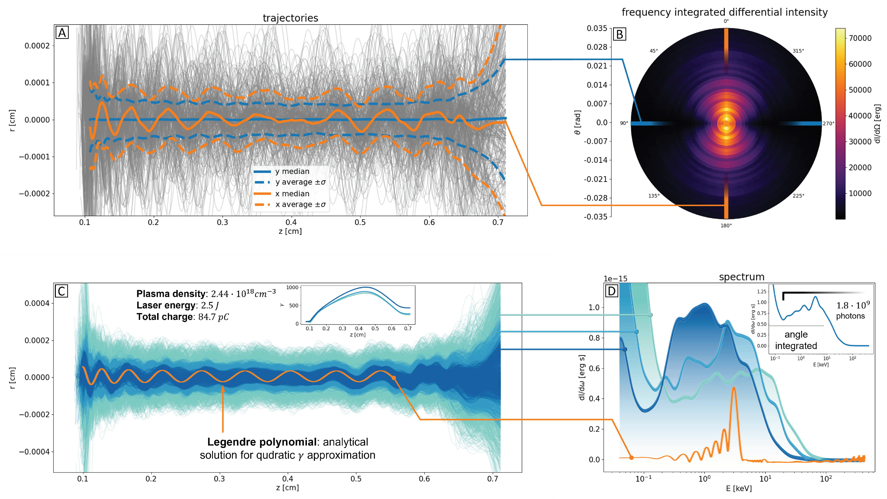
As a demonstration of the performance of the presented code, we showcase some results from the analysis of betatron radiation emitted by a self-injected electron beam during an LWFA shot simulated with FBPIC. The case involves a plasma density

n_{p} = 2.44 \times 10^{18} c m^{- 3}

and a laser pulse energy

E_{l} = 2.5 J

. Other relevant laser pulse parameters, common to all simulations, include the wavelength

λ_{l} = 800 n m

, temporal length

τ_{l} = 25 f s

, and beam waist

w_{l} = 15 μ m

, assuming a perfectly Gaussian transverse spot. The laser pulse is polarized along the

\hat{x}

axis. In this instance, 10000 macroparticles were self-injected, and 600 timesteps of the PIC simulation were selected, requiring a computation time of

30 m i n

for a total of 100 different detector positions. Figure 5 visually represents the analysis of the presented case. In panel

5 A

, the trajectories

x - z

of the selected self-injected beam are shown in gray, the median of the x coordinate (y coordinate) as a function of z is depicted in full orange (blue), and the corresponding mean

\mp σ

(standard deviation) is shown in dashed lines. A clear collective oscillation of the beam along the

\hat{x}

axis is observed, which coincides with the laser’s polarization. Whether this behavior is an isolated occurrence or a systematic feature and whether it is a physical characteristic or a PIC numerical artifact are aspects currently under evaluation. Nonetheless, if this characteristic proves to be genuine and controllable, it could provide significant advantages in terms of resulting field intensity and photon flux.

In panel

5 B

, the intensity of total radiation (integrated over all selected frequencies corresponding to the range

10^{- 1} - 10^{2} k e V

) is represented in color-coded variable on the angular spot centered along the laser propagation axis: the differences in intensity and radiation divergence along the two axes confirm what was mentioned about the trajectories in panel

5 A

. In panel

5 C

, a more detailed analysis of the beam was performed by dividing the particles into three chunks (represented by three shades of blue) based on their similarity with the oscillating median in panel

5 A

. The subfigure on the top shows the average

γ

of the particles in each chunk as a function of z. The core of the beam (dark blue) exhibits an initial clear collective oscillation along the

\hat{x}

axis (on the left), which gradually fades due to a dephasing process and reappears partially in the final part (on the right). In orange, an analytical trajectory is overlaid, calculated assuming a parabolic energy profile obtained from a fit of the average

γ

reported in the subfigure. It shows a good agreement with the initial and final sections of the trajectories, demonstrating that the core moves approximately like a single ideal electron. It can be demonstrated that in the case of parabolic longitudinal acceleration, the analytical trajectory for an electron subjected to a linear focusing transverse force is approximated by a linear combination of Legendre polynomials. A dedicated work focused on this type of analysis, aimed at obtaining an approximate analytical expression of the spectrum, is currently under development. Finally, in panel

5 D

, the spectra emitted on-axis by each of the three isolated chunks in panel

5 C

are shown, along with the numerical spectrum calculated from the analytical trajectory (orange). In the top-right inset, the total spectrum integrated over solid angle is presented. Moving from light blue to dark blue, three effects can be observed:

Decrease in the cutoff energy.
Decrease in the extension of the low-energy background (left).
Increase in peak intensity.

The first effect can be attributed to the progressive reduction in the trajectories average amplitude: experiencing less acceleration (recall that transverse force is linear with distance from axis), the related emitted radiation will be less energetic. The second and third effects seem to be related to the increased coherence and energy as one moves towards the core: a more coherent oscillation will enhance total intensity, while the concurrent reduction of noise will give a neater spectrum profile. Finally, although the (scaled for comparison) spectrum associated with the analytical trajectory (orange) shows different characteristics due to the evident simplification of the system, the energy extension remains consistent, particularly with that of the spectrum associated with the core trajectories (dark blue).

4. Conclusions

The code presented, specifically developed for calculating betatron radiation spectra within the EuAPS project, is suited for the calculation of radiation emission from any set of particle trajectories whose energy greatly exceeds that of the radiation itself (i.e. radiation recoil is not included). So far, trajectories obtained from PIC calculations are employed to compute delayed fields radiation on a detector. These fields are then Fourier transformed to retrieve the spectrum. The forward delayed fields calculation approach, presented in subSection 2.2, enables direct integration into any PIC (Particle-in-Cell) code, easing data management and extracting all possible trajectories’ information for spectrum calculation. The code was validated through analytical undulator spectra comparison ad it’s currently used on a daily base in a parametric scan of laser-plasma parameters process. A systematic evaluation of calculated intensity scaling for different levels of undersampling may also enable a quick and approximate usage based on a few trajectory points, providing an order of magnitude estimation of the number of produced photons.

Funding

This work has been partially funded by European Union - Next Generation EU.

Data Availability Statement

Data available on request to main author’s mail addresses.

References

Assmann, R. W.; Ferrario, M. et al. EuPRAXIA Advanced Photon Sources PNRR_EuAPS Project, 2023.
Assmann, R. W.; Ferrario, M. et al. EuPRAXIA Conceptual Design Report; Springer Science and Business Media LLC, 2020. [CrossRef]
Esarey, E.; Shadwick, B. A.; Catravas, P.; Leemans, W. P. Synchrotron radiation from electron beams in plasma-focusing channels; APS, 2002. [CrossRef]
Kostyukov, I.; Kiselev, S.; Pukhov, A. X-ray generation in an ion channel; AIP, 2003. [CrossRef]
Paroli, B.; Potenza, M. A. C. Radiation emission processes and properties: synchrotron, undulator and betatron radiation; Editor: Informa UK Limited, 2017. [CrossRef]
FBPIC (Fourier-Bessel Particle-In-Cell) documentation: https://fbpic.github.io/.
Lehe, R.; Kirchen, M.; Andriyash, I. A.; Godfrey, B. B.; Vay, J. A spectral, quasi-cylindrical and dispersion-free Particle-In-Cell algorithm; Computer Physics Communications, 2016. [CrossRef]
Jackson, J. D. Radiation from Moving Charges. In Classical electrodynamics, 2nd ed.; Editor: Wiley, 1975.
Smilei documentation: https://smileipic.github.io/Smilei/.
Ciocci, F. ; Dattoli, G.; Renieri, A.; Torre, A. Generalities on Synchrotron Radiation. In Insertion Devices For Synchrotron Radiation And Free Electron Laser; Editor: World Scientific Publishing Company, 2000.

Figure 1. Three steps of the alignment loop for variables in sorted arrays.

A_{c}

advances only when and where there is a match between the current ID and the local IDs. The variables in

A_{f i n}

are updated (light blue) with the corresponding values extracted from

A_{t e m p}

(light green). Note that the number of columns in

A_{t e m p}

and

A_{f i n}

is not generally the same.

Figure 1. Three steps of the alignment loop for variables in sorted arrays.

A_{c}

advances only when and where there is a match between the current ID and the local IDs. The variables in

A_{f i n}

are updated (light blue) with the corresponding values extracted from

A_{t e m p}

(light green). Note that the number of columns in

A_{t e m p}

and

A_{f i n}

is not generally the same.

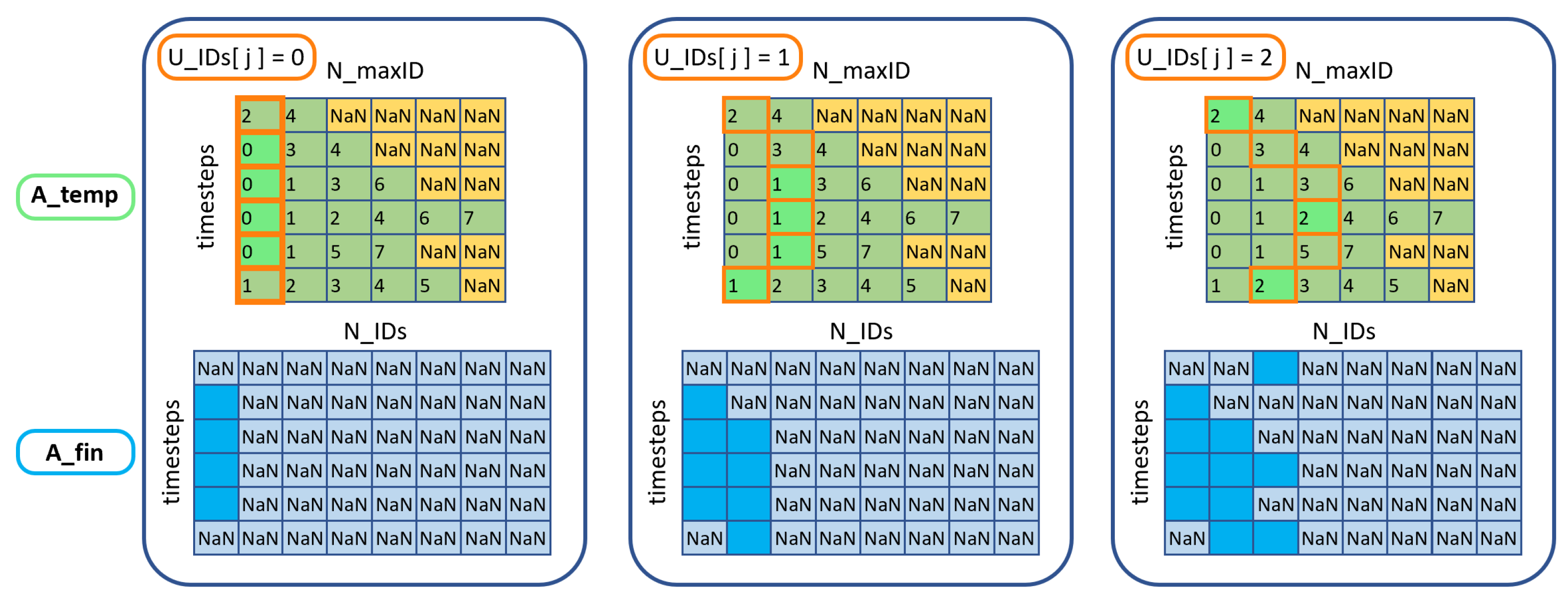
Figure 2. Space-time diagrams for delayed field usage patterns. The detector’s position is shown in dashed orange, the particle’s trajectory in solid green, and the light cones of the signals in continuous black at 45° angles. (a) Backward approach, evenly spaced times on the detector, requiring interpolation along the trajectory. Given the highly relativistic regime, this could easily lead to causality violation. (b) Forward approach, evenly spaced times along the trajectory, resulting in irregular times on the detector. Causality is always preserved.

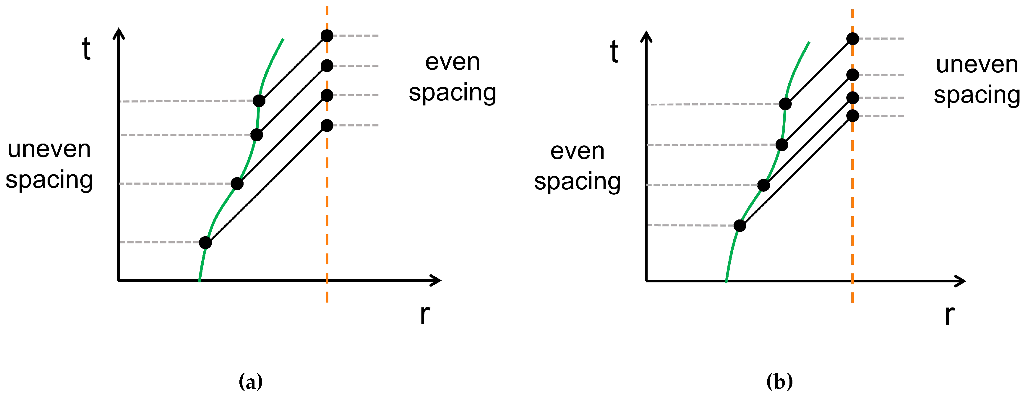
Figure 3. Schemes for total spectrum calculation through Fourier transform. (a) Visual schematization of the TFC and DFC approaches. Broken lines of different colors represent the fields calculated by different particles. The shaded yellow line represents the total field at the detector. (b) Performance analysis of the two approaches as a function of the number of particles analyzed, based on the convergence of the mean squared error with respect to the polynomial degree of the runtime fit. For TFC, the effect of sorting and summing an increasing number of arrays composed of a growing number of elements results in an overall quadratic scaling. Conversely, for DFC, the expected and measured scaling is linear.

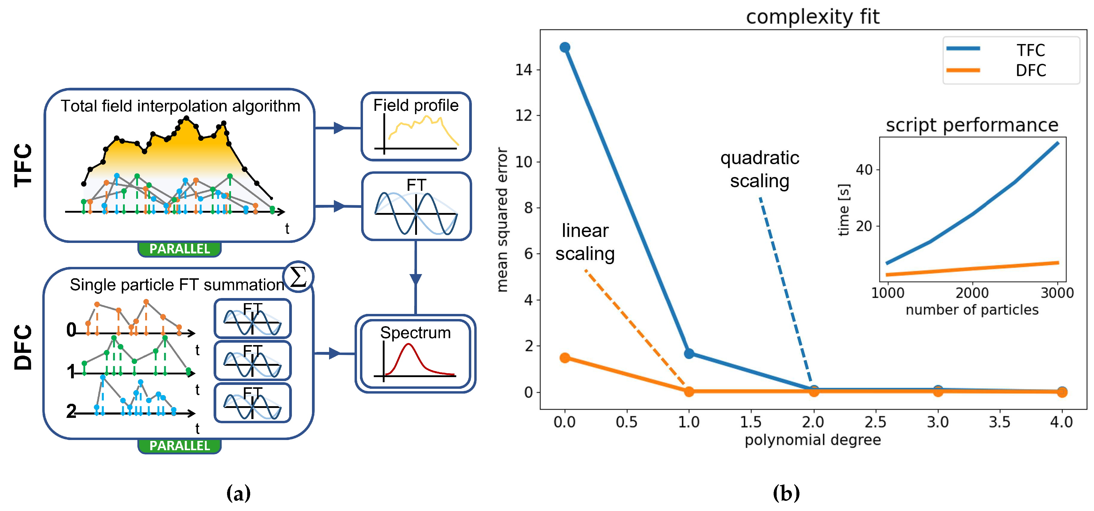
Figure 4. Comparison between numerical spectra (full lines) and analytical spectra (dashed lines) along with the evaluation of the theoretical position of the first harmonic (vertical dashed lines) for an electron in an undulator. Evaluations were performed for several values of the undulator strength K, and the on-axis spectra for

K = 0.3

and

K = 3

are shown in panels (a) and (b) respectively.

K = 0.3

and

K = 3

are shown in panels (a) and (b) respectively.

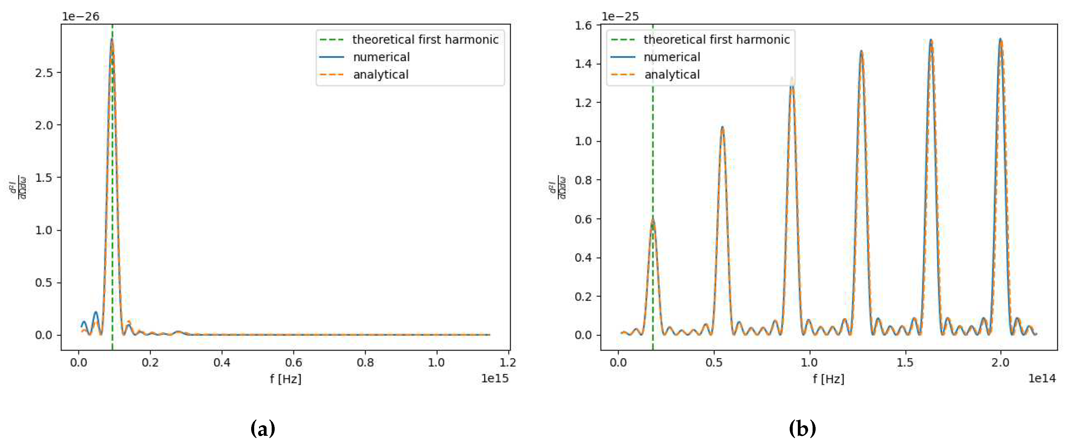
Figure 5. Analysis of betatron radiation spectrum emitted by a PIC-simulated LWFA self-injected beam. (A) Trajectories

x - z

of the beam, with medians and means

\mp σ

along the two transverse axes (

\hat{x}

and

\hat{y}

). (B) Radiation intensity on angular spot. (C) Division of beam particles into three chunks based on their similarity level with the median along the

\hat{x}

axis; superimposed: analytical trajectory of a single electron with quadratically approximated acceleration (orange). (D) Spectra of the three chunks from figure (C) along with the (scaled) numerical spectrum of the analytical trajectory (orange) and the total spectrum integrated over the solid angle (top right).

Figure 5. Analysis of betatron radiation spectrum emitted by a PIC-simulated LWFA self-injected beam. (A) Trajectories

x - z

of the beam, with medians and means

\mp σ

along the two transverse axes (

\hat{x}

and

\hat{y}

). (B) Radiation intensity on angular spot. (C) Division of beam particles into three chunks based on their similarity level with the median along the

\hat{x}

Disclaimer/Publisher’s Note: The statements, opinions and data contained in all publications are solely those of the individual author(s) and contributor(s) and not of MDPI and/or the editor(s). MDPI and/or the editor(s) disclaim responsibility for any injury to people or property resulting from any ideas, methods, instructions or products referred to in the content.

© 2023 by the authors. Licensee MDPI, Basel, Switzerland. This article is an open access article distributed under the terms and conditions of the Creative Commons Attribution (CC BY) license (http://creativecommons.org/licenses/by/4.0/).

Copyright: This open access article is published under a Creative Commons CC BY 4.0 license, which permit the free download, distribution, and reuse, provided that the author and preprint are cited in any reuse.

Submitted:

12 October 2023

Posted:

13 October 2023

You are already at the latest version

Alerts

Abstract

Keywords:

Subject: Physical Sciences - Applied Physics

1. Introduction

2. Materials and Methods

2.1. Data Structuring

γ

The proposed approach involves inserting the data into at least two-dimensional arrays with dimensions

[N_{t i m e s t e p} \times N_{I D s}]

, where

N_{t i m e s t e p}

is the number of timesteps in the PIC simulation, and

N_{I D s}

is the number of unique particle IDs: these arrays will be called

A_{f i n}

as they are the final data format. For vector quantities such as position and momentum, the arrays will be of size

[N_{t i m e s t e p} \times N_{I D s} \times 3]

A_{f i n}

will be performed using temporary arrays

A_{t e m p}

of smaller dimensions

[N_{t i m e s t e p} \times N_{m a x I D}]

. Here,

N_{m a x I D}

represents the maximum instantaneous size of the self-injected beam, in terms of particle number. This step will facilitate an orderly extraction of variables.

The data structuring takes place in the following steps:

First loop over the timesteps to identify the maximum number of concurrent IDs $N_{m a x I D}$ in a single timestep (maximum instantaneous "size" of the self-injected beam).
Identification of the array of unique IDs $U_{I D s}$ , with size $N_{I D s} \geq N_{m a x I D}$ .
Creation of temporary arrays $A_{t e m p}$ with dimensions $[N_{t i m e s t e p} \times N_{m a x I D}]$ or $[N_{t i m e s t e p} \times N_{m a x I D} \times 3]$ .
Second loop over the timesteps, sorting the variables by ID values, and inserting them into the $A_{t e m p}$ arrays. Note that in a timestep (row of $A_{t e m p}$ ), the number of present IDs may generally be $< N_{m a x I D}$ . In these cases, the variables sorted by ID will be accumulated in the leftmost columns of $A_{t e m p}$ , while NaNs will be left in the free cells. (see leftmost block in Figure 1, green/yellow array matrix)
Creation of final arrays $A_{f i n}$ filled with NaN values, with dimensions $[N_{t i m e s t e p} \times N_{I D s}]$ or $[N_{t i m e s t e p} \times N_{I D s} \times 3]$ (see leftmost block in Figure 1, blue array matrix).
ID alignment: a single loop with index (j) over $U_{I D s}$ . A counter array $A_{c}$ with size $N_{t i m e s t e p}$ is incremented only at positions i where ${I D_{t e m p}}^{i, A_{c}} = {U_{I D s}}^{j}$ . The same indices for which this condition is satisfied are used to extract the variables from $A_{t e m p}$ and insert them into $A_{f i n}$ . A visual representation of the loop is presented in Figure 1, going from left box to the right one.

In this way, the array

A_{f i n}

A_{c}

, which adapts to the non-uniformity of particle IDs original distribution (see orange boxed cells in green/yellow array matrices in Figure 1, evolving from left to right): where

A_{c}

finds the "right" ID cells in

A_{t e m p}

(highlighted green in figure), the algorithm assigns the corresponding values to a single column in

A_{f i n}

2.2. Spectrum calculation

\vec{E} (\vec{r}, t) = e {[\frac{\vec{n} - \vec{β}}{γ^{2} {(1 - \vec{β} \cdot \vec{n})}^{3} R^{2}}]}_{r e t} + \frac{e}{c} {[\frac{\vec{n} \times ((\vec{n} - \vec{β}) \times \dot{\vec{β}})}{{(1 - \vec{β} \cdot \vec{n})}^{3} R}]}_{r e t}

(1)

where e is the charge of the electron, c is the speed of light,

γ

is the Lorentz factor, R is the distance between the trajectory and the detector,

\vec{n}

is the unit vector pointing from the trajectory to the detector, and

\vec{β}

and

\dot{\vec{β}}

are the velocity and acceleration of the particle normalized to c. Note that the given expression is valid in CGS units. Then, defining the quantity

\vec{A} (\vec{r}, t) = {(\frac{c}{4 π})}^{\frac{1}{2}} {[R \vec{E}]}_{r e t}

(2)

and performing its Fourier transform on the detector

\vec{A} (\vec{r}, ω) = \frac{1}{\sqrt{2 π}} \int \vec{A} (\vec{r}, t) e^{- i ω t} d t

(3)

the differential intensity over frequency

ω

and solid angle

Ω

is obtained as follows

\frac{d^{2} I}{d Ω d ω} = 2 {| \vec{A} (\vec{r}, ω) |}^{2}

(4)

where the dimensions of the last expression is [erg s]. In Eq.1 and Eq.2, the subscript

r e t

indicates that the field at point

\vec{r}

at time t must be evaluated by finding an appropriate value of R that provides an intersection between the back-propagating light cone from point

(\vec{r}, t)

and the trajectory of the particle. The values of the variables necessary for the field calculation should then be evaluated at time

t - R / c

, taking into account the signal propagation at velocity c. This conventional "backward" approach allows us to

s e l e c t

a grid of times

t_{d}

at which to evaluate the field on the detector and requires interpolating the trajectory at the points indicated by the reasoning just described, thus

d e r i v i n g

a grid of times on the trajectory

t_{t}

(Figure 2 a). In the case of relativistic particles, interpolating the trajectories is a delicate and potentially risky operation, as even small variations in quantities like

\vec{β}

and

\dot{\vec{β}}

c h o o s i n g

a grid of times on the trajectory

t_{t}

and

d e r i v i n g

a grid of times on the detector

t_{d}

. Given the distance R between trajectory and detector at each instant, the fields calculated with Eq.1 will be associated with the time

t_{d} = t_{t} + R / c

(Figure 2 b).

t_{t, 2} = t_{t, 1}

) would result in different arrival times of the signal on the detector compared to those produced by the first trajectory (

t_{d, 2} \neq t_{d, 1}

) due to the particles’ different positions. Furthermore, changing the position of the detector may also alter the order in which the elements of

t_{d, 2}

and

t_{d, 1}

alternate. Thus, two approaches to spectrum calculation are outlined, each with different computational complexities and different levels of extracted information (Figure 3):

1.

all the fields on the detector are combined into a single array, which is then sorted based on $t_{d, a l l}$
concurrently, a container of size $t_{d, a l l}$ is filled by interpolating the field of each particle i at all the missing time points $t_{d, a l l - i}$
finally, the ordered fields from the first step are directly summed into the container, providing the temporal profile of the total field

Then to compute the spectrum it is possible to perform a Fourier Transform (FT) directly on the total field on the detector, using

t_{d, a l l}

as the array of times.

2.

3. Results

1 - 10 k e V

d^{2} I / d Ω d ω

3.1. Validation

\frac{d^{2} I}{d Ω d ω} = \frac{e^{2} N^{2} γ^{2}}{c} \sum_{m = 1}^{\infty} F_{m} (ξ) s i n c^{2} (ν_{m} / 2)

(5)

where

ξ

is a variable defined from the undulator force,

F_{m} (ξ)

is a function composed of Bessel functions of the first kind,

ν_{m}

is a linear variable of frequency

ω

1 / γ

1 / γ

. Let’s assume that the transverse coordinate x as a function of the longitudinal coordinate z is approximately

x (z) = \frac{K}{k_{U} γ} c o s (k_{U} z)

(6)

with K undulator strength and

k_{U}

undulator wavevector. Then, the angle of the tangent to the trajectory will be given by

θ = \frac{d x}{d z} = - \frac{K}{γ} s i n (k_{U} z) \approx - \frac{K k_{U}}{γ} z

(7)

Calculating from Eq. 7, the

Δ θ

as a function of the

Δ z

of the trajectory and equating it to

1 / γ

, it is possible to determine the

Δ t

of the trajectory generating a visible signal on the detector by substituting the velocity

v = β c

Δ z = \frac{1}{K k_{U}} Δ t \approx \frac{1}{K k_{U} β c}

(8)

It has been verified that by choosing a timestep sufficiently smaller than the one indicated by the condition given by Eq.8 (e.g.

Δ t_{s i m} = 0.1 Δ t

), the oscillation of the field on the detector is correctly reconstructed, and there is a coincidence between the theoretical and numerically calculated spectra. For larger

Δ t_{s i m}

3.2. Betatron radiation analysis: a peculiar case

n_{p} = 2.44 \times 10^{18} c m^{- 3}

and a laser pulse energy

E_{l} = 2.5 J

. Other relevant laser pulse parameters, common to all simulations, include the wavelength

λ_{l} = 800 n m

, temporal length

τ_{l} = 25 f s

, and beam waist

w_{l} = 15 μ m

, assuming a perfectly Gaussian transverse spot. The laser pulse is polarized along the

\hat{x}

axis. In this instance, 10000 macroparticles were self-injected, and 600 timesteps of the PIC simulation were selected, requiring a computation time of

30 m i n

for a total of 100 different detector positions. Figure 5 visually represents the analysis of the presented case. In panel

5 A

, the trajectories

x - z

of the selected self-injected beam are shown in gray, the median of the x coordinate (y coordinate) as a function of z is depicted in full orange (blue), and the corresponding mean

\mp σ

(standard deviation) is shown in dashed lines. A clear collective oscillation of the beam along the

\hat{x}

In panel

5 B

, the intensity of total radiation (integrated over all selected frequencies corresponding to the range

10^{- 1} - 10^{2} k e V

5 A

. In panel

5 C

, a more detailed analysis of the beam was performed by dividing the particles into three chunks (represented by three shades of blue) based on their similarity with the oscillating median in panel

5 A

. The subfigure on the top shows the average

γ

of the particles in each chunk as a function of z. The core of the beam (dark blue) exhibits an initial clear collective oscillation along the

\hat{x}

γ

5 D

, the spectra emitted on-axis by each of the three isolated chunks in panel

5 C

Decrease in the cutoff energy.
Decrease in the extension of the low-energy background (left).
Increase in peak intensity.

4. Conclusions

Funding

This work has been partially funded by European Union - Next Generation EU.

Data Availability Statement

Data available on request to main author’s mail addresses.

References

Assmann, R. W.; Ferrario, M. et al. EuPRAXIA Advanced Photon Sources PNRR_EuAPS Project, 2023.
Assmann, R. W.; Ferrario, M. et al. EuPRAXIA Conceptual Design Report; Springer Science and Business Media LLC, 2020. [CrossRef]
Esarey, E.; Shadwick, B. A.; Catravas, P.; Leemans, W. P. Synchrotron radiation from electron beams in plasma-focusing channels; APS, 2002. [CrossRef]
Kostyukov, I.; Kiselev, S.; Pukhov, A. X-ray generation in an ion channel; AIP, 2003. [CrossRef]
Paroli, B.; Potenza, M. A. C. Radiation emission processes and properties: synchrotron, undulator and betatron radiation; Editor: Informa UK Limited, 2017. [CrossRef]
FBPIC (Fourier-Bessel Particle-In-Cell) documentation: https://fbpic.github.io/.
Lehe, R.; Kirchen, M.; Andriyash, I. A.; Godfrey, B. B.; Vay, J. A spectral, quasi-cylindrical and dispersion-free Particle-In-Cell algorithm; Computer Physics Communications, 2016. [CrossRef]
Jackson, J. D. Radiation from Moving Charges. In Classical electrodynamics, 2nd ed.; Editor: Wiley, 1975.
Smilei documentation: https://smileipic.github.io/Smilei/.
Ciocci, F. ; Dattoli, G.; Renieri, A.; Torre, A. Generalities on Synchrotron Radiation. In Insertion Devices For Synchrotron Radiation And Free Electron Laser; Editor: World Scientific Publishing Company, 2000.

Figure 1. Three steps of the alignment loop for variables in sorted arrays.

A_{c}

advances only when and where there is a match between the current ID and the local IDs. The variables in

A_{f i n}

are updated (light blue) with the corresponding values extracted from

A_{t e m p}

(light green). Note that the number of columns in

A_{t e m p}

and

A_{f i n}

is not generally the same.

Figure 1. Three steps of the alignment loop for variables in sorted arrays.

A_{c}

advances only when and where there is a match between the current ID and the local IDs. The variables in

A_{f i n}

are updated (light blue) with the corresponding values extracted from

A_{t e m p}

(light green). Note that the number of columns in

A_{t e m p}

and

A_{f i n}

is not generally the same.

K = 0.3

and

K = 3

are shown in panels (a) and (b) respectively.

K = 0.3

and

K = 3

are shown in panels (a) and (b) respectively.

Figure 5. Analysis of betatron radiation spectrum emitted by a PIC-simulated LWFA self-injected beam. (A) Trajectories

x - z

of the beam, with medians and means

\mp σ

along the two transverse axes (

\hat{x}

and

\hat{y}

). (B) Radiation intensity on angular spot. (C) Division of beam particles into three chunks based on their similarity level with the median along the

\hat{x}

Figure 5. Analysis of betatron radiation spectrum emitted by a PIC-simulated LWFA self-injected beam. (A) Trajectories

x - z

of the beam, with medians and means

\mp σ

along the two transverse axes (

\hat{x}

and

\hat{y}

). (B) Radiation intensity on angular spot. (C) Division of beam particles into three chunks based on their similarity level with the median along the

\hat{x}

MDPI Initiatives

Important Links

Choose an area of interest and we will send you notifications of new preprints at your preferred frequency.

Disclaimer

First Simulations for the EuAPS Betatron Radiation Source

Abstract

1. Introduction

2. Materials and Methods

2.1. Data Structuring

2.2. Spectrum calculation

3. Results

3.1. Validation

3.2. Betatron radiation analysis: a peculiar case

4. Conclusions

Funding

Data Availability Statement

References

Abstract

1. Introduction

2. Materials and Methods

2.1. Data Structuring

2.2. Spectrum calculation

3. Results

3.1. Validation

3.2. Betatron radiation analysis: a peculiar case

4. Conclusions

Funding

Data Availability Statement

References

MDPI Initiatives

Important Links

Subscribe