Submitted:
16 October 2023
Posted:
16 October 2023
You are already at the latest version
Abstract
Liquidity providers for asset-pair pools with constant value distri- bution, such as Balancer pools, experience some impermanent loss whenever there is price divergence in the tokens’ fiat values. In this paper, we model this impermanent loss for geometric mean invariant pools by deriving a function of two parameters. We analyze our function graphically, showing that unevenly distributed pools with large weighting disparities best mitigate the risk of impermanent loss. We conclude by providing a general protocol for liquidity providers to choose a suitable pool based on their risk tolerance and profit goals.
Keywords:
Impermanent Loss
; Liquidity Pools
; Geometric Mean Market Makers
; Optimization
; DeFi
MSC: Primary 91B74
1. Introduction
Automated Market Makers (AMMs) have revolutionized the cryptocurrency exchange landscape. AMMs provide an infrastructure for decentralized trading platforms that operate on predefined algorithms implemented through automated Smart Contracts rather than using the traditional order book system employed by centralized exchanges. Crucial to the decentralized finance (DeFi) paradigm is the concept of liquidity provision, where users can deposit assets into a liquidity pool, facilitating trade in return for earning a commission fee. Liquidity providers (LPs) who contribute to a pool face the risk of impermanent loss (IL), which refers to the loss experienced when the prices of assets in a pool diverge from their prices at the time of the LPs entry. Impermanent loss can be described quantitatively as the potential difference in value between holding assets in an AMM and simply holding them outside of a DeFi pool. Because IL is essentially the opportunity cost of liquidity provision versus holding cryptocurrencies outside of a pool, it is deemed ’impermanent’ until the LP withdraws their funds, at which point their loss becomes a ’realized’ divergence loss.
In this study, we consider liquidity pools comprised of only two tokens, called asset-pair liquidity pools. Various AMM protocols exist for ensuring the ratio of assets in a pool is maintained, though we will focus solely on pools utilizing a geometric mean invariant, such as Balancer pools. These pools utilize the following value function, which ensures that each token/cryptocurrency accounts for a constant share of the pool’s total value [4].
Where V is the invariant value function, t ranges the tokens in the pool, represents the quantity of token t in the pool, and is the constant weight of token t, such that .
Our goal is to elucidate the factors contributing to IL and provide guidance to LPs on how to optimize their strategies, considering potential asset price movements and their risk appetite. The ensuing sections will detail our methodologies, present our findings on pool compositions and their respective susceptibilities to IL, and conclude with actionable insights and best practices for LPs navigating the DeFi space.
2. Formula for Impermanent loss
For the purposes of this paper, we will assume there are no pool fees. Because geometric mean market makers have an Exchange Rate Level Independence property [5], we can consider impermanent loss in terms of price ratios rather than actual prices. As such, we can greatly reduce the required number of parameters to calculate impermanent loss. Consider the following general formula [3]:
Where is the fiat value of the pool, is the fiat valuation of the tokens had they been held outside of the pool, is the fiat price of token t, and is the weight of token t. This formula provides impermanent loss (as a percentage) for a complex pool with n tokens, requiring parameters. However, for our analysis of asset-pair pools, the formula can be rewritten for two tokens:
For ease of optimization and modeling, we will assume that only one token’s value is fluctuating. We will choose as our numeraire, and assume the fiat value of remains constant. Thus, , such that:
This equation allows us to express impermanent loss in terms of only two parameters, and . Because the sum of all token weights must add up to 1, we are able to calculate using . We will now provide a derivation for this formula. First, we will use the Exchange Rate Level Independence property to express the pool value in terms of token 1, beginning by establishing the spot price formula given in the Balancer whitepaper [4].
Definition 2.1.
Let be the quantity of token t in the pool. The spot price (exchange rate) of two tokens may be expressed as a ratio of their quantities divided by their weights. Let be the price of token t in terms of token 1:
We can equate the fiat value of the pool to the sum of each token’s fiat value times its quantity:
Using Definition 2.1, we can express the pool value in terms of token 1:
Note that simply equals 1. It follows that the pool’s fiat value can be expressed as the product of the pool value in terms of token 1 and the fiat value of token 1:
Such that:
Using Equation (2.6) and letting be the new value of the pool in terms of token 1, we can rewrite as:
Referring to Theorem 2.2 (at the end of the section), we know:
Substituting into Equation (2.9):
Notice the substitution of Equation (2.6) into Equation (2.12). Recall a property of Definition 2.1, such that . Continuing Equation (2.13):
As such, we have shown that the change in the pool’s value in terms of token 1 is equal to the change in token 2’s value in terms of token 1, raised to the power of token 2’s weight. Inserting this into Equation (2.8):
Recall . Thus:
This matches the expression for we set out to derive in Equation (2.2). To compute impermanent loss, we must now derive an expression for . Because there is a constant value distribution [4], we can express the total fiat value of the pool as such:
Since the tokens are being held outside the pool, we may express the new held fiat value as being directly proportional to the fiat price changes of the tokens:
As such:
We can now substitute Equation (2.17) and Equation (2.20) into Equation (2.1), yielding:
However, because we are modeling impermanent loss according to fluctuation of only one token’s fiat value, we let . Thus:
Rewriting in terms of yields a function of two parameters:
In Section 3, we will analyze this function further to determine which weighting scheme is optimal for reducing impermanent loss in asset-pair pools. We will now prove the expression for presented in Equation (2.10).
Theorem 2.2.
For any asset-pair liquidity pool with a geometric mean invariant and no trading fees, the future quantity of some token t after experiencing divergence in fiat price can be represented by the following equation:
Where is the original quantity of token t, is token t’s weighted value proportion in the pool, and is the change in token t’s value relative to token 1.
Proof.
Recall from Section 1 that the value function V remains constant throughout price variance. As such, the following holds true:
Now, let us divide both sides by a common term :
Recalling Definition 2.1, we can express as:
Substituting into Equation (2.25) and Equation (2.26):
Thus, our proof is complete. □
3. Analysis and Optimization
In this section, we will model the function derived in Section 2, shown in Equation (2.23), to get a graphical understanding of how to best optimize impermanent loss. We will calculate the optimal weight for token 1 at various values of , and use our findings to determine ideal pool weighting for varying volatility profiles.
Plotting IL as a function of reveals some important elementary qualities, shown in Figure 1a,b.
As expected, IL converges to 0 when is 1, as there is no IL experienced when the token price remains constant. The downward concavity of the IL function and maxima at make it clear that any price fluctuation (regardless of direction) creates some impermanent loss. Evidently, decreases in fiat value yield a greater impermanent loss than increases in fiat value of the same proportion. It also appears that pools with more even weight distributions experience larger proportions of impermanent loss than heavily skewed pools when price fluctuates. Recall the Exchange Rate Level Independence property we used to derive our IL function, which considers as a price change ratio rather than the true change in fiat value of token 1 (i.e. if token 1’s fiat value increases from $10 to $15, ).
Similarly, the y-axis (impermanent loss) represents a percentage decrease from the original fiat value held (i.e. IL = -0.2 means a 20% loss). Going beyond mathematical implications, let us consider the practical applications of the curves presented in Figure 1. A liquidity provider possessing more volatile coins with a higher likelihood of price divergence should certainly opt for an uneven pool (i.e. 80/20 weight distribution) to minimize their impermanent loss. New cryptocurrency projects frequently utilize uneven ratios via Liquidity Bootstrapping Pools, often providing large exposure to their token paired with a smaller share of some stablecoin (i.e. DAI) [2]. Considering the volatility of novel coins, employing a skewed weighting scheme greatly reduces the risk of large impermanent loss. We can see this clearly by modeling our function in three-space:
Values of around 0.5 have notably steep valleys as approaches values of extreme price fluctuation. Values of near 0 and 1 yield greater (meaning less impermanent loss) values of IL during extreme price fluctuation. Thus, a liquidity provider looking to minimize their risk should always select a non-central weighting scheme that values tokens’ share of the pool in a heavily skewed manner.
However, it is important to note that uneven pools have notably higher slippage rates [2]. Slippage is the price difference between quoted transaction price and actual transaction price upon confirmation, and results in traders receiving fewer tokens than expected for a swap. Generally, the farther token weighting is away from 50/50, the greater the amount of slippage incurred by traders [2]. While not directly harmful to liquidity providers, high slippage results in fewer pool trades, and thus produces lower trading fee returns for LPs [2]. As such, LPs should consider both their risk tolerance and profit expectations when selecting a liquidity pool.
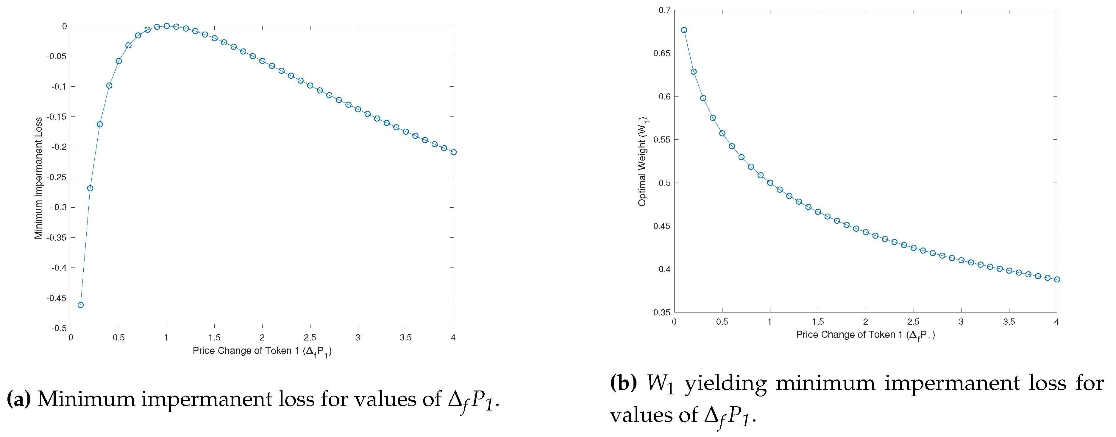
The sensitivity analysis shown above in Figure 3 shows that impermanent loss is highly sensitive to price fluctuation, particularly when price is decreasing. The trend shown in Figure 3 illustrates clearly that an IL from a decrease in token 1’s price is best mitigated by a large pool share of token 1, while the inverse is true for an increase of token 1’s fiat price. It follows that an LP who believe some token t will increase in fiat value should invest in pools with a large stablecoin share and a small share of token t.
With this in mind, let us conclude with some best practices for LPs looking to minimize their risk in asset-pair pools. To preface, these practices are only practical in application to non-stablecoin pairs. Pools comprised entirely of stablecoins should use a dynamic stableswap invariant such as Curve’s Stableswap protocol, which is far more effective at reducing IL than a geometric mean invariant [1]. Based on our findings, it is clear that an LP looking solely to minimize their risk and loss should invest in an uneven pool with some 80/20 or larger weight disparity. However, a LP looking to balance risk and reward should select a more evenly distributed pool (i.e. 60/40) to increase profits with less slippage while still making efforts to mitigate IL. If an LP is bullish on a token, they should invest in pools which have lower value shares of the token so that IL is minimized when the token value increases. The inverse is true as well, as tokens subject to high volatility should be weighted heavily in the pool to limit IL risk from price decrease. As such, we have established a clear protocol for liquidity providers to follow dependent on their risk tolerance, profit goals, and predictions for a token’s future price action.
Acknowledgments
The substitution outlined in Theorem 2.2 was inspired by a paper written by Fernando Martinelli on calculating the value of a Balancer pool. The paper, which was previously uploaded on Balancer’s website, is no longer available online.
References
- Egorov, M., (2019). StableSwap - efficient mechanism for Stablecoin liquidity. https://classic.curve.fi/files/stableswap-paper.pdf.
- Martinelli, F., (2020). 80/20 Balancer Pools. https://medium.com/balancer-protocol/80-20-balancer-pools-ad7fed816c8d.
- Martinelli, F. (2020). Calculating Value, Impermanent Loss and Slippage for Balancer Pools. https://medium.com/balancer-protocol/calculating-value-impermanent-loss-and-slippage-for-balancer-pools-4371a21f1a86.
- Martinelli, F., & Mushegian, N. (2019). Whitepaper: A non-custodial portfolio manager, liquidity provider, and price sensor. https://balancer.fi/whitepaper.pdf.
- Tiruviluamala, N., Port, A., & Lewis, E. (2022). A General Framework for Impermanent Loss in Automated Market Makers. [CrossRef]
Figure 1.
Model of impermanent loss as a function of for various values of .
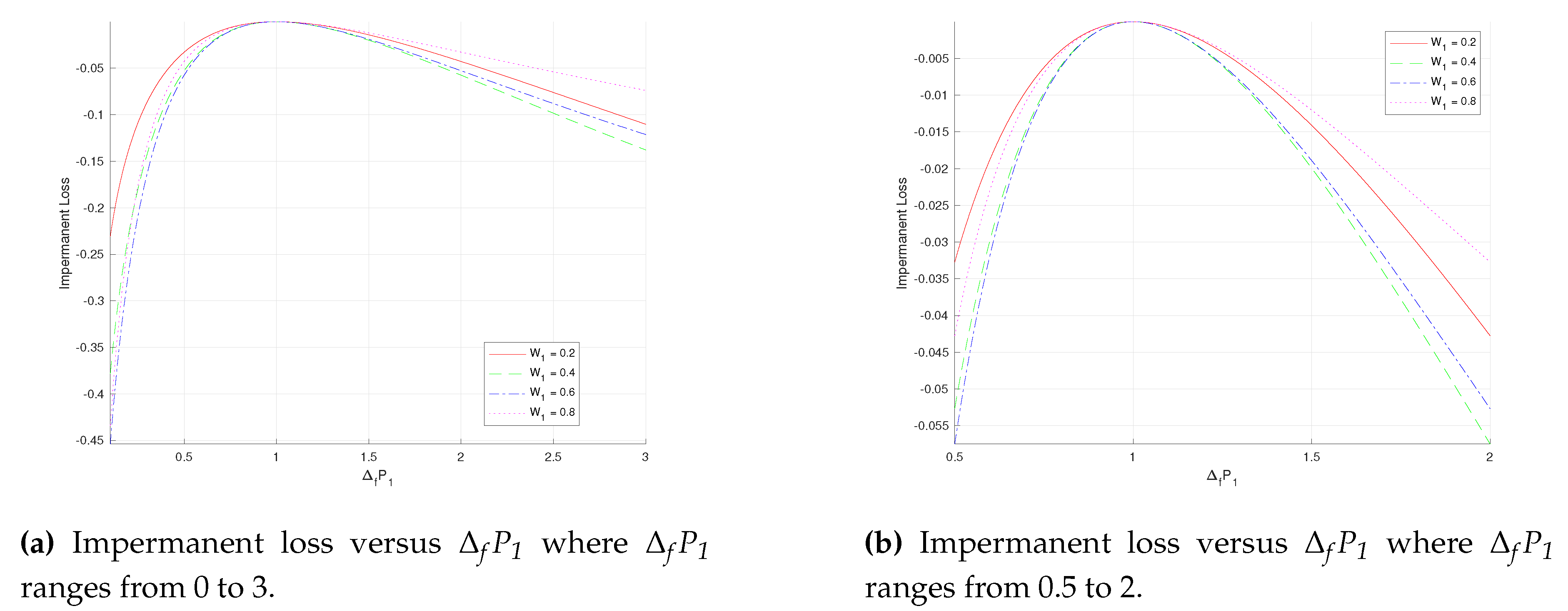
Figure 2.
Surface generated by
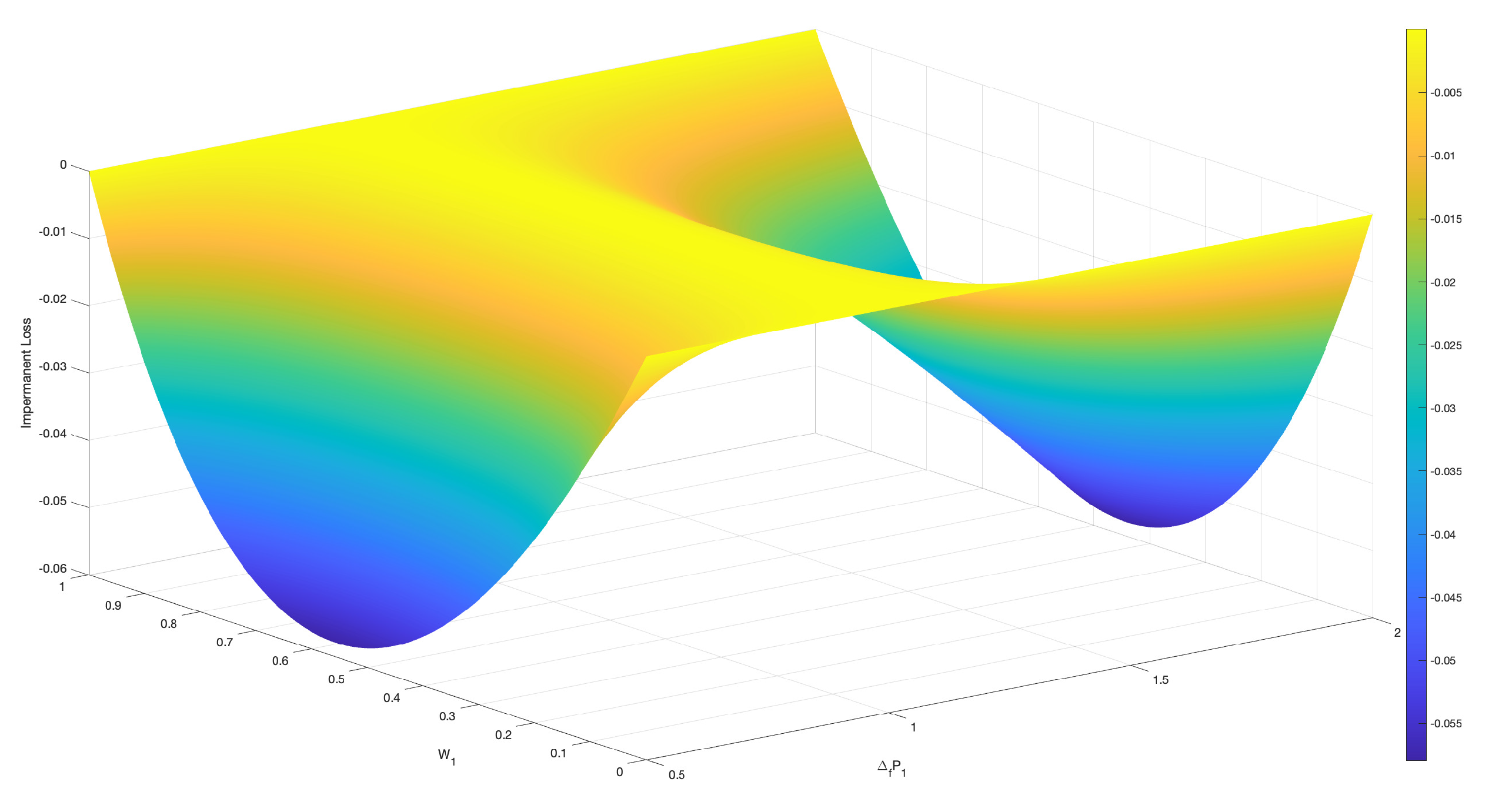
Figure 3.
Minimum impermanent loss for select price fluctuations and the corresponding value which achieves this.
Figure 3.
Minimum impermanent loss for select price fluctuations and the corresponding value which achieves this.
Disclaimer/Publisher’s Note: The statements, opinions and data contained in all publications are solely those of the individual author(s) and contributor(s) and not of MDPI and/or the editor(s). MDPI and/or the editor(s) disclaim responsibility for any injury to people or property resulting from any ideas, methods, instructions or products referred to in the content. |
© 2023 by the authors. Licensee MDPI, Basel, Switzerland. This article is an open access article distributed under the terms and conditions of the Creative Commons Attribution (CC BY) license (http://creativecommons.org/licenses/by/4.0/).
Copyright: This open access article is published under a Creative Commons CC BY 4.0 license, which permit the free download, distribution, and reuse, provided that the author and preprint are cited in any reuse.


