1. Introduction
The primary source of CO
2 in non-industrial indoor environments is human metabolism, resulting in higher concentrations compared to outdoor spaces [
1,
2]. It has been established that exposure to concentrations exceeding 1000 ppm can adversely affect human cognitive abilities [
3]. Additionally, CO
2 levels are closely linked to ventilation efficiency [
4] and the risk of indoor airborne infections [
5]. Due to these critical implications, CO
2 concentration is frequently employed as an indicator of indoor air quality.
Presently, a wide range of devices is available for measuring indoor CO
2 levels, with some capable of monitoring additional parameters such as relative humidity and temperature. These devices can be categorized into two groups: those that exclusively display real-time measurements, often via a screen, and those that offer data storage capabilities. Devices in the first group often include audible and visual alarms; nevertheless, they lack the capacity for generating historical records of measured variables. Devices in the second group allow for the storage of acquired data, typically through cloud servers managed by the manufacturing or marketing company [
6,
7].
In many cases, the acquisition of data for indoor air quality and environmental variables lacks the ability for total, unique, and personalized control, leading to limitations in understanding and responding to the data effectively. Additionally, data storage often comes with an extra cost, making long-term monitoring challenging.
Continuous monitoring over an extended period, ideally spanning several weeks, is essential for gaining a deeper insight into usage patterns, occupancy profiles, contamination types (background or localized), periodicity, and the potential for space improvement [
8,
9,
10].
In situations where thermal and humidity comfort is inadequate, it becomes necessary to assess and adjust the air conditioning system, control and regulation mechanisms, the need for humidification or dehumidification, and even calculate the required water vapor adjustments to achieve specific comfort conditions. This process enables the selection of appropriate devices or systems for this purpose. Monitoring CO
2 concentration and temperature is instrumental in evaluating the efficiency of ventilation systems and programming their regulation based on CO
2 levels [
3,
11,
12]. By addressing these aspects, this research aims to provide valuable insights and solutions for enhancing indoor air quality and environmental conditions in enclosed spaces.
1.1. Related Works
Over the past decade, significant advancements have been made in the field of weather prediction, driven by the application of advanced machine learning techniques. When it comes to analyzing time series datasets, such as signals and text, Long Short-Term Memory (LSTM) neural networks have emerged as a prominent choice [
13]. LSTM addresses a common challenge faced by Recurrent Neural Networks (RNN), which is the vanishing gradient problem, by incorporating memory cells and gating mechanisms. This unique architecture empowers LSTMs to effectively capture long-term dependencies within time series data, making them well-suited for tasks involving temporal patterns [
14].
Empirical evidence has demonstrated that LSTM architectures often outperform alternative machine learning models in terms of accuracy, particularly when dealing with numerical values.
Artificial Neural Networks (ANN) are intricate systems composed of interconnected processing units that operate in parallel. While ANNs have demonstrated excellent performance in applications like Optical Character Recognition (OCR), their superiority over traditional statistical pattern classifiers remains inconclusive [
15].
In ANN systems, the initial stage involves processing real-number input signals. The connections, often referred to as edges, link artificial neurons to their respective outputs and are determined by non-linear functions applied to the sum of their inputs. These edges have adjustable weights that evolve iteratively during the learning process, directly influencing the strength of the signal. For a signal to propagate from one layer to another within the ANN, it must surpass a predefined threshold. Typically, ANNs incorporate multiple layers to facilitate various transformations of input signals. After traversing these layers iteratively, the output layer produces the final results [
16].
Numerous previous studies have explored various ANN architectures [
17], applied LSTM for weather forecasting [
14], and developed simulation models to predict rainfall [
18], all of which have contributed to improved modeling efficiency. Additionally, research has been conducted to harness LSTM for greenhouse climate modeling, with a focus on forecasting the impact of six climate factors: temperature, light, humidity, CO
2 concentration, soil temperature, and soil moisture, on crop growth. To capture climate variations, a sliding time window approach was adopted to record minute-by-minute changes in environmental conditions. This model was evaluated using datasets comprising three different types of vegetables and demonstrated commendable accuracy when compared to alternative models. Notably, it exhibited robustness and optimal performance within a fixed 5-minute time window. However, the model's performance gradually declined as the window size was increased [
19].
In previous research [
20,
21], LSTM-based models have been successfully employed for a range of applications, including the prediction of Point of Interest (POI) categories and the hourly daily irradiance forecast. The solar prediction technique introduced in these studies, which combines LSTM with weather data, considers the interdependence of hours throughout the day. Results have demonstrated that this novel approach exhibits reduced overfitting and superior generalization capabilities compared to traditional backpropagation algorithms (BPNN). Specifically, the proposed algorithm led to a remarkable 42.9 percent reduction in Root Mean Squared Error (RMSE) in comparison to BPNN [
22].
Furthermore, in the context of meteorological applications involving time series data prediction, both LSTM and Transudative LSTM (T-LSTM) models were leveraged. These models were applied to regression problems using a quadratic cost function. The studies also explored two weighting strategies based on the cosine similarity test between test and training samples. Experiments were conducted under varying climatic conditions over two distinct one-year periods. The results revealed that T-LSTM outperformed LSTM in the prediction task [
23].
Likewise, a statistical model for predicting weather variables near Indonesian airports, employing both single-layer and multi-layer LSTM models, was developed [
24]. The main objective was to assess the impact of intermediate weather variables on prediction accuracy. The proposed model builds upon the standard LSTM architecture by integrating intermediate variable signals into the LSTM memory block. In this approach, visibility serves as a predictor, while pressure, humidity, temperature, and dew point function as independent variables.
In this model, the initial layer comprises separate LSTM models based on location, and the second layer takes the hidden states of the first LSTM layer as input. Experimental results clearly indicate that the inclusion of spatial information from the dataset significantly enhances the prediction performance of the stacked LSTM-based model [
25].
The combination of LSTM [
26,
27] and CNN [
28,
29] network architectures has found applications in various research fields, including accident prediction, energy consumption forecasting in households, and stock market analysis [
30,
31,
32]. For instance, accident prediction and energy consumption forecasting models, described in [
33,
34], are based on the CNN-LSTM architecture.
In contrast, an opposite LSTM-CNN architecture was employed for stock market applications as demonstrated in [
35]. Similarly, a recent study on CO
2 emissions [
36] introduced a CNN-LSTM architecture for multivariate and single-step analysis, using a sliding window of three values and a one-step horizon. These studies often rely on large volumes of simulated data for training, given the limited availability of actual data.
It is important to note that both [
35] and [
36] focused on single-step forecasts into the future and utilized exogenous variables as inputs, increasing the complexity of the architectures.
However, the architectures discussed in these previous works primarily addressed short-term predictions, and their focus was not on behavioral predictions for high-frequency time series. This study proposes a hybrid model with variations in processing layers designed specifically for high-frequency forecasting. The main contributions of this work are as follows:
Proposal of a hybrid LSTM-CNN architecture for forecasting 48 steps into the future for high-frequency time series. The baseline sampling time was 30 minutes.
The proposal is based on univariate analysis of the environmental variables studied.
Unlike other models, our architecture does not use a pooling layer to prevent the loss of information in the network.
The work has been organized as follows:
Section 3 presents the theoretical foundations of the research, as well as the validation metrics used.
Section 4 describes the experimental process and the data acquisition for the development of the work.
Section 5 summarizes the obtained results. Finally, the conclusions of the research and the references consulted are provided.
2. Basic foundations of the proposed model
This section describes the theoretical foundations of the proposed architecture, which is based on the combination of a model that utilizes long short-term memory and convolution layers for forecasting environmental variables, specifically Carbon Dioxide and Temperature. The description of the long-term memory network architecture that applies to an input sequence for each element involves a convolution layer, which is described as follows:
where:
yᵢ is the output value at position i in the convolutional layer.
x is the input signal to the convolutional layer.
wⱼ is the filter value at position j.
b is the bias value of the layer.
S is the step or stride used to move the filter along the input signal.
F is the filter dimension.
g is the activation function applied to the weighted sum of input values and filter weights.
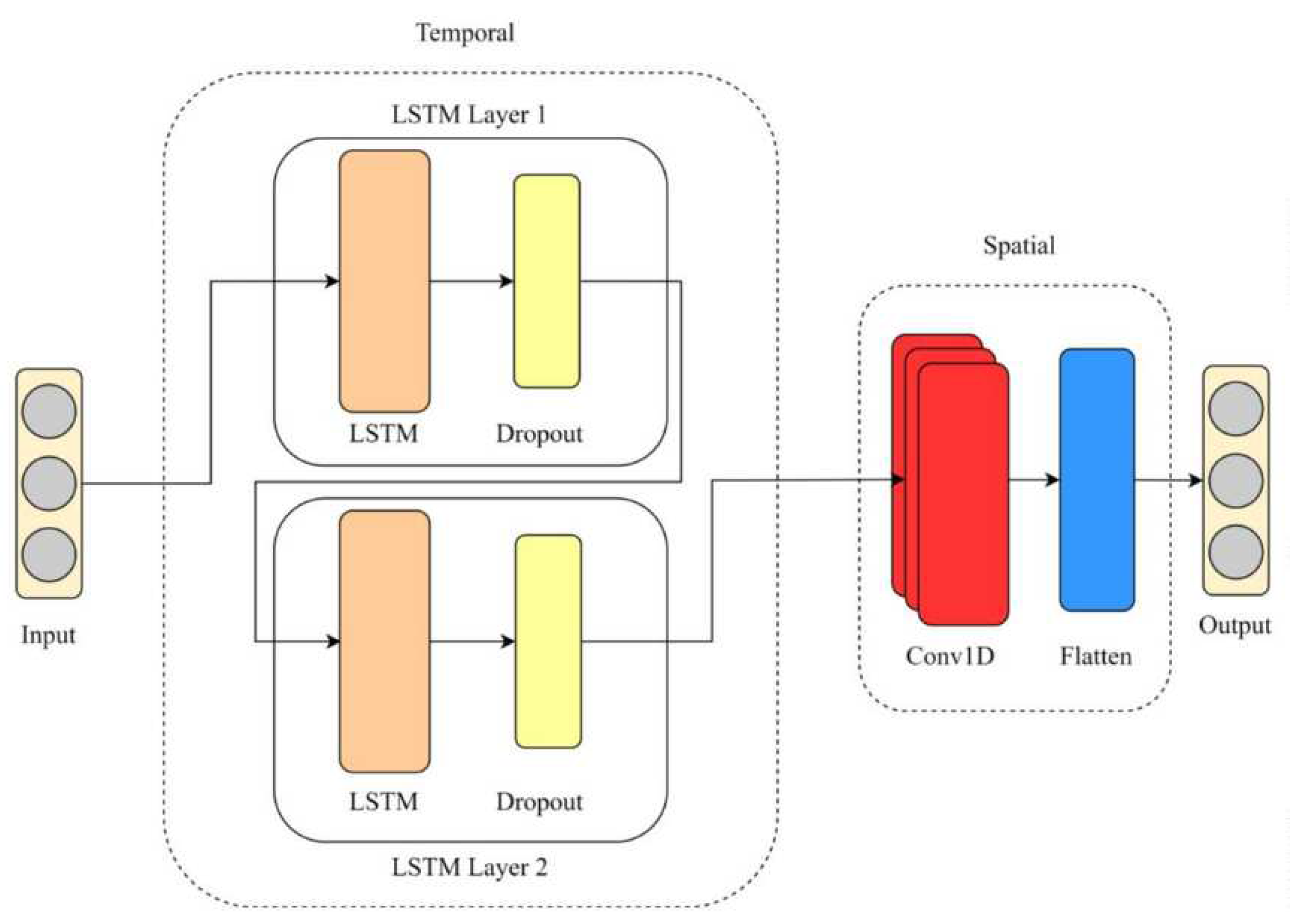
A graphical representation of the proposed recurrent neural network architecture and the sequential input-output data process is shown in
Figure 1.
Both neural networks have identical architectures, which include an Input layer, three LSTM layers with 32 units each, a Convolutional layer with 128 units, and a Dense layer with 48 neurons. The Dropout regularization method is applied to the LSTM layers with a value of 0.5. This method probabilistically excludes input connections from activation and weight updates during training, with the goal of reducing overfitting and enhancing model performance.
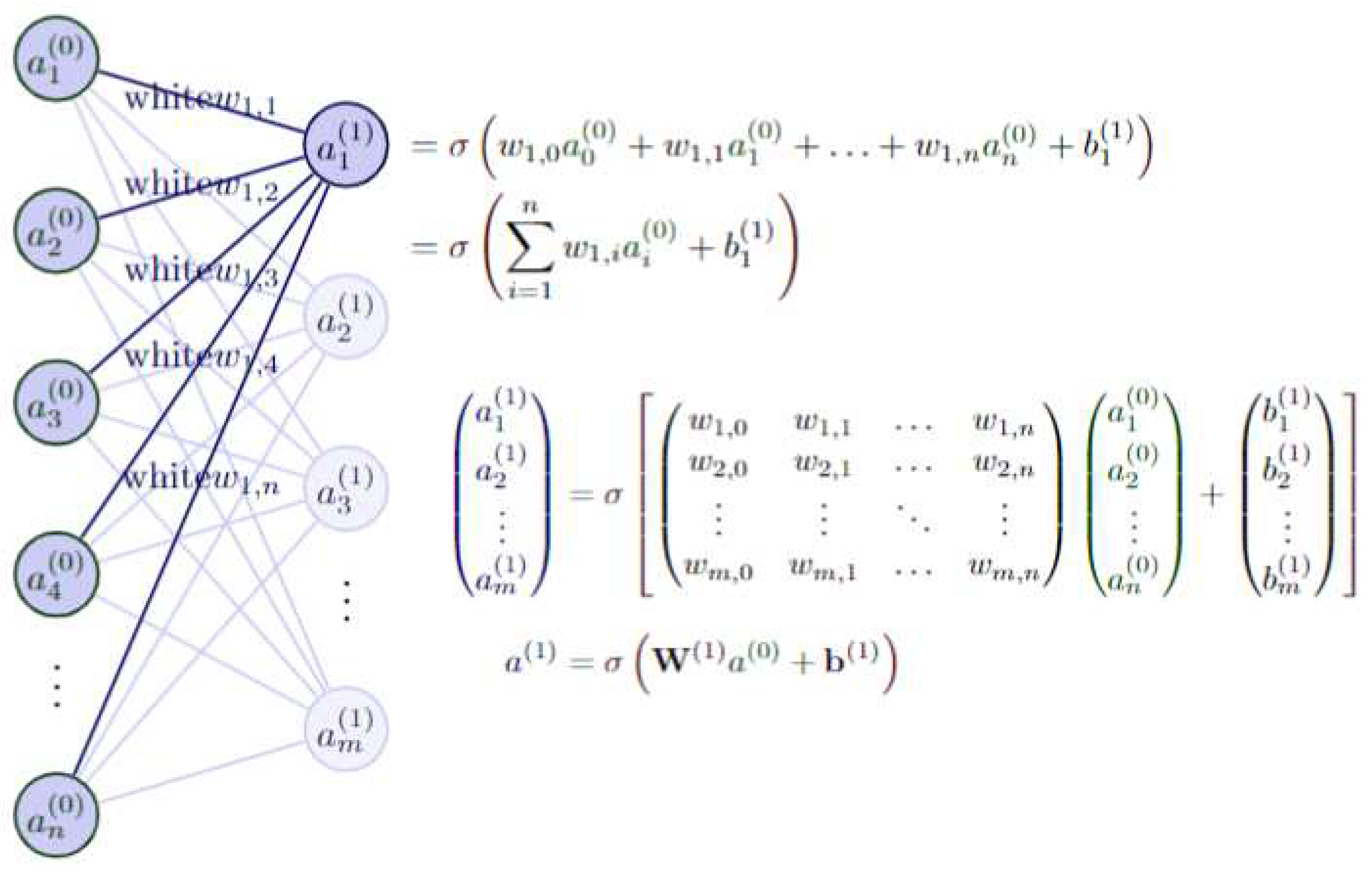
Figure 2 illustrates the final layer of the network, which is a Dense layer responsible for processing the information generated by the LSTM and Convolutional layers and producing the model's outputs. Each network forecast is calculated by applying the activation function, in this case, a linear activation function. This function operates on the sum of weights (w) and inputs (a), to which the bias (b) is added.
2.1. Hardware and experimental descriptions
The device developed for monitoring ventilation and thermal comfort, known as the 'AirQ-Monitor,' comprises the following fundamental hardware elements:
1x SoC ESP32 (integrated into the PCB): serves as the main system processor.
1x SCD30 sensor: a module for sensing the concentration of CO2, temperature, and humidity.
1x TFT 2.4" touch screen: used for equipment display and configuration interface.
Plastic chassis (derived from a generic model).
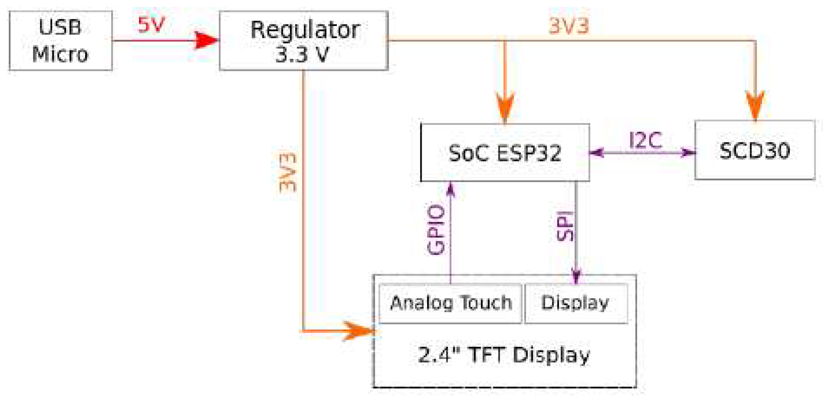
Figure 3 illustrates the system architecture, depicting multiple AirQ-Monitor devices connected to a server. The system is powered by a 5-volt source through a micro USB connector. Since all components operate at 3.3 volts, a voltage regulator is employed to reduce the voltage to this level. The ESP32 communicates with the SCD30 module through an I2C bus at a frequency of 100kHz. For controlling and displaying measurements on the screen, as well as handling other graphical elements, one of the SPI interfaces of the SoC is utilized. The touch panel, which enables user interaction with the device, operates in an analog manner and does not use any specific bus or standard protocol. Additionally, the collected data are transmitted to a cloud IoT server via a WiFi network.
Figure 3 provides a block diagram that visually represents the composition of the device.
Data processing has been performed using the TensorFlow framework. The data used to train the network was collected from devices installed on the campus of the Universitat Politècnica de Valencia in Spain. Data have been collected from various locations since March 2022. Eighty percent of the data was utilized for training the model, while the remaining 20% was used for evaluation.
2.2. Server and model deployment
As an additional aspect of this research, the proposed model has been implemented on a real-time server. The development of the real-time server processing utilized the 'Flask' framework. The server is hosted on a cloud computing machine and offers several accessible endpoints. Below, we describe some characteristics of these processes:
Results: Provides the most current forecast values.
Input: Displays the input values used to generate the most recent forecasts.
Real: Presents the forecasted values that correspond to the previous input, allowing for a comparison between the model's estimates and the actual values (from the last input)
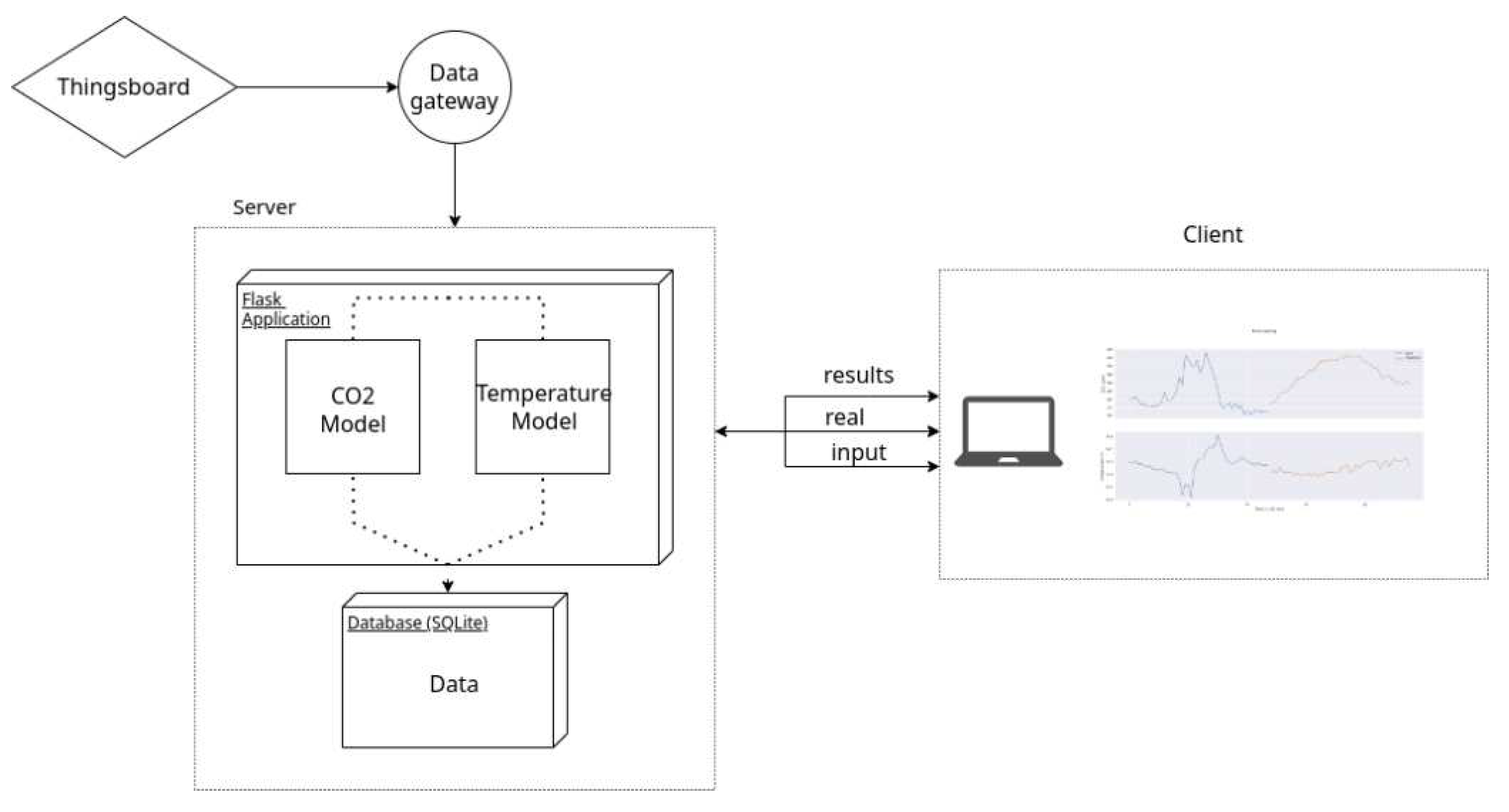
Figure 4 illustrates the system architecture after receiving data from the Thingsboard cloud, which was used in the experiment.
A Python-based data gateway handles the regular and automatic communication between the Thingsboard platform and the server. The server hosts the models for CO2 and temperature, which process incoming information and generate forecasts. Data related to the input, forecasts, and timestamps are stored in a SQLite database for future use. Clients can request information from the server through endpoints such as 'result,' 'real,' and 'input,' enabling the presentation of results in a suitable format for decision-making.
3. Results and discussion
For the implementation of the proposed model, a 48-step sliding window is used, which is equivalent to one day (24 hours). The data is sampled at a frequency of every 30 minutes, and the model generates forecasts with a horizon of 48 steps, also equivalent to one day with the same sampling frequency. The objective is to provide a reliable 24-hour forecast for both CO2 and temperature, based solely on their behavior in the preceding 24 hours.
Figure 5 and
Figure 6 display the results obtained during the model training process for the variables CO
2 and temperature, respectively.
As part of the analysis of CO
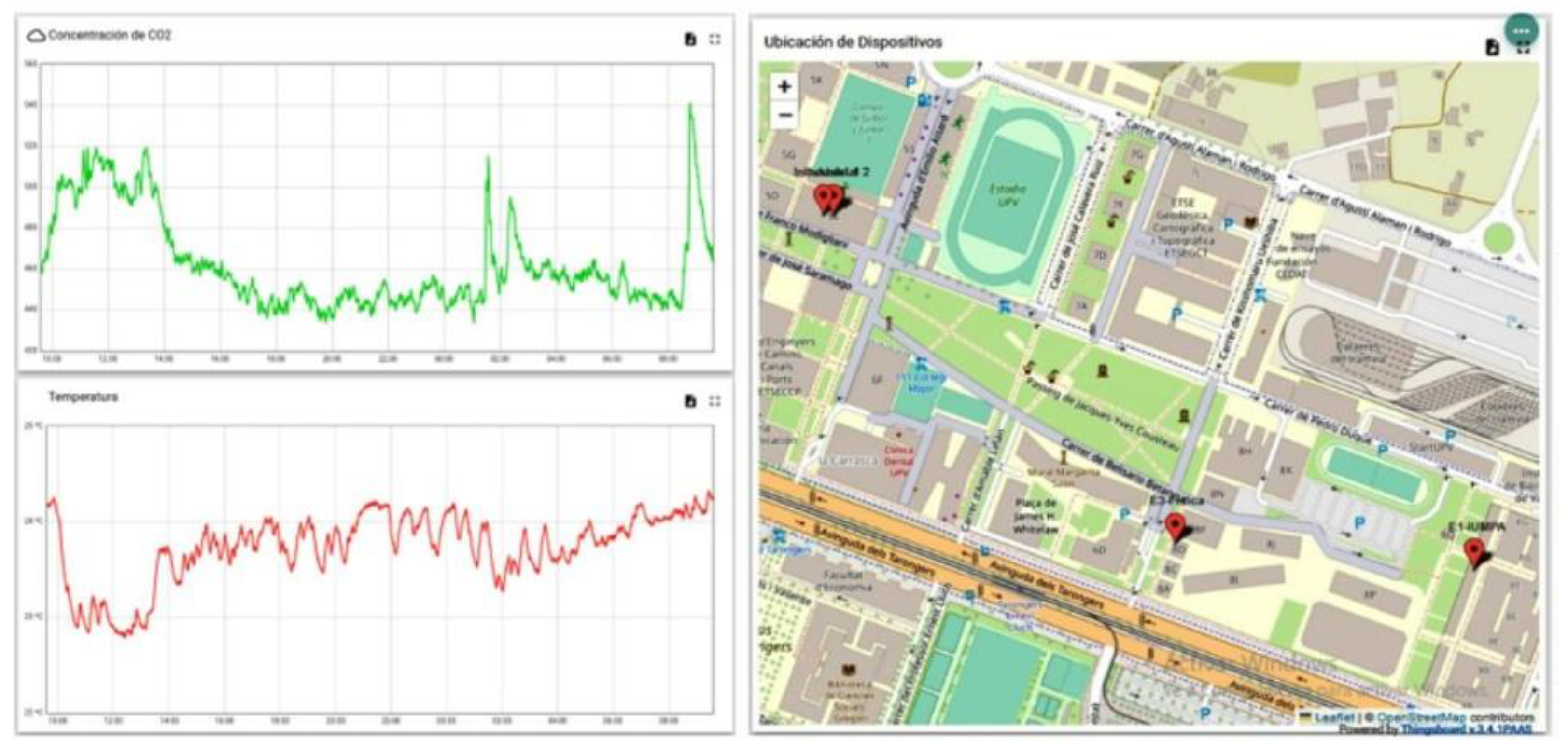
2 samples acquired by the developed device, we processed over 200.000 samples, each acquired at a 60-second interval. However, for the prediction task, the model operated with a 30-minute interval between samples, allowing us to evaluate its performance across various temporal horizons. The data for processing were acquired from the platform of the developed ventilation monitoring system, Thingsboard. In
Figure 7, you can observe a screenshot of the cloud visualization platform and the data obtained from the sensors.
Initially, the proposed model is trained using all the acquired data. The process of running the trained model unfolds as follows: Every 30 minutes, a dataset frame is automatically sent from the cloud (Thingsboard) to the server, updating the information related to the behavior of CO
2 and temperature during the previous 24 hours. Subsequently, the model predicts the behavior of CO
2 and temperature for the next 24 hours.
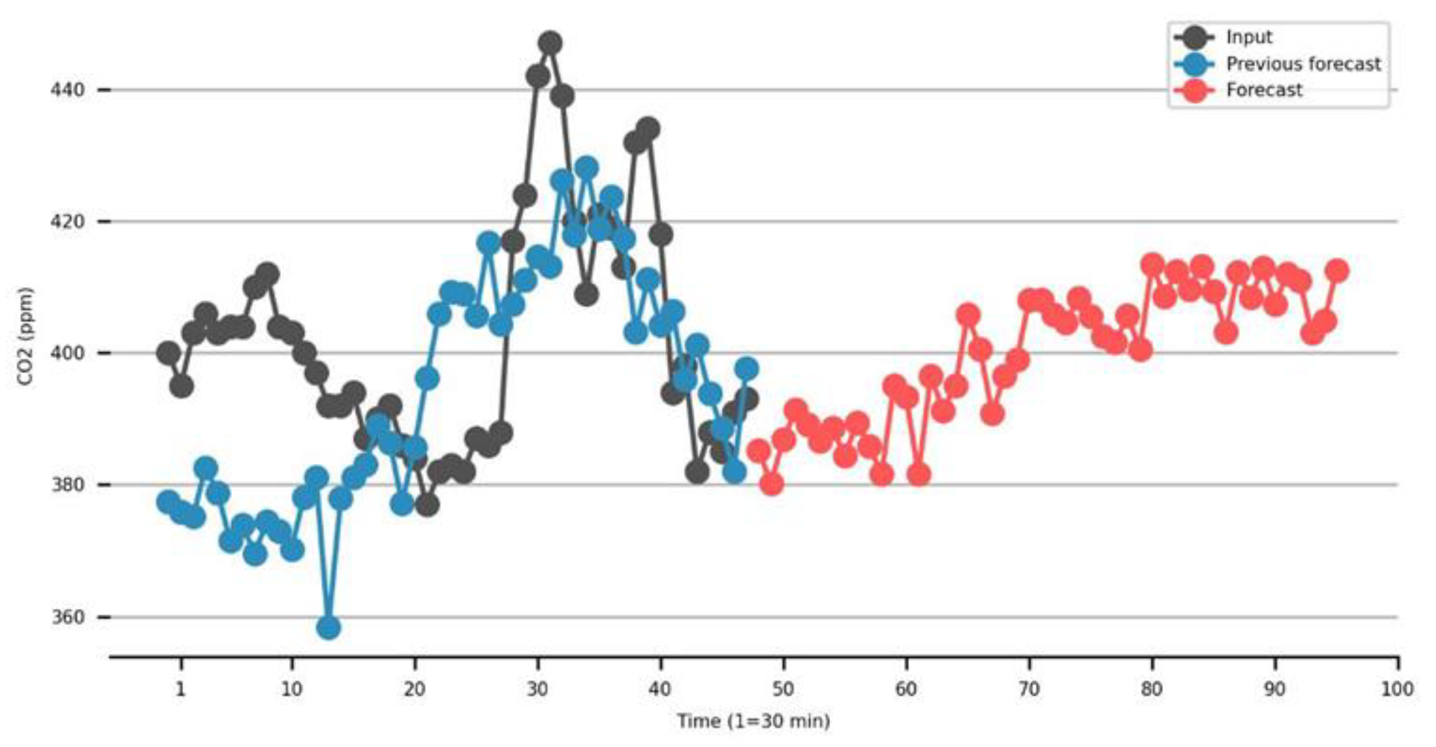
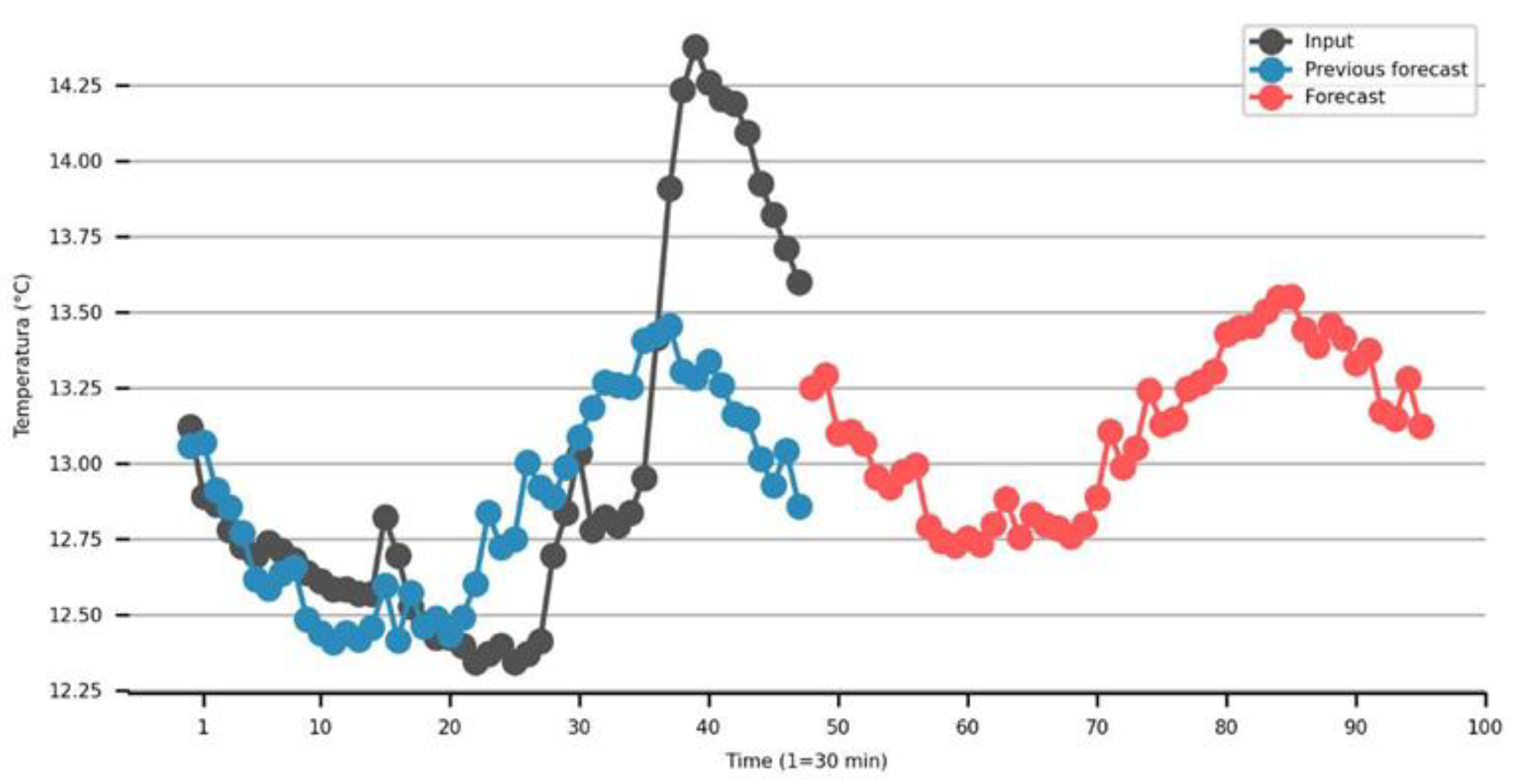
Figure 8 and
Figure 9, respectively, provide screenshots of the obtained results using a sliding window and a 24-hour temporal horizon. It's important to note that the results displayed in
Figure 8 and
Figure 9 are continuously updated as the server processes incoming samples. This process operates in real-time.
After evaluating the model, an error value of 13.8160 ppm was obtained for the 24-hour forecasts of CO2, and 0.4623 °C for temperature.
Additionally,
Table 1 displays the metrics obtained during the model's training evaluation. These metrics provide insights into the efficiency and accuracy of the proposed model for real-time prediction of environmental variables.
4. Discussion: Comparison with other methods
In order to verify the effectiveness of the proposed architecture in this work, we conduct a comparative analysis with other models from previous research. The comparison includes the following architectures: Long Short-Term Memory (LSTM), Convolutional Neural Network (CNN), Gated Recurrent Unit (GRU), and two hybrid variants of the LSTM and CNN architectures.
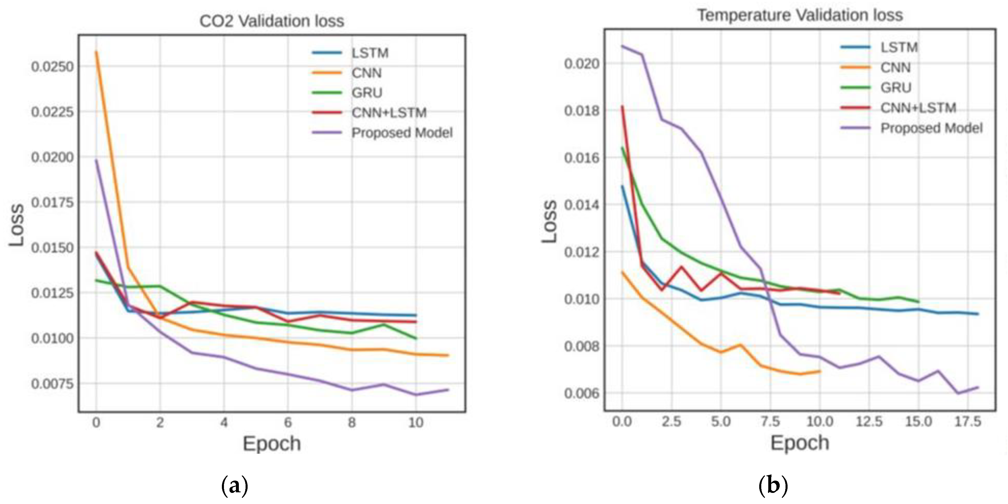
The models used for the comparative study were trained on the same Carbon Dioxide and Temperature data obtained from Universitat Politècnica de València. The Early-Stopping method is applied to prevent overfitting.
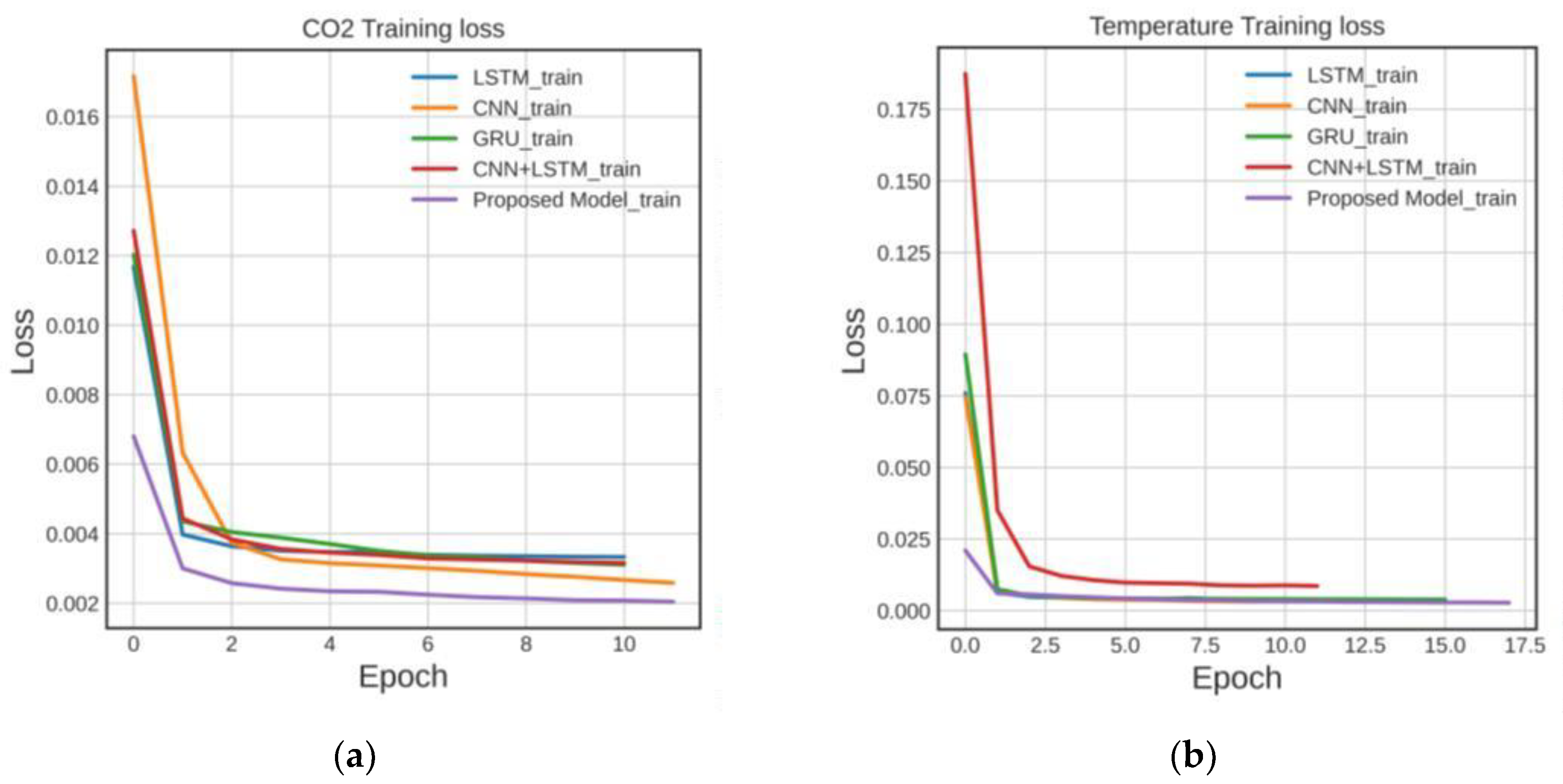
Figure 10 illustrates that for both the carbon dioxide and temperature models, the error minimization curve during training exhibits a shallower slope in the proposed model compared to the other evaluated architectures.
On the other hand, in
Figure 10, in terms of validation loss metrics, the proposed model demonstrates superior performance and lower errors. While temperature initially exhibits a high error and slower convergence, its error minimization is also more significant compared to other methods.
The results demonstrate that the architecture proposed in this work, utilizing a hybrid model with modifications in the pooling layer structure, yields superior CO
2 and temperature data forecasts.
Table 2 summarizes the obtained results in terms of validation losses, quantifying the total number of errors in the validation set.
5. Conclusions
This study has presented the outcomes of predictive analysis involving CO2 and temperature values using a novel hybrid neural network architecture. The developed predictive model for high-frequency time series aims to assess the behavior of these variables and their potential impact on indoor spaces' occupant performance when ventilation levels are insufficient. The novelty of our model lies in its omission of the pooling layer to prevent information loss within the network. Notably, we achieved favorable results up to 48 time steps into the future with a 30-minute sampling interval.
Our model operates in real-time by synchronizing with a cloud-based data server, ensuring continuous learning and enhancing forecasting performance. Furthermore, the proposed architecture offers optimization flexibility concerning data window size and the prediction time horizon. These findings highlight the model's potential for improving indoor air quality and supporting decision-making for maintaining optimal environmental conditions.
Author Contributions
Conceptualization, M.E.I.M and P.F.C.; methodology, J.G.C and F.G.P; software, C.A.R.P and E.B.; validation, C.A.R.P., M.E.I.M and P.F.C; formal analysis, H.M.A and M.E.I.M; investigation, C.A.R.P, E.B.; resources, F.G.P., H.M.A. and M.E.I.M; data curation, F.G.P., E.B. and J.G.C; writing—original draft preparation, C.A.R.P; writing—review and editing, H.M.A, M.E.I.M and P.F.C.; visualization, J.G.C.; supervision, F.G.P. and P.F.C. All authors have read and agreed to the published version of the manuscript.
Funding
This research received no external funding.
Data Availability Statement
Not applicable.
Acknowledgments
Miguel E. Iglesias Martínez's research was supported by a postdoctoral research scholarship titled 'Ayudas para la Recualificación del Sistema Universitario Español 2021-2023, Modalidad: Margarita Salas,' funded by the UPV, Ministerio de Universidades, Plan de Recuperación, Transformación y Resiliencia, Spain, and made possible by the European Union-Next Generation EU. The authors would like to express their gratitude for the invaluable support and facilities provided by the Galician Supercomputing Center (CESGA:
https://www.cesga.es/) for conducting modeling calculations.
Conflicts of Interest
The authors declare no conflict of interest.
References
- W.Michael Alberts. Indoor air pollution: NO, NO2, CO, and CO2. Journal of Allergy and Clinical Immunology,94(2, Part 2):289-295, 1994. Building- and Home-Related Complaints and Illnesses: Sick Building Syndrome.
- Parajuli I, Lee H, Shrestha KR. Indoor air quality and ventilation assessment of rural mountainous households of Nepal. Int J Sustain Built Environ. 2016; 5:301–11. [CrossRef]
- Central Pollution Control Board & ASEM - GTZ. Conceptual Guidelines and Common Methodology for Air Quality Monitoring, Emission Inventory & Source Apportionment Studies for Indian Cities. Parivesh Bhawan, East Arjun Nagar, Delhi - 110 032. Draft, 2006.
- Stuart Batterman. Review and extension of CO2-based methods to determine ventilation rates with application to school classrooms. International journal of environmental research and public health, 14(2):145, 2017.
- Usha Satish, Mark J. Mendell, Krishnamurthy Shekhar, Toshifumi Hotchi, Douglas Sullivan, Siegfried Streufert, and William J. Fisk. Is CO2 an indoor pollutant? direct effects of low-to-moderate CO2 concentrations on human decision-making performance. Environmental Health Perspectives, 120(12):1671-1677, 2012.
- Medidores de CO2 de alta precisión con conexión a internet. Control de calidad del aire.
- SN Rudnick and DK Milton. Risk of indoor airborne infection transmission estimated from carbon dioxide concentration. Indoor air, 13(3):237-245, 2003.
- Wang, J.; Spicher, N.; Warnecke, J.M.; Haghi, M.; Schwartze, J.; Deserno, T.M. Unobtrusive Health Monitoring in Private Spaces: The Smart Home. Sensors 2021, 21, 864. [CrossRef]
- Franco, A.; Schito, E. Definition of Optimal Ventilation Rates for Balancing Comfort and Energy Use in Indoor Spaces Using CO2 Concentration Data. Buildings 2020, 10, 135. [CrossRef]
- Paula Matos, Joana Vieira, Bernardo Rocha, Cristina Branquinho, Pedro Pinho, Modeling the provision of air-quality regulation ecosystem service provided by urban green spaces using lichens as ecological indicators, Science of The Total Environment, Volume 665, 2019, Pages 521-530, ISSN 0048-9697, . [CrossRef]
- Ministry for the Environment. Good-Practice Guide for Air Quality Monitoring and Data Management. Prepared and published by the Ministry for the Environment, Wellington, New Zealand, PO Box 10 362. December 2000.
- Cincinelli A, Martellini T. Indoor air quality and health. Int J Environ Res Pu. 2017; 14:1286.
- Kim, T. & Kim, H. Y. Forecasting stock prices with a feature fusion LSTM-CNN model using different representations of the same data. PLoS ONE 14, e0212320 (2019).
- Zaytar, M. A. & El Amrani, C. Sequence to sequence weather forecasting with long short-term memory recurrent neural networks. Int. J. Comput. Appl. 143, 7– 11 (2016).
- Jain, A. K., Mao, J. & Mohiuddin, K. M. Artificial neural networks: A tutorial. Computer 29, 31-44 (1996).
- Papadatou-Pastou, M. Are connectionist models neurally plausible? A critical appraisal. Encephalos 48, 5–12 (2011).
- Huang, C.-J. & Kuo, P.-H. A deep CNN-LSTM model for particulate matter (PM25) forecasting in smart cities. Sensors 18, 2220 (2018).
- Hu, C. et al. Deep learning with a long short-term memory networks approach for rainfall-runoff simulation. Water 10, 1543 (2018).
- Liu, Y. et al. A long short-term memory-based model for greenhouse climate prediction. Int. J. Intell. Syst. 37(1), 135–151. (2022). [CrossRef]
- Liu,[Y.et](http://y.et/) al. An attention-based category-aware GRU model for the next POI recommendation. Int. J. Intell. Syst. 36(7), 1–16. (2021). [CrossRef]
- Liu, Y., Song, Z., Xu, X., Rafique, W., Zhang, X., & Shen, Z., et al. Bidirectional GRU networks- based next POI category prediction for healthcare. Int. J. Intell. Syst. (2021).
- Qing, X. & Niu, Y. Hourly day-ahead solar irradiance prediction using weather forecasts by LSTM. Energy 148, 461–468. (2018). [CrossRef]
- Karevan, Z.&Suykens, J.A.K. Transductive LSTM for time-series prediction: An application to weather forecasting. Neural Netw. 125, 1–9. (2020). [CrossRef]
- Salman, A. G., Heryadi, Y., Abdurahman, E. & Suparta, W. Single Layer and multi-layer long short-term memory (LSTM) model with intermediate variables for weather forecasting. Proc. Comput. Sci. 135, 89–98. (2018). [CrossRef]
- Azzouni, A., & Pujolle, G. A long short-term memory recurrent neural network framework for network traffic matrix prediction. ArXiv Preprint ArXiv:170505690 2017.
- Hochreiter, Sepp; Schmidhuber, Juergen (1996). LSTM can solve hard long time lag problems. Advances in Neural Information Processing Systems.
- Felix A. Gers; Ju¨rgen Schmidhuber; Fred Cummins (2000). Learning to Forget: Continual Prediction with LSTM. Neural Computation. 12 (10): 2451- 2471. CiteSeerX 10.1.1.55.5709. PMID 1103 2042. S2CID 11598600. [CrossRef]
- Khan, S., Rahmani, H. & Shah, S. A guide to convolutional neural networks for computer vision. Synth. Lect. Comput. Vis. 8, 1–207 (2018).
- Qin, J., Pan, W. & Xiang, X. A biological image classification method based on improved CNN. Ecol. Inform. (2020). [CrossRef]
- Nasir, J. A., Khan, O. S. & Varlamis, I. Fake news detection: A hybrid CNN-RNN based deep learning approach. Int. J. Inf. Manag. Data Insights. 1, 100007 (2021).
- Qiao, Y., Wang, Y., Ma, C. & Yang, J. Short-term traffic flow prediction based on 1DCNN-LSTM neural network structure. Mod. Phys. Lett. B 35, 2150042 (2020).
- Cheng, J., Liu, Y. & Ma, Y. Protein secondary structure prediction based on integration of CNN and LSTM model. J. Vis. Commun. Image Represent. 71, 102844 (2020).
- Pei Li, Mohamed Abdel-Aty, Jinghui Yuan, Real-time crash risk prediction on arterials based on LSTM-CNN, Accident Analysis & Prevention, Volume 135, 2020, 105371, ISSN 0001-4575, . [CrossRef]
- Tae-Young Kim, Sung-Bae Cho, predicting residential energy consumption using CNN-LSTM neural networks, Energy, Volume 182, 2019, Pages 72-81, ISSN 0360-5442, . [CrossRef]
- Livieris, I.E., Pintelas, E. & Pintelas, P. A CNN–LSTM model for gold price time-series forecasting. Neural Comput & Applic 32, 17351–17360 (2020). [CrossRef]
- Md. Omer Faruque, Md. Afser Jani Rabby, Md. Alamgir Hossain, Md. Rashidul Islam, Md Mamun Ur Rashid, S.M. Muyeen. A comparative analysis to forecast carbon dioxide emissions, Energy Reports, Volume 8, 2022, Pages 8046-8060, ISSN 2352-4847, . [CrossRef]
|
Disclaimer/Publisher’s Note: The statements, opinions and data contained in all publications are solely those of the individual author(s) and contributor(s) and not of MDPI and/or the editor(s). MDPI and/or the editor(s) disclaim responsibility for any injury to people or property resulting from any ideas, methods, instructions or products referred to in the content. |
© 2023 by the authors. Licensee MDPI, Basel, Switzerland. This article is an open access article distributed under the terms and conditions of the Creative Commons Attribution (CC BY) license (http://creativecommons.org/licenses/by/4.0/).
