Phase Transition in Ant Colony Optimization

Preprint

Article

Phase Transition in Ant Colony Optimization

Altmetrics

Downloads

Views

Comments

A peer-reviewed article of this preprint also exists.

Shintaro Mori^*,Shogo Nakamura,Kazuaki Nakayama,Masato Hisakado

This version is not peer-reviewed

Submitted:

17 October 2023

Posted:

19 October 2023

You are already at the latest version

Alerts

Abstract

Ant Colony Optimization (ACO) is a stochastic optimization algorithm inspired by the foraging behavior of ants. We investigate a simplified computational model of ACO, wherein ants sequentially engage in binary decision-making tasks, leaving pheromone trails contingent upon their choices. The quantity of pheromone left is the number of correct answers. We scrutinize the impact of a salient parameter in the ACO algorithm, specifically, the exponent $\alpha$ that governs the pheromone levels in the stochastic choice function. In the absence of pheromone evaporation, the system is accurately modeled as a multivariate nonlinear P\'{o}lya urn, undergoing a phase transition as $\alpha$ varies. The probability of selecting the correct answer for each question asymptotically approaches the stable fixed point of the nonlinear P\'{o}lya urn. The system exhibits dual stable fixed points for $\alpha\ge \alpha_c$ and a singular stable fixed point for $\alpha<\alpha_c$. When pheromone evaporates over a time scale $\tau$, the phase transition does not occur and leads to a bimodal stationary distribution of probabilities for $\alpha\ge \alpha_c$ and a monomodal distribution for $\alpha<\alpha_c$.

Keywords:

Subject: Physical Sciences - Theoretical Physics

0. Introduction

"Socio-physics emerged in the 1970s and has evolved into a captivating research field within statistical physics [1,2]. In particular, herding behavior, or the inclination to follow the majority, has captured the attention of many researchers due to its pivotal role in understanding social phenomena [3,4,5,6,7,8]. Various probabilistic models have been proposed to describe herding behavior, with one notable example being the ant recruitment model. This model explains the intermittent oscillation observed in ants when they are presented with two identical food sources [9,10]. When ants choose a food source among two food sources, it incorporates a straightforward herding mechanism in which a randomly selected ant chooses one of the two based on the number of ants that have already made the same choice. Scouts play a crucial role by exploring the terrain to locate food sources [11,12]. When a scout discovers food, it returns to the nest, leaving a pheromone trail in its wake. Other ants are drawn to these pheromone marks and consequently become recruited to forage at the food source."

Ant Colony Optimization (ACO) is a model-based meta-heuristic inspired by the foraging behavior of ants in their search for the shortest path to food sources [13,14,15]. While ants may not be highly intelligent individually, they collectively find the shortest path by following pheromone trails left by their fellow ants. The optimal path is determined by the route on which the maximum number of ants travel[12]. Consider a classic problem known as the traveling salesman problem (TSP), which involves finding the shortest possible route that visits each city in a given list exactly once and returns to the origin city. In ACO, ants make decisions about their next city to visit based on a concept called ’pheromone.’ Pheromone represents the preference for a particular choice and is collaboratively learned by the ants during their search process [16]. In the context of TSP, pheromone values are typically associated with pairs of cities and reflect the preference for traveling from one city to another within the pair. These pheromone values are learned through a reinforcement strategy, where each ant reinforces its chosen paths based on the quality of the solution constructed. This quality is often determined by the inverse of the total length of the route. ACO has found successful applications in various industrial and academic constraint optimization problems and has become one of the most popular methods.

ACO has seen significant improvements, and modern ACO algorithms deviate substantially from the original ACO[17]. The fundamental modification lies in controlling the diversity of solutions and achieving convergence [18,19]. In this context, ’convergence’ refers to the tendency of ants to cluster around similar solutions in the neighborhood and ultimately converge toward the same solution. Early convergence to a small region of the search space leaves large sections of the search space unexplored and fails to find good solutions. On the other hand, very slow convergence means that the computational cost required to reach good solutions is high, rendering the search inefficient. Diversity control aims to prevent complete convergence by slowing down the search process.

Many algorithms have been proposed for controlling the diversity of the ACO algorithm. One of the diversity control mechanisms involves modifying the probabilistic decision function [17,20]. Meyer studied the influence of

α

, the exponent on the pheromone level in the selection function, and suggested that

α

qualitatively determines diversity and convergence behavior. Additionally, he introduced a dynamic

α

that changes throughout the search process to enhance search efficiency, a technique known as

α

-"annealing". In this paper, we study a simple model of ACO in which ants sequentially answer a series of two-choice quizzes. We investigate the phase transition and the qualitative change of the convergence behavior by varying

α

. In Section 1, we introduce a model and derive stochastic differential equations (SDEs) using the diffusion approximation. In Section 2, we investigate the time evolution and examine the effect of

α

on the convergence properties of the solutions. Section 3 provides a summary of the results. Appendix A explains the estimation of the initial conditions for the SDEs.

1. Materials and Methods

There are N two-choice quizzes, each of which is answered by a large number of ants sequentially[21]. These quizzes are labeled by

n = 1, \dots, N

. The answer provided by the t-th ant is denoted as

X (n, t) \in {0, 1}

, where

X (n, t) = 1

indicates a correct answer, and

X (n, t) = 0

indicates an incorrect answer. Each ant receives 1 point for a correct answer. After ant t has answered all N questions, the total points (TP) earned by the ant can be calculated using the following equation,

TP (t) = \sum_{n = 1}^{N} X (n, t) .

Ant t deposits pheromones on his answer

X (n, t) \in {0, 1}

. The amount of the pheromones is

TP (t)

. We assume that the pheromones evaporate and decrease by

e^{- 1 / τ}

per unit time. Here

τ

represents the time scale of the pheromone evaporation.

Ant

t + 1

observes the total values of the pheromones associated with question m for each choice

X (m, t + 1) = {0, 1}

. We denote the total value of pheromones that remains on all the questions after ant t has answered,

S (t) \equiv \sum_{s = 1}^{t} TP (s) e^{t - s} = \sum_{s = 1}^{t} \sum_{n = 1}^{N} X (n, s) e^{t - s} .

(1)

Then, the remaining pheromone on

X (m, s) = 1, 1 \leq s \leq t

is,

S (m, t) \equiv \sum_{s = 1}^{t} TP (s) X (m, s) e^{t - s} = \sum_{s = 1}^{t} \sum_{n = 1}^{N} X (n, s) X (m, s) e^{t - s} .

(2)

The remaining pheromone on

X (m, s) = 0, 1 \leq s \leq t

is given by

S (t) - S (m, t)

Ants are not highly intelligent, and the probability of them making the correct choice in the two-choice quizzes by themselves is 1/2. The information provided by

T P (s)

gives them an indirect clue about the correct choice. If TP

(s) > N / 2

, the posterior probability for

X (m, s) = 1

is larger than

1 / 2

. Similarly, if

S (m, t)

is greater than

S (t) / 2

, the posterior probability for

X (m, t + 1) = 1

is greater than

1 / 2

. In ACO, a decision function is introduced that uses the values of the pheromones as follows,

P (X (m, t + 1) = 1) = (1 - ϵ) \frac{S {(m, t)}^{α}}{S {(m, t)}^{α} + {(S (t) - S (m, t))}^{α}} + \frac{1}{2} ϵ .

(3)

Here, the exponent

α

determines the response of the choice to the values of the pheromones.

ϵ > 0

is a small positive constant to avoid the absorbing states

S (m, t) = 0

and

S (m, t) = S (t)

of the stochastic process.

We denote the ratio of the remaining pheromones on the correct choices as

Z (m, t)

Z (m, t) \equiv \frac{S (m, t)}{S (t)} .

We divide both the denominator and numerator of eq.(3) by

S {(t)}^{α}

, and the probability of the correct choice

X (m, t + 1) = 1

is expressed as,

P (X (m, t + 1) = 1) = (1 - ϵ) (\frac{Z {(m, t)}^{α}}{Z {(m, t)}^{α} + {(1 - Z (m, t))}^{α}}) + \frac{1}{2} ϵ = f (Z (m, t)) .

Here,

f (z)

is defined as

f (z) \equiv (1 - ϵ) (\frac{z^{α}}{z^{α} + {(1 - z)}^{α}}) + \frac{1}{2} ϵ .

(4)

We note that

f (1 / 2) = 1 / 2

and

f (1 - x) = 1 - f (x)

. The slope of

f (x)

x = 1 / 2

(1 - ϵ) α

. We also introduce the discount factor

D (t)

and the ratio of correct answers

Z (t)

as,

\begin{matrix} D (t) & = & \sum_{n = 1}^{N} \sum_{s = 1}^{t} e^{- (t - s) / τ} = N (\frac{1 - e^{- t / τ}}{1 - e^{- 1 / τ}}) \\ Z (t) & = & \frac{S (t)}{D (t)} . \end{matrix}

1.1. Stochastic Differential equation

First, we derive the recursive relation for

S (t)

and

D (t)

. According to the definition,

D (t + 1)

and

S (t + 1)

obey the next recursive relations,

\begin{matrix} D (t + 1) & = & N + D (t) e^{- 1 / τ} \\ S (t + 1) & = & \sum_{i = 1}^{N} X (i, t + 1) + S (t) e^{- 1 / τ} . \end{matrix}

τ

is finite, for

t > > τ > > 1

, we have

D (t) ≃ N τ

. In the limit

τ \to \infty

, the pheromone does not evaporate, and we have

D (t) = N t

For

N > > 1

, we can replace the sum of

X (i, s), i = 1, \dots, N

with the sum of the expected values using the law of large numbers. We obtain,

S (t + 1) ≃ \sum_{i = 1}^{N} f (Z (i, t)) + S (t) e^{- 1 / τ} .

We denote the average of

f (Z (i, t))

\bar{f (Z (i, t))}

\bar{f (Z (i, t))} \equiv \frac{1}{N} \sum_{i = 1}^{N} f (Z (i, t)) .

We have

S (t + 1) ≃ S (t) e^{- 1 / τ} + N \bar{f (Z (i, t))} .

The recursive relation for

Z (t)

Z (t + 1) ≃ \frac{S (t + 1)}{D (t + 1)} = \frac{D (t + 1) - N}{D (t + 1)} \cdot Z (t) + \frac{N}{D (t + 1)} \cdot \bar{f (Z (i, t)}

Δ Z (t) \equiv Z (t + 1) - Z (t)

is given as,

Δ Z (t) ≃ \frac{N}{D (t + 1)} (\bar{f (Z (i, t))} - Z (t)) .

In the continuous time limit

d t = 1 \to 0

, we obtain

\frac{d}{d t} Z (t) = \frac{N}{D (t + 1)} (\bar{f (Z (i, t))} - Z (t)) .

(5)

One see that

Z (t)

converges to

\bar{f (Z (i, t))}

. However, when the pheromones evaporate and

τ < \infty

D (t) ≃ N τ

and the prefactor of the differential equation is

1 / τ

. If one assume that the dynamics of

Z (i, t)

is faster than that of

Z (t)

(adiabatic approximation), the time scale of the convergence is given by

τ

\bar{f (Z (i, t))} - Z (t) \propto e^{- t / τ}

. When the pheromone does not evaporate and

τ \to \infty

D (t) ≃ N t

. The prefactor of the differential equation is

1 / t

, and

\bar{f (Z (i, t))} - Z (t) \propto t^{- 1}

. The convergence becomes extremely slow.

Next, we study the dynamics of

Z (m, t)

. The recursive relation for

S (m, t)

is,

S (m, t + 1) = S (m, t) e^{- 1 / τ} + X (m, t + 1) (\sum_{i = 1 \neq m}^{N} X (i, t + 1) + 1) .

Z (m, t + 1)

is then estimated as,

\begin{matrix} Z (m, t + 1) & = & \frac{S (m, t + 1)}{S (t + 1)} = \frac{S (t) e^{- 1 / τ}}{S (t + 1)} \cdot Z (m, t) + \frac{\sum_{i \neq m} X (i, t + 1) + 1}{S (t + 1)} \cdot X (m, t + 1) \\ ≃ & \frac{S (t + 1) - N \bar{f (Z (i, t))}}{S (t + 1)} \cdot Z (m, t) + \frac{N \bar{f (Z (i, t))} + (1 - f (Z (m, t))}{S (t + 1)} \cdot X (m, t + 1) . \end{matrix}

Using

S (t + 1) = D (t + 1) Z (t + 1)

, we obtain

Δ Z (m, t) = \frac{N \bar{f (Z (i, t))}}{D (t + 1) Z (t + 1)} ((1 + \frac{(1 - f (Z (m, t)))}{N \bar{f (Z (i, t))}}) X (m, t + 1) - Z (m, t)) .

We denote the history of

Z (s), {Z (i, s)}_{i = 1, \dots, N}, s = 1, \dots, t

H_{t}

, and the conditional expected value of

Δ Z (m, t)

is estimated as

E (Δ Z (m, t) | H_{t}) = \frac{N \bar{f (Z (i, t))}}{D (t + 1) Z (t + 1)} ((1 + \frac{(1 - f (Z (m, t)))}{N \bar{f (Z (i, t))}}) f (Z (m, t)) - Z (m, t)) .

(6)

Likewise, the conditional variance of

Δ Z (m, t)

can be approximated as,

V (Δ Z (m, t) | H_{t}) ≃ {(\frac{N \bar{f (Z (i, t)}}{D (t + 1) Z (t + 1)})}^{2} f (Z (m, t)) (1 - f (Z (m, t))) .

Here, we neglect the subleading terms in

{(1 + \frac{(1 - f (Z (m, t)))}{N \bar{f (Z (i, t))}})}^{2}

. We read the drift and diffusion term from the results and the SDEs are,

d Z (m, t) = E (Δ Z (m, t) | H_{t}) d t + \sqrt{V (Δ Z (m, t) | H_{t})} d W (t), m = 1, \dots, N .

(7)

Here,

W (t)

is the Wiener process. Eq.(5) and eq.(7) describe the dynamics of the system. The system can be described as a multi-variate Pólya urn process.

We note that

\frac{(1 - f (Z (m, t)))}{N \bar{f (Z (i, t))}}

in eq.(6) breaks the

Z_{2}

symmetry of the system. If one neglects the term,

E (Δ Z (m, t) | H_{t})

is proportional to

f (Z (m, t)) - Z (m, t)

. As

f (1 - x) = 1 - f (x)

f (1 - x) - (1 - x) = - (f (x) - x)

holds.

Z (m, t)

and

1 - Z (m, t)

obeys the same dynamics and we call the symmetry

Z_{2}

symmetry. The term is always positive and drives

Z (m, t)

in the positive direction. As the term is proportional to

1 / N

, the strength of the

Z_{2}

-symmetry breaking field becomes smaller as N becomes larger.

2. Results

We analyze the SDEs given in eq.(7) and investigate the convergence properties of

Z (m, t)

. As the convergence behavior relies on the initial value of

Z (m, t = t_{0})

in the context of the non-linear Pólya urn model, we commence by examining the distribution of

Z (m, t)

2.1. Initial distribution of ${Z (m, t)}$

We assume that ants adopt

α = 0

and do not respond to the values of the pheromones for

t = 1, \dots, t_{0}

. The ants answer the questions independently and

P (X (i, t) = 1) = 1 / 2

. We estimate

Z (t)

and

Z (m, t)

for

τ < t \leq t_{0}

as follows.

\begin{matrix} Z (t) & \sim & N (\frac{1}{2}, \frac{D_{h} (t)}{4 D {(t)}^{2}}), \\ Z (m, t) & \sim & N (\frac{1}{2} + \frac{1}{2 N}, \frac{N D_{h} (t)}{4 D {(t)}^{2}}), \\ D_{h} (t) & \equiv & N \sum_{s = 1}^{t} e^{- 2 (t - s) / τ} = N \cdot \frac{1 - e^{- 2 t / τ}}{1 - e^{- 2 / τ}} . \end{matrix}

(8)

The details of the calculations are given in Appendix A. If

τ

is finite, we have

D_{h} (t) ≃ N τ / 2

for

t > > τ > > 1

. In the limit

τ \to \infty

, the pheromone does not evaporate and we have

D_{h} (t) = N t

The essential differences between

Z (t)

and

Z (m, t)

include a shift of the expected value by

1 / 2 N

and the presence of a factor of N in the numerator of the variance of

Z (m, t)

. The shift of

1 / 2 N

arises from the fact that

X (m, s)

S (m, t)

is 1, which is larger than

E [X (i, s)] = 1 / 2

for

i \neq m

. The value of the pheromone contains information about the correct choice, leading to

E [S (m, t)] > \frac{1}{2} E [S (t)]

. However, in the "cheating" process, the variables

X (i, s), i = 1, \dots, N

are combined by

X (m, s)

as in eq.(2), resulting in a larger variance for

S (m, t)

. The factor of N in the numerator of the variance of

Z (m, t)

is a consequence of this combination process.

From the distribution of

Z (m, t_{0})

, one can determine the values of

τ

t_{0}

that guarantee that

Z (m, t_{0})

is greater than 0.5 for the limits

t > > τ > > 1

and

τ \to \infty

, respectively. With a confidence level of 1%,

τ

and

t_{0}

should satisfy the following conditions:

\begin{matrix} t > > τ > > 1 : \frac{1}{2 N} \geq \frac{2.58}{2 \sqrt{2} τ} \to τ \geq 3.33 N^{2} \\ τ \to \infty : \frac{1}{2 N} \geq \frac{2.58}{2 \sqrt{t_{0}}} \to t_{0} \geq 6.66 N^{2} . \end{matrix}

2.2. $τ \to \infty$ case

We take the limit

τ \to \infty

in eq.(5) and eq.(7). We replace

D (t + 1)

and

D_{h} (t + 1)

with

N (t + 1)

and

N (t + 1)

, respectively. This results in the following equations:

\begin{matrix} d Z (m, t) & = & \frac{\bar{f (Z (i, t))}}{(t + 1) Z (t + 1)} ((1 + \frac{(1 - f (Z (m, t)))}{N \bar{f (Z (i, t))}}) f (Z (m, t)) - Z (m, t)) d t \\ + & (\frac{\bar{f (Z (i, t))}}{(t + 1) Z (t + 1)}) \sqrt{f (Z (m, t) (1 - f (Z (m, t)))} d W (t), m = 1, \dots, N \\ \frac{d}{d t} Z (t) & = & \frac{1}{(t + 1)} (\bar{f (Z (i, t))} - Z (t)) . \end{matrix}

The initial conditions of

Z (t)

and

Z (m, t)

t = t_{0}

are as follows:

\begin{matrix} Z (t_{0}) & \sim & N (\frac{1}{2}, \frac{1}{4 N t_{0}}), \\ Z (m, t_{0}) & \sim & N (\frac{1}{2} + \frac{1}{2 N}, \frac{1}{4 t_{0}}) . \end{matrix}

In the adiabatic approximation, where the time development of

Z (m, t)

is much faster than that of

Z (t)

, the structure of the SDE for each

Z (m, t)

, where

m = 1, \dots, N

, is the same as that of a non-linear P’olya urn [22,23]. The probability for

Z (m, t)

to converge to a stable solution of the following equation is positive[24].

(1 + \frac{(1 - f (z))}{N \bar{f (Z (i, t))}}) f (z) = z .

(9)

Here, a stable (unstable) solution of eq.(9) means that the curve of the left-hand-side of the equation crosses the diagonal curve

y = z

in in the downward (upward) direction[24]. We denote the stable and unstable solutions as

z_{s}

and

z_{u}

, respectively.

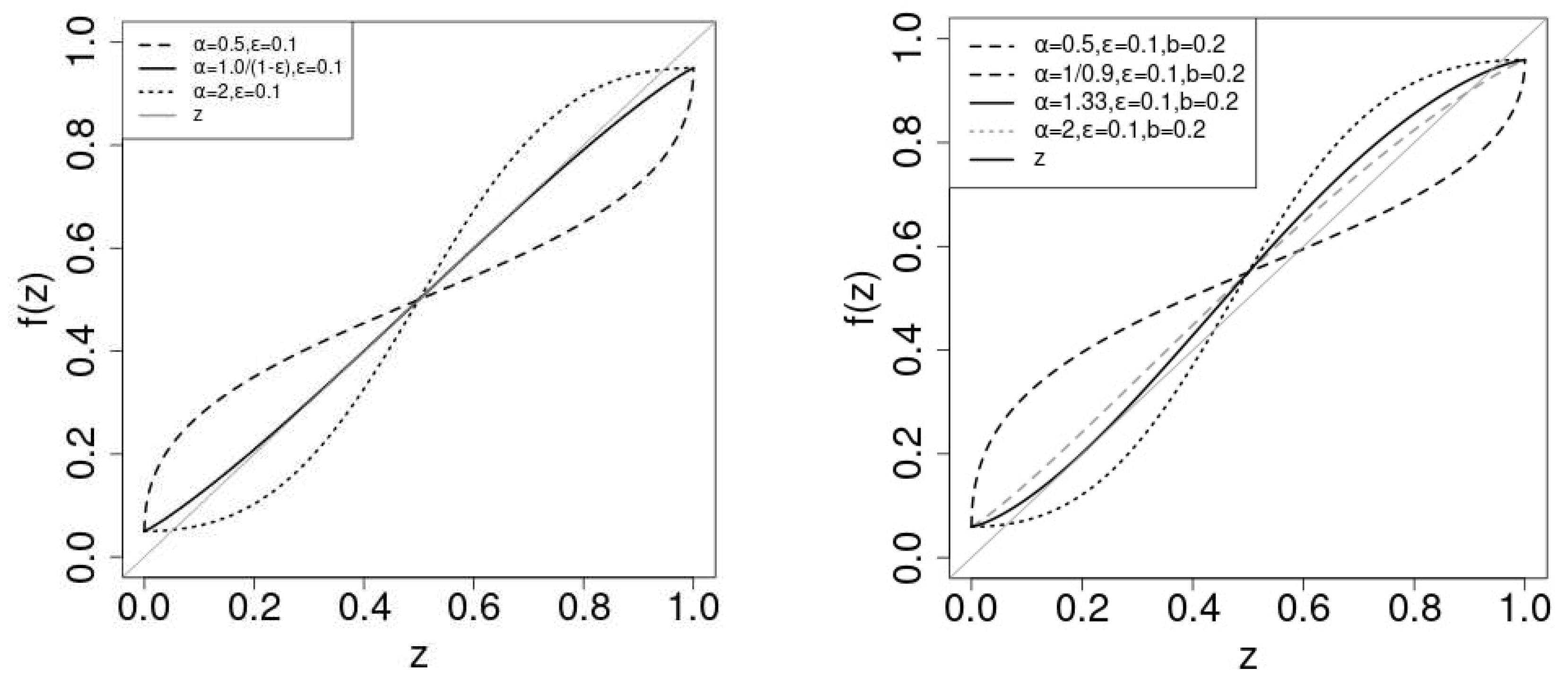
In the limit

N \to \infty

, the positive driving force

\frac{(1 - f (z))}{N \bar{f (Z (i, t))}}

in eq.(9) disappears. The system becomes

Z_{2}

symmetric and

z = 1 / 2

is a the solution as

f (1 / 2) = 1 / 2

. If N is finite, the positive driving force breaks the

Z_{2}

symmetry. We plot

(1 + b (1 - f (z)) f (z)

in Figure 1.

b > 0

corresponds with

1 / N \bar{f (Z (i, t))}

and

b ≃ 0.01 \sim 0.02

for

N = 100

and

\bar{f (Z (i, t)} = 1 / 2 \sim 1

. In the left and the right figure, we adopt

b = 0, ϵ = 0.1

and

b = 0.2, ϵ = 0.1

, respectively.

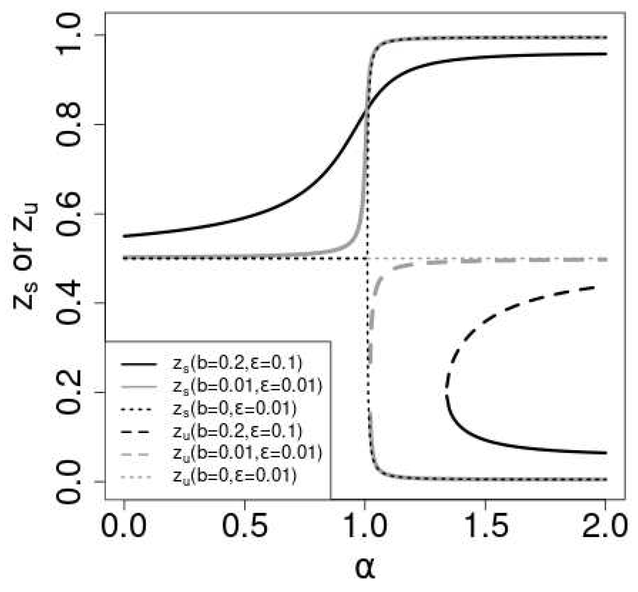
In the

Z_{2}

symmetric case (

b = 0

), the stability of the solution

z = 1 / 2

depends on the slope of

f (z)

z = 1 / 2

. As

f^{'} (1 / 2) = (1 - ϵ) α

, the critical value of

α

α_{c} = 1 / (1 - ϵ)

. If

α < (>) α_{c}

z = 1 / 2

is (un)stable. If

α = α_{c}

, the curve of

f (z)

is tangential to the diagonal.

Z (m, t)

converges to

1 / 2

for

α \leq α_{c}

, as

z = 1 / 2

is the unique stable solution

z_{s}

. For

α > α_{c}

, there appears two stable solutions

z_{s}, z_{s}^{'}

, one(

z_{s}^{'}

) is in

(0, 0.5)

and the other(

z_{s}

) is in

(0.5, 1.0)

z = 0.5

becomes the unstale solution

z_{u}

The dotted lines Figure 2 shows the solutions vs.

α

for the

Z_{2}

symmetric case. For

α < α_{c}

z = 1 / 2

(black dotted line) is the stable solution. For

α > α > c

z = 1 / 2

(gray dotted line) becomes unstable (

z_{u} = 1 / 2

) and two stable solution

z_{s}, z_{s}^{'}

departs from

z = 1 / 2

continuously with

α > α_{c}

. Which stable solution does

Z (m, t)

converge depends on the initial value of

Z (m, t_{0})

. In general, if

Z (m, t_{0})

is greater (smaller) than

1 / 2

, the probability of the convergence to 1 is greater (smaller) than

1 / 2

z_{u}

determines the "attractive domains" for the stable solutions

z_{s}, z_{s}^{'}

. The susceptibility of the expected value of

Z (m, t)

to the initial value

Z (m, t_{0})

is the order parameter of the non-linear Pólya urn[22,23]. As the order parameter is proportional to the difference of the two stable states, the order parameter is a continuous function of

α

and the phase transition is continuous.

In the

Z_{2}

asymmetric case (

b \neq 0

), for small values of

α

, there is a stable solution

z_{s}

in the range

(0.5, 1)

z_{s}

increase with

α

and at some critical value

α_{c}

α

, the curve

f (z) (1 + b (1 - f (z))

becomes tangential to the diagonal at

z = z_{t}

z_{t}

is known as touchpoint and to be stable[25]. As

α

continues to increase beyond

α_{c}

, two significant changes occur: a new stable solution

z_{s}^{'}

emerges from the touchpoint

z_{t}

, while an unstable solution

z_{u}

also becomes apparent.

When

α < α_{c}

, only one stable solution,

z_{s}

, exists within the range

1 / 2 < z_{s} < 1

. Conversely, for

α > α_{c}

, the specific stable solution to which

Z (m, t)

converges depends on the initial values of

Z (m, t_{0})

. At

α = α_{c}

, both the stable fixed point

z_{s}

and the touchpoint

z_{t}

remain stable. Which solution

Z (m, t)

converges to is determined by the initial values of

Z (m, t_{0})

in this case as well. For

α > α_{c}

, the situation mirrors that of

α = α_{c}

. Once

α \geq α_{c}

, the order parameter turns positive, and the phase transition becomes discontinuous.

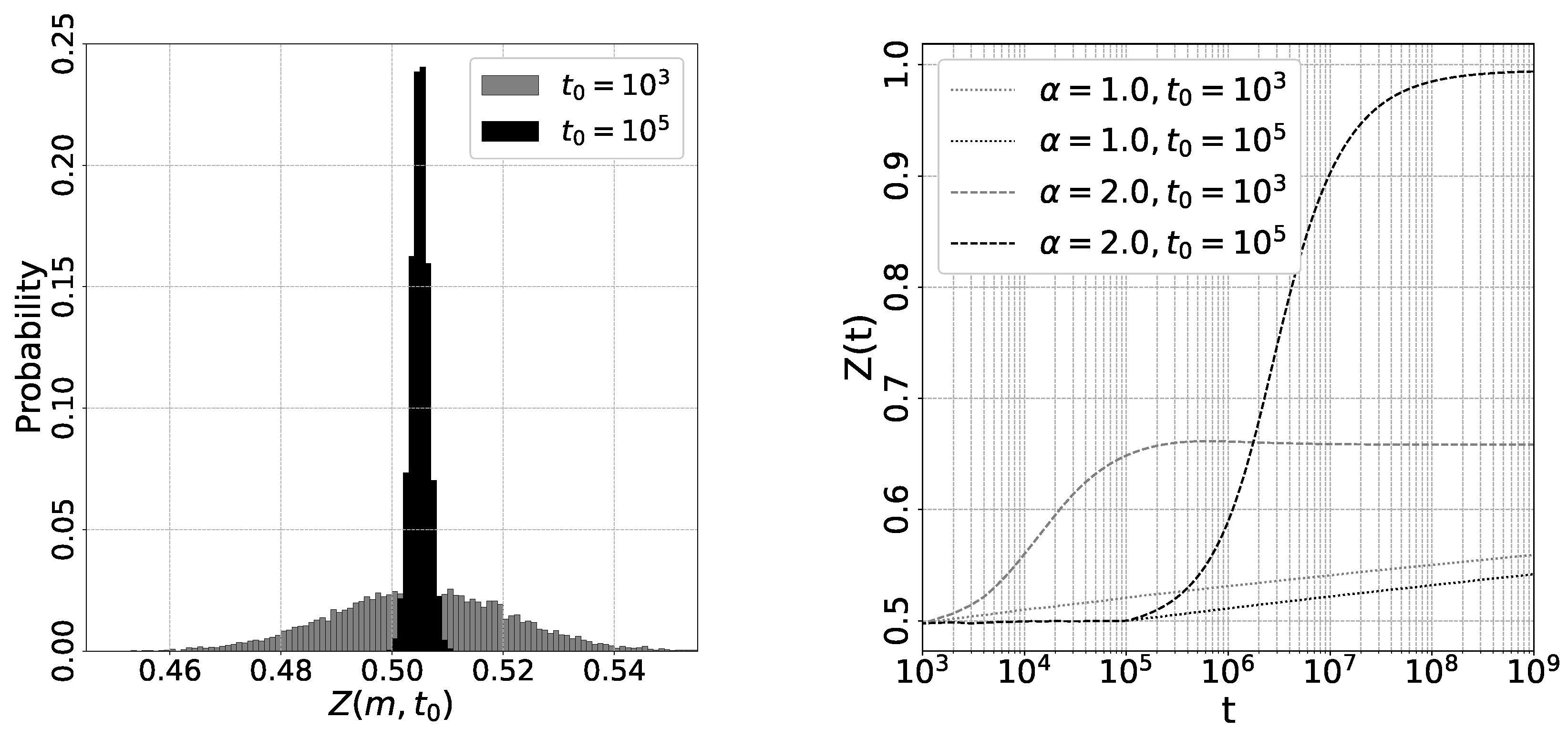
Figure 3 shows the results of the numerical studies in the limit

τ \to \infty

. We sampled a trajectory of

Z (m, t)

and

Z (t)

for

1 \leq t \leq 10^{9}

with

N = 10^{2}

and

ϵ = 0.01

. In the left figure, we present the distribution of

Z (m, t_{0})

for two different values of

t_{0}

, namely,

t_{0} \in 10^{3}, 10^{6}

. The mean value of

Z (m, t_{0})

is approximately

1 / 2 + 1 / 2 N

, which aligns with the theoretical predictions. The variance of

Z (m, t_{0})

is given by

1 / 4 t_{0}

, so the variance for

t_{0} = 10^{3}

is about

10^{3}

times larger than that for

t_{0} = 10^{6}

. Consequently, if we choose

t_{0} = 10^{3}

, a significant proportion of

m \in 1, \dots, N

will have

Z (m, t_{0}) < z_{u} ≃ 0.5

, resulting in a high probability that

Z (m, t)

converges to

z_{s}^{'} < 1 / 2

for

α = 2.0

. In such cases,

Z (t)

cannot reach 1 due to the convergence of

Z (m, t)

z_{s}^{'}

. On the other hand, if we set

t_{0} = 10^{5}

, the ratio of

m \in 1, \dots, N

with

Z (m, t_{0}) < z_{u} ≃ 0.5

is zero, ensuring that

Z (m, t)

always converges to

z_{s} > 1 / 2

. As a result,

Z (t)

monotonically increases towards 1 for

α = 2.0

. For

α = 1.0 < α_{c}

, where only one stable state

z_{s} ≃ 1

exists,

Z (m, t)

consistently converges to

z_{s}

. It’s evident that

Z (t)

monotonically approaches

z_{s}

with time for both

t_{0} = 10^{3}

and

t_{0} = 10^{5}

cases within the range

t \leq 10^{9}

. In the case of

α = 0.5

, where

z_{s} ≃ 0.5

Z (t)

experiences relatively little change

2.3. $τ < \infty$ case

In the case where

τ

is finite, we make the assumption that

t ≫ τ ≫ 1

and replace

D (t + 1)

with

N τ

in eq.(5) and eq.(7). This leads to the following equations:

\begin{matrix} d Z (m, t) & = & \frac{\bar{f (Z (i, t))}}{τ Z (t + 1)} ((1 + \frac{(1 - f (Z (m, t)))}{N \bar{f (Z (i, t))}}) f (Z (m, t)) - Z (m, t)) d t \\ + & (\frac{\bar{f (Z (i, t))}}{τ Z (t + 1)}) \sqrt{f (Z (m, t)) (1 - f (Z (m, t))} d W (t), m = 1, \dots, N \\ \frac{d}{d t} Z (t) & = & \frac{1}{τ} (\bar{f (Z (i, t))} - Z (t)) . \end{matrix}

(10)

The initial conditions for

Z (t)

and

Z (m, t)

t = t_{0} ≫ τ

are given as follows:

\begin{matrix} Z (t_{0}) & \sim & N (\frac{1}{2}, \frac{1}{8 N τ}), \\ Z (m, t_{0}) & \sim & N (\frac{1}{2} + \frac{1}{2 N}, \frac{1}{8 τ}) . \end{matrix}

(11)

The dynamics of

{Z (m, t)}_{m = 1, \dots, N}

are coupled through

Z (t)

and

\bar{f} (Z (i, t))

. To simplify and analyze this coupled system, we focus on the stationary state of

Z (m, t)

in the limit

t \to \infty

We anticipate that

Z (m, t) m = 1, \dots, N

will fluctuate around the stable fixed points of

f (z)

in the stationary state. As we observed earlier in the case of

τ \to \infty

, for

α < α_{c}

, there is only one stable fixed point, and for

α \geq α_{c}

, two stable fixed points exist, one of which is near 1. The stationary distribution is unimodal for

α < α_{c}

and bimodal for

α \geq α_{c}

. We denote the stationary distribution and the mean value of

Z (m, t)

P s t (z)

and

μ_{s t}

, respectively. As

f (Z (m, t))

is the probability for

X (m, t + 1) = 1

, we can assume

\bar{f (Z (i, t)} = Z (t) = μ_{s t}

in the stationary state. The SDEs in eq.(10) can be simplified as follows when replacing

\bar{f} (Z (i, t))

and

Z (t)

with

μ_{s t}

\begin{matrix} d Z (m, t) & = & \frac{1}{τ} ((1 + \frac{(1 - f (Z (m, t)))}{N μ_{s t}}) f (Z (m, 1)) - Z (m, t)) d t \\ + & \frac{1}{τ} \sqrt{f (Z (m, t)) (1 - f (Z (m, t))} d W (t) \\ = & A (Z (m, t)) d t + B (Z (m, t)) d W (t) \\ A (z) & = & \frac{1}{τ} ((1 + \frac{(1 - f (z))}{N μ_{s t}}) f (z) - z) \\ B (z) & = & \frac{1}{τ} \sqrt{f (z) (1 - f (z)} \end{matrix}

(12)

The stationary state with reflecting boundary conditions is determined by a potential solution[26], which can be expressed as:

\begin{matrix} P_{s t} (z) & \propto & \frac{1}{B {(z)}^{2}} exp (\int_{1 / 2}^{z} \frac{2 A (y)}{B {(y)}^{2}} d y) . \\ \frac{2 A (y)}{B {(y)}^{2}} & = & 2 τ \frac{f (y) - y}{f (y) (1 - f (y))} + \frac{2 τ}{N μ_{s t}} . \end{matrix}

(13)

The second term,

\frac{2 τ}{N μ_{s t}}

, arises from the

Z_{2}

symmetry-breaking field and causes a shift in the stationary distribution in the positive direction.

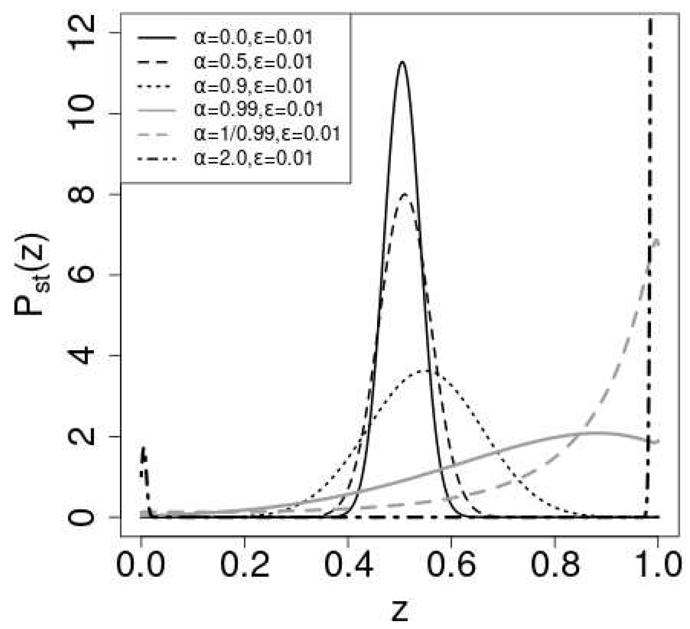
Figure 4 shows

P_{s t} (z)

in eq.(13) for

ϵ = 0.01, N = 10^{2}

μ_{s t}

is chosen so that the mean value of

P_{s t} (z)

coincides with

μ_{s t}

μ_{s t} = \int_{0}^{1} P_{s t} (z) z d z .

The parameters

(α, μ_{s t})

are

(0.0, 0.50)

(0.5, 0.51)

(0.9, 0.54)

(0.99, 0.67)

(1 / 0.99, 0.74)

and

(2.0, 0.54)

. As

α

increases, the peak position shifts in the positive direction, which can be expected by the dependence of the stable solution

z_{s}

α

in Figure 2. If

α = 1 / (1 - ϵ)

, the peak appears at

z = 1

, since there is only one stable fixed point near 1 in Figure 1. When

α = 2

, there are two stable fixed point and the stationary distribution is bimodal.

In order to derive the dependence of

μ_{s t}

and the variance of

P_{s t} (z)

α

, we assume that

Z (m, t)

fluctuates around

μ_{s t} ≃ \frac{1}{2}

for

α < α_{c}

. We linearrize

f (z)

in the vicinity of

z = 1 / 2

as,

f (z) = \frac{1}{2} + (1 - ϵ) α (z - \frac{1}{2}) .

We also approximate

B {(z)}^{2}

μ_{s t} (1 - μ_{s t}) = 1 / 4

P_{s t} (z)

becomes

P_{s t} (z) \propto exp (- \frac{{(z - (\frac{1}{2} + \frac{1}{2 N (1 - (1 - ϵ) α)}))}^{2}}{(\frac{2}{8 τ (1 - (1 - ϵ) α)})})

In the case

α = 0

, the ants does not observe the information of the pheromones and decide by themselves. The expected value and the variance are consistent with the results for the initial state in eq.(11). The expected value and the variance increase with

α

for

0 \leq α < 1 / (1 - ϵ)

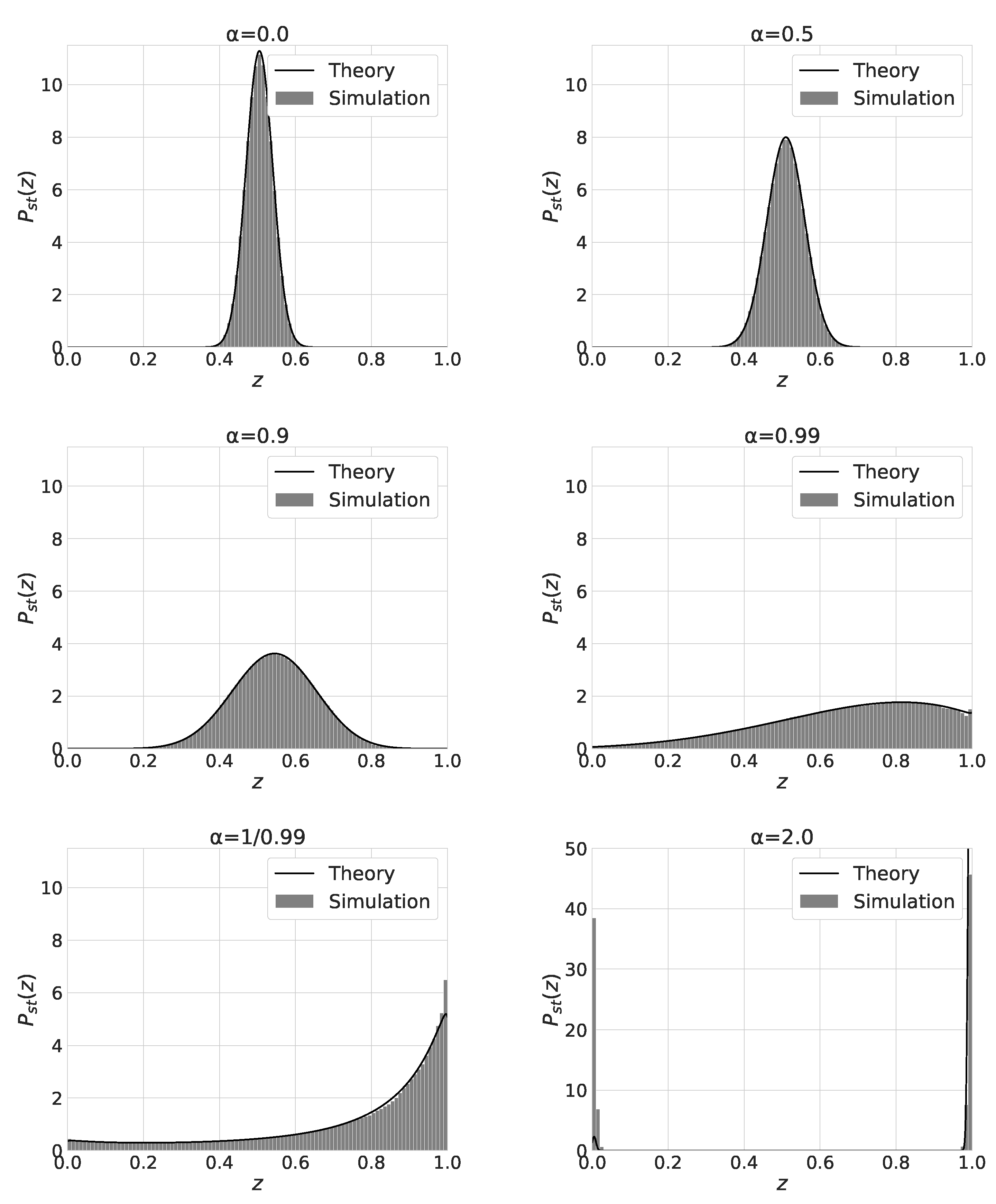
The shape of the stationary distribution changes from the monomodal shape for

α < α_{c}

to the bimodal shape for

α \geq α_{c}

. Figure 5 shows the stationary distribution of

Z (m, t)

for

α \in {0.0, 0.5, 0.9, 0.99, 1 / 0.99, 2.0}, ϵ = 0.01, τ = 100

and

N = 10^{2}

. We also plot

P_{s t} (z)

in eq.(13) with solid line curves. Except for the

α = 2.0

case, the numerical results agree with the theoretical ones. As

α

increases from 0 to

1 / 0.99

, the mean value and the variance of

Z (m, t)

increases. For

α = 1 / 0.99

, the distribution of

Z (m, t)

has a peak at

z = 1

. The distribution becomes bimodal and has two peaks near

z = 0

and

z = 1

for

α = 2

. For

α = 2.0

P_{s t} (z)

becomes bimodal and the equilibriation time to reach the stationary state becomes extremely long. We think this is the reason for the discrepancy between the numerical and theoretical results.

3. Discussion

We have studied a simple model for ACO and the convergence properties of the solutions. Ants answer many two-choice quizzes in sequence and deposit pheromone as they choose. As the amount of the pheromones is the number of correct answers, the following ants can receive information or hints about the correct choices. We have shown that the model reduces to a multi-variate non-linear Pólya urn process and the pheromones break the

Z_{2}

symmetry of the process. By varying the exponent

α

of the decision function of the ants, there occurs a phase transition about the convergence of the probability of choosing the correct answer for each question in the limit

τ \to \infty

. For

τ < \infty

, the change of the stationary distribution between the monomodal and the bimodal shape occurs as we vary

α

previous studies have adopted values of

α = 1

or smaller in solving real problems, like TSP. In

α

-annealing,

α

increases gradually, as shown in previous research[17]. In our study, we have shown that the duration of the period

α = 0

should be long enough to ensure that the initial value of

Z (m, t)

is in the attractive domain of the good stable state (

Z (m, t) > z_{u}

) in the case

τ = \infty

. Subsequently, with

α \geq 1

in effect,

Z (t)

converges to a value close to 1. In the case of

τ < \infty

, the timescale for pheromone evaporation, represented by

τ

, should be sufficiently long to maintain the same initial conditions. However,

Z (m, t)

does not converge to a specific value; instead, it follows a stationary distribution that exhibits both bimodal and monomodal shapes depending on the value of

α

. To achieve a distribution of

Z (t)

with a prominent peak near

z = 1

, the

α

-annealing process is an effective strategy. Both the stable solution

z_{s}

and the distribution of

Z (m, t)

suggest that, after a lengthy period with

α = 0

, it is advantageous to gradually increase

α

from 1. However, the efficiency of the annealing process depends on the specific problem being addressed. Future study should clarify the efficient

α

-annealing schedule.

Author Contributions

Conceptualization, S.M. and M.H.; methodology, S.M.; software, S.N.; validation, S.M. and S.N.; formal analysis, S.M. and K.N.; investigation, S.N.; resources, S.M.; data curation, S.N.; writing—original draft preparation, S.M.; writing—review and editing, S.M., S.N. K.N. and M.H.; visualization, S.M.; supervision, S.M.; project administration, S.M.; funding acquisition, S.M. All authors have read and agreed to the published version of the manuscript.

Funding

This research was funded by JPSJ KAKENHI [Grant No. 22K03445].

Data Availability Statement

We performed numerical simulations using Julia 1.7.3. The code is available on github[27].

Acknowledgments

This work was supported by JPSJ KAKENHI [Grant No. 22K03445].

Conflicts of Interest

The authors declare no conflict of interest.

Abbreviations

The following abbreviations are used in this manuscript:

SDE	stochastic differential equation
ACO	anto colony optimization
iid	independent and identically distributed

Appendix A

We assume

X (i, s)

are iid Bernoulli random variable with

P (X (i, s) = 1) = 1 / 2

for

i = 1, \dots, N

and

s \leq t_{0}

. As

E (X (i, s)) = 1 / 2

and

V (X (i, s)) = 1 / 4

, we have

\begin{matrix} E [S (t)] & = & \sum_{i = 1}^{N} \sum_{s = 1}^{t} E [X (i, s)] e^{- (t - s) τ} = \frac{1}{2} D (t) \\ V (S (t)) & = & \sum_{i = 1}^{N} \sum_{s = 1}^{t} V (X (i, s) e^{- (t - s) / τ}) = \frac{1}{4} N \sum_{s = 1}^{t} e^{- 2 (t - s) / τ} = \frac{1}{4} D_{h} (t) . \end{matrix}

Here, we define

D_{h} (t)

as,

D_{h} (t) = N \sum_{s = 1}^{t} e^{- 2 (t - s) / τ} .

Applying the central limit theorem, we can conclude that

Z (t) = S (t) / D (t)

behaves like a normal distribution, with its probability density function given by,

Z (t) \sim N (\frac{1}{2}, \frac{D_{h} (t)}{4 D {(t)}^{2}}) .

(A1)

S (m, t)

in eq.(2) is rewritten as

S (m, t) = \sum_{s = 1}^{t} X (m, s) (1 + \sum_{i \neq m} X (i, s)) e^{- (t - s) / τ} .

Conditional and unconditional expected values of

S (m, t)

are,

\begin{matrix} E [S (m, t) | {X (m, s)}_{s = 1, \dots, t}] & = & \sum_{s = 1}^{t} X (m, s) (\frac{1}{2} (N + 1)) e^{- (t - s) / τ} \\ E [S (m, t)] & = & E [E [S (m, t) | {X (m, s)}_{s = 1, \dots, t}]] = (\frac{1}{4} + \frac{1}{4 N}) D (t) . \end{matrix}

Conditional variance of

S (m, t)

V (S (m, t) | {X (m, s)}_{s = 1, \dots, t}) = \sum_{s = 1}^{t} X (m, s) \frac{1}{4} (N - 1) e^{- 2 (t - s) / τ}

Unconditional variance is

\begin{matrix} V (S (m, t)) & = & E [V (S (m, t) | {X (m, s)}_{s = 1, \dots, t})] + V (E [S (m, t) | {X (m, s)}_{s = 1, \dots, t}]) \\ = & (\frac{1}{16} N + \frac{1}{4} - \frac{1}{16 N}) D_{h} (t) ≃ \frac{1}{16} N \cdot D_{h} (t) . \end{matrix}

We estimate the variance of

Z (m, t) = S (m, t) / S (t)

by neglecting the fluctuation of

S (t)

as,

V (Z (m, t)) ≃ \frac{V (S (m, t))}{E {[S (t)]}^{2}} = \frac{N D_{h} (t)}{4 D {(t)}^{2}} .

By the central limit theorem,

Z (m, t) = S (m, t) / S (t)

behaves as

Z (m, t) \sim N (\frac{1}{2} + \frac{1}{2 N}, \frac{N D_{h} (t)}{4 D {(t)}^{2}}) .

(A2)

References

Galam, S. Sociophysics: A review of Galam models. Int. J. Mod. Phys. C 2008, 19, 409–440. [Google Scholar] [CrossRef]
Galam, S. A physicist’s modeling of psycho-political phenomena; Springer: New York, 2012. [Google Scholar]
Galam, S. Majority rule, hierarchical structures and democratic totalitarism: a statistical approach. J. of Math. Psychology 1986, 30, 426–434. [Google Scholar] [CrossRef]
Arthur, W.B. Competing Technologies, Increasing Returns, and Lock-In by Histrical Events. Econ. Jour. 1989, 99, 116–131. [Google Scholar] [CrossRef]
Bikhchandani, S.; Hirshleifer, D.; Welch, I. A Theory of Fads, Fashion, Custom, and Cultural Changes as Informational Cascades. J. Polit. Econ. 1992, 100, 992–1026. [Google Scholar] [CrossRef]
Mori, S.; Hisakado, M.; Takahashi, T. Phase transition to two-peaks phase in an information cascade voting experiment. Phys. Rev. E 2012, 86, 026109–026118. [Google Scholar] [CrossRef] [PubMed]
Nakayama, K.; Hisakado, M.; Mori, S. Nash Equilibrium of Social-Learning Agents in a Restless Multiarmed Bandit Game. Sci.Rep. 2017, 7, 1937. [Google Scholar] [CrossRef] [PubMed]
Galam, S.; Cheon, T. Asymmetric contrarians in opinion dynamics. Entropy 2020, 22(1), 25. [Google Scholar] [CrossRef] [PubMed]
Kirman, A. Ants, rationality and recruitment. Q. J. Econ. 1993, 108, 137–156. [Google Scholar] [CrossRef]
Hisakado, M.; Mori, S. Information cascade, Kirman’s ant colony model, and kinetic Ising model. Physica A 2015, 417, 63–75. [Google Scholar] [CrossRef]
Pasteels, J.; Deneubourg, J.; Detrain, C. Information processing in social insects; Birkhauser Verlag: Basel, 2007. [Google Scholar]
Camazine, S.; Deneubourg, J. Self-organization in biological systems; Princeton University Press: NJ, 2001. [Google Scholar]
Dorgio, M. Optimization, learning and Natural algorithms. PhD thesis, Poltecnico di Milan, 1992. [Google Scholar]
Dorgio, M.; Caro, G.D. The ant colony meta-heuristic. In Proceedings of the New Ideas in Optimization; Corne, D., Dorgio, M.M., Glover, F., Eds.; McGraw Hill: London, 1999; pp. 11–32. [Google Scholar]
Cordon, O.; Herrera, F.; Stutzle, T. A review on the ant colony optimization metaheuristic. Mathware and Soft Computing 2002, 9, 141–175. [Google Scholar]
Dorgio, M.; Gambardella, L. Ant Colonies for the Travelling Salesman Problem. Biosystem 1997, 43, 73–81. [Google Scholar] [CrossRef] [PubMed]
Mayer, B. On the convergence behaviour of ant colony search. Complexity 2005, 12, 73–81. [Google Scholar]
Gutjahr, W. ACO algorithms with guaranteed convergence to the optimal solution. Information Processing Letters 2002, 82, 145–153. [Google Scholar] [CrossRef]
Nakamichi, Y.; Arita, T. Diversity control in ant colony optimization. Artificail Life and Robotics 2001, 7, 198–204. [Google Scholar] [CrossRef]
Randall, M.; Tonkes, E. Intensification and diversification strategies in ant colony system. Complexity International 2002, 9, 1–7. [Google Scholar]
Hisakado, M.; Hino, M. Between Ant Colony Optimization and Genetic Algorithm. IPSJ TOM 2016, 9(3), 8–14. [Google Scholar]
Mori, S.; Hisakado, M. Correlation function for generalized Pólya urns: Finite-size scaling analysis. Phys.Rev. E 2015, 92, 052112–052121. [Google Scholar] [CrossRef] [PubMed]
Nakayama, K.; Mori, S. Universal function of the non-equilibrium phase transition of nonlinear Pólya urn. Phys. Rev.E 2021, 104, 014109–014118. [Google Scholar] [CrossRef] [PubMed]
Hill, B.; Lane, D.; Sudderth, W. A strong law for some generalized urn processes. Ann. Probab. 1980, 8, 214–226. [Google Scholar] [CrossRef]
Pemantle, R. When are touchpoints limits for generalized Pólya urns? Proc. Amer. Math. Soc. 1991, 113, 235–243. [Google Scholar]
Gardiner, C. Stochastic Methods: A handbook for the Natural and Social Science, 4th ed.; Springer: Berlin, 2009. [Google Scholar]
Sampling programs for Phase transition in ACO. Available online: https://github.com/LABO-M/ACO.

Figure 1. Left: Plot of

f (z)

in eq.(4) vs. z with

ϵ = 0.1

. Right: Plot of

(1 + b (1 - f (z)) f (z)

vs. z with

ϵ = 0.1, b = 0.2

. In both figures, we use

α = 0.5

(black dashed line),

1.0

(black solid line) and

2.0

(black dotted line). In the right figure, we also plot

(1 + b (1 - f (z)) f (z)

for

α = 1 / (1 - ϵ)

(gray dashed line) We also plot z (gray solid line) to see the fixed point of

f (z)

Figure 1. Left: Plot of

f (z)

in eq.(4) vs. z with

ϵ = 0.1

. Right: Plot of

(1 + b (1 - f (z)) f (z)

vs. z with

ϵ = 0.1, b = 0.2

. In both figures, we use

α = 0.5

(black dashed line),

1.0

(black solid line) and

2.0

(black dotted line). In the right figure, we also plot

(1 + b (1 - f (z)) f (z)

for

α = 1 / (1 - ϵ)

(gray dashed line) We also plot z (gray solid line) to see the fixed point of

f (z)

Figure 2. Plot of the stale solutions

z_{s}

for

b = 0.2, ϵ = 0.1

(black solid line),

b = 0.01, ϵ = 0.01

(gray solid line) and

b = 0, ϵ = 0.01

(black dotted line). Plot of the unstable solutions

z_{u}

for

b = 0.2, ϵ = 0.1

(black broken line),

b = 0.01, ϵ = 0.01

(gray broken line) and

b = 0, ϵ = 0.01

(gray dotted line).

Figure 2. Plot of the stale solutions

z_{s}

for

b = 0.2, ϵ = 0.1

(black solid line),

b = 0.01, ϵ = 0.01

(gray solid line) and

b = 0, ϵ = 0.01

(black dotted line). Plot of the unstable solutions

z_{u}

for

b = 0.2, ϵ = 0.1

(black broken line),

b = 0.01, ϵ = 0.01

(gray broken line) and

b = 0, ϵ = 0.01

(gray dotted line).

Figure 3. Left. Plot of the initial distribution of

Z (m, t_{0})

for the limit

τ \to \infty

. We set

α = 0, ϵ = 0.01

and

N = 10^{2}

t_{0} = 10^{3}

and

t_{0} = 10^{5}

. Right. Plot of

Z (t)

vs. t for

α = 0.5

(solid line),

1.0

(dotted line) and

2.0

(dashed line).

t_{0} = 10^{3}

(gray) and

10^{5}

(black).

Figure 3. Left. Plot of the initial distribution of

Z (m, t_{0})

for the limit

τ \to \infty

. We set

α = 0, ϵ = 0.01

and

N = 10^{2}

t_{0} = 10^{3}

and

t_{0} = 10^{5}

. Right. Plot of

Z (t)

vs. t for

α = 0.5

(solid line),

1.0

(dotted line) and

2.0

(dashed line).

t_{0} = 10^{3}

(gray) and

10^{5}

(black).

Figure 4. Plot of the stationary state of eq.(13). We adopt

N = 10^{2}

and

ϵ = 0.01

. The parameters

(α, μ_{s t})

are

(0.0, 0.50)

(black solid line),

(0.5, 0.51)

(black dashed line),

(0.9, 0.54)

(black dotted line),

(0.99, 0.67)

(gray solid line),

(1 / 0.99, 0.74)

(gray dashed line) and

(2.0, 0.54)

(gray chain line).

Figure 4. Plot of the stationary state of eq.(13). We adopt

N = 10^{2}

and

ϵ = 0.01

. The parameters

(α, μ_{s t})

are

(0.0, 0.50)

(black solid line),

(0.5, 0.51)

(black dashed line),

(0.9, 0.54)

(black dotted line),

(0.99, 0.67)

(gray solid line),

(1 / 0.99, 0.74)

(gray dashed line) and

(2.0, 0.54)

(gray chain line).

Figure 5. Plots of the distribution of

Z (m, t = 10^{5})

. We set

τ = 10^{2}

t_{0} = 10^{5}

and

ϵ = 0.01

. Initial state

α = 0

(Upper left),

α = 0.5

(Upper Right) and

α = 0.9

(Middle left),

α = 0.95

(Middle right),

α = 1.0

(Lower left) and

α = 2.0

(Lower Right).

Figure 5. Plots of the distribution of

Z (m, t = 10^{5})

. We set

τ = 10^{2}

t_{0} = 10^{5}

and

ϵ = 0.01

. Initial state

α = 0

(Upper left),

α = 0.5

(Upper Right) and

α = 0.9

(Middle left),

α = 0.95

(Middle right),

α = 1.0

(Lower left) and

α = 2.0

(Lower Right).

Disclaimer/Publisher’s Note: The statements, opinions and data contained in all publications are solely those of the individual author(s) and contributor(s) and not of MDPI and/or the editor(s). MDPI and/or the editor(s) disclaim responsibility for any injury to people or property resulting from any ideas, methods, instructions or products referred to in the content.

© 2023 by the authors. Licensee MDPI, Basel, Switzerland. This article is an open access article distributed under the terms and conditions of the Creative Commons Attribution (CC BY) license (http://creativecommons.org/licenses/by/4.0/).

Copyright: This open access article is published under a Creative Commons CC BY 4.0 license, which permit the free download, distribution, and reuse, provided that the author and preprint are cited in any reuse.

MDPI Initiatives

Important Links

Choose an area of interest and we will send you notifications of new preprints at your preferred frequency.

Disclaimer

Phase Transition in Ant Colony Optimization

Abstract

0. Introduction

1. Materials and Methods

1.1. Stochastic Differential equation

2. Results

2.1. Initial distribution of { Z ( m , t ) }

2.2. τ → ∞ case

2.3. τ < ∞ case

3. Discussion

Author Contributions

Funding

Data Availability Statement

Acknowledgments

Conflicts of Interest

Abbreviations

Appendix A

References

MDPI Initiatives

Important Links

Subscribe

2.1. Initial distribution of ${Z (m, t)}$

2.2. $τ \to \infty$ case

2.3. $τ < \infty$ case