Autonomous Optimal Absolute Orbit Keeping Through Formation-Flying Techniques

Preprint

Article

Autonomous Optimal Absolute Orbit Keeping Through Formation-Flying Techniques

Altmetrics

Downloads

Views

Comments

A peer-reviewed article of this preprint also exists.

Ahmed Mahfouz^*,

Gabriella Gaias,

D. M. K. K. Venkateswara,

Holger Voos

Ahmed Mahfouz^*,

Gabriella Gaias,

D. M. K. K. Venkateswara,

Holger Voos

This version is not peer-reviewed

Submitted:

17 October 2023

Posted:

19 October 2023

You are already at the latest version

Alerts

Abstract

In this paper, the problem of autonomous optimal absolute orbit keeping for a satellite mission in Low Earth Orbit using electric propulsion is considered. The main peculiarity of the approach is to support small satellite missions in which the platform is equipped with a single thruster nozzle which provides acceleration on a single direction at a time. This constraint implies that an attitude maneuver is necessary before or during each thrusting arc to direct the nozzle into the desired direction. In this context, an attitude guidance algorithm specific for the orbit maneuver has been developed. A Model Predictive Control scheme is proposed, where the attitude kinematics are coupled with the orbital dynamics in order to obtain the optimal guidance profiles in terms of satellite state, reference attitude, and thrust magnitude. The proposed control scheme is developed exploiting Formation Flying techniques where the reference orbit is that of a virtual spacecraft that the main satellite is required to rendezvous with. In addition to the controller design, the closed loop configuration is presented supported by numerical simulations. The efficacy of the proposed autonomous orbit keeping approach is shown in several application scenarios.

Keywords:

Subject: Engineering - Aerospace Engineering

1. Introduction

In recent years, the adoption of electric propulsion is becoming more popular among small satellite designers [1]. This trend is driven by the fact that electric propulsion systems are generally more sustainable and more efficient in terms of propellant usage in comparison to chemical propulsion ones. Moreover, electric thrusters could support large maneuvers while being smaller in size and lighter in weight than its chemical counterparts. This, in-turn, can allow the allocation of more space/weight for the payload, and in many cases permits successful integration within some launchers that would be infeasible for the satellite if it were equipped with chemical thrusters.

To further reduce the mass, size, and power requirements of the orbital control system, many design teams choose to equip their spacecraft with a single electric thruster. Examples of such satellites include Triton-X Medium and Heavy [2], and the Gravity Field and Steady-State Ocean Circulation Explorer (GOCE) satellite [3]. Thanks to the simple design of such propulsion system, the satellite could be designed with a high level of flexibility which permits the accommodation of larger payloads. However, having only one thruster onboard comes with its own challenges. For instance, the guidance and control schemes have to be optimized for the unidirectional thrust system, in the sense that attitude and orbit control systems have to be coupled to ensure that the thruster is always aligned with the desired firing direction. Moreover, this need becomes more relevant for orbit corrections that have to be performed on a limited time frame and/or when a very low thrust level is available.

This paper is focusing on optimal absolute orbit keeping for LEO satellites equipped with a single electric thruster. The problem is approached using formation flying techniques, meaning that the adopted satellite is assumed to be flying in a formation with a virtual chief. Namely, when an orbit transfer maneuver is defined, the chief’s orbit is set as the target one, and the satellite is ultimately required to rendezvous with the virtual chief. On the one hand, opting for the exploitation of FF techniques enables the developed guidance and control schemes to be directly used in multi-satellite scenarios. On the other hand, the absolute orbit control problem can be efficiently tackled by linearizing the orbital dynamics around the reference desired trajectory. In this context, the relative orbit between the satellite and the virtual target can be formulated using the Relative Orbital Elements (ROE), which render the linearized relative orbital dynamics with high levels of accuracy for neighbouring orbits.

Many contributions into autonomous absolute orbit keeping for LEO satellites have been introduced over the last few decades [4,5,6,7]. Among the many, formation flying techniques were used for absolute orbit control in [8] , where the spacecraft had to maintain its ground track close to a reference trajectory computed as the orbit of a virtual chief satellite. A specific set of variables is used to parameterize the relative motion and linear and quadratic optimal regulators are employed. In [9,10] formation reconfiguration with realistic mission constraints is considered. The proposed control schemes on these two articles relied on candidate Lyaponuv functions that comprised artificial potential around the prohibited areas (in the decision variables’ space), which guided the main satellite to follow feasible trajectories without having to solve an optimization problem. The main drawback of this approach is that the trajectories followed by the spacecraft are neither fuel- nor time-optimal. All the aforementioned contributions considered only satellites with 3D thrusting capabilities, and most of them adopted impulsive thrust. One mission which adopted a single impulsive thruster is the Autonomous Vision Approach Navigation and Target Identification (AVANTI) experiment [11] where a specific guidance scheme had been adopted to include no-control windows that allowed the re-orientation of the available nozzle [12,13]. The only research, up to the authors’ knowledge, that addresses the problem of absolute orbit control for unidirectional-low-thrust satellites is [14], nonetheless it does not consider the coupled attitude evolution, making such approach not suitable for prompt orbit corrections. Moreover, in [14] both the navigation and the actuator errors are also not considered.

In this paper, a Model Predictive Control (MPC) scheme is proposed which couples the attitude and the relative translational equations, where the relative dynamics are formulated in the ROE space. In this setting, the MPC uses an attitude control surrogate model to emulate the functioning of the satellite’s attitude control system as well as the ROE-based linearized relative dynamical model to predict the satellite’s future roto-translational state. The output of the MPC is a tuple which contains the optimal acceleration that should be provided by the thruster as well as the optimal desired attitude which the attitude control system needs to steer the satellite to. The overall cost function of the MPC at each receding horizon is a trade-off between delta-V optimality, time optimality, and attitude effort optimality, and is specifically designed for the purpose of small orbit changes (less than 1 km) as typically encountered in absolute orbit control problems around a reference orbit. The original contributions of the proposed approach are,

considering the coupled attitude/relative orbit problem in the control loop;
proposing a MPC scheme for a satellite with a unidirectional propulsion system where the thrust can be provided also during the slew maneuvers.

Thanks to the publicly available detailed specifications of Triton-X Heavy (referred to as Triton-X in the sequel), it is assumed to be the employed satellite for most of the numerical simulations in this work. Indeed, the proposed control algorithm in this paper is not limited to Triton-X. It was used as an example to showcase that the MPC scheme can be applied to a satellite with realistic specifications.

The following section of this paper introduces the formulation of the relative orbital dynamics in the ROE space as well as the adopted surrogate model for the attitude control system. In Section 3, the MPC problem is formally established in the sense that the employed cost function is introduced and the inherent constraints of the problem in hand are presented. The problem of MPC parameters tuning as well as the module execution logic of the closed control loop are discussed in the same section. The stability of the proposed MPC scheme is then tested by means of Monte-Carlo simulation in Section 4, and the proposed MPC is benchmarked against that which is introduced in [14].

2. Mathematical models

In this section, the dynamical models used in developing the control schemes are presented. At first, the reference frames used in the research are identified, then the relative orbital dynamics of the deputy spacecraft with respect to the chief (virtual) satellite are shown, and finally the attitude kinematics are introduced.

The following reference frames are used in developing the dynamic models as well as the control scheme.

Earth-Centered-Inertial frame

The employed Earth-Centered-Inertial (ECI) reference frame, $F^{i}$ , is defined by True-of-Date coordinate system with its origin at the center of the Earth, its x-axis along the true vernal equinox at the current epoch, its z-axis is aligned with the true rotation axis at the current epoch, while its y-axis completes the right-handed triad. A vector expressed in the ECI frame is signified by the ${(\cdot)}^{i}$ superscript.
Satellite-body-fixed frame

The body-fixed reference frame, $F^{b}$ , is a reference frame attached to the spacecraft in question with the origin at the satellite’s center of mass. One common choice of the directions of the three axes is along the three principal axes of inertia of the satellite. A vector expressed in the body-fixed frame of the satellite will have the superscript ${(\cdot)}^{b}$ .
Radial-Transversal-Normal frame

The Radial-Transversal-Normal (RTN) frame, $F^{r}$ is centered on the center of mass of the chief satellite, where the x-axis of the RTN frame is defined to be along the position vector of the chief satellite, positive towards the Zenith direction, the z-axis is directed along the chief’s orbital angular momentum vector, and the y-axis completes the right-handed set. In the sequel, a vector expressed in the RTN frame is signified by the ${(\cdot)}^{r}$ superscript.

2.1. Relative orbital dynamics

The orbital motion of a satellite under the gravitational influence of a major body (e.g. the Earth) can be parameterized in a planet-centered inertial frame by the following set of orbital elements,

α : = [\begin{matrix} a \\ θ \\ e_{x} \\ e_{y} \\ i \\ Ω \end{matrix}],

(1)

where a is the semi-major axis,

θ = M + ω

, is the argument of latitude with M being the mean anomaly and

ω

being the argument of periapsis,

e : = {[\begin{matrix} e_{x} & e_{y} \end{matrix}]}^{⊺} = {[\begin{matrix} e cos ω & e sin ω \end{matrix}]}^{⊺}

, is the eccentricity vector with e being the orbital eccentricity, i is the orbital inclination, and

Ω

is the Right Ascension of the Ascending Node (RAAN). If a Cartesian state vector is used, then the motion of the satellite in the planet-centered inertial frame is parameterized by,

x^{i} : = {[\begin{matrix} {r^{i}}^{⊺} & {v^{i}}^{⊺} \end{matrix}]}^{⊺}

, where

r^{i}

and

v^{i}

are the absolute position and velocity vectors. These latter are related to the orbital elements through a set of non-linear equations. Spacecraft position and velocity transform into osculating orbital elements, which in the remainder of this work will be denoted by

\tilde{α}

. Mean orbital elements, denoted by

α

, are to be intended as one-orbit averaged elements, where the short- and long-term oscillations generated by the

J_{2}

harmonic of the Earth gravitational potential are removed. Mean/osculating elements’ conversions are performed through the transformations developed in [15].

The relative motion between a deputy and a chief spacecraft can be described by the dimensionless quasi-nonsingular Relative Orbital Elements (ROE) vector which is a nonlinear transformation of the orbital elements vector introduced in (1),

δ α : = [\begin{matrix} δ a \\ δ λ \\ δ e_{x} \\ δ e_{y} \\ δ i_{x} \\ δ i_{y} \end{matrix}] = [\begin{matrix} Δ a / a_{c} \\ Δ θ + Δ Ω cos i_{c} \\ Δ e_{x} \\ Δ e_{y} \\ Δ i \\ Δ Ω sin i_{c} \end{matrix}],

(2)

where

δ a

is the relative semi-major axis,

δ λ

is the relative mean longitude,

δ e : = {[\begin{matrix} δ e_{x} & δ e_{y} \end{matrix}]}^{⊺}

is the relative eccentricity vector, and

δ i : = {[\begin{matrix} δ i_{x} & δ i_{y} \end{matrix}]}^{⊺}

is the relative inclination vector. It is important to note that here, and in the sequel, the subscript

{(\cdot)}_{d}

denotes a quantity related to the deputy satellite, while the subscript

{(\cdot)}_{c}

is used for chief-related quantities. Moreover,

δ (\cdot)

signifies a relative quantity between the deputy and the chief which is not necessarily the arithmetic difference between that of the deputy and that of the chief, while

Δ (\cdot)

signifies the arithmetic difference between

{(\cdot)}_{d}

and

{(\cdot)}_{c}

, i.e.

Δ (\cdot) : = {(\cdot)}_{d} - {(\cdot)}_{c}

. As for absolute elements, osculating ROE are denoted by

δ \tilde{α}

, whereas mean ROE are expressed as

δ α

. Both sets are computed from the corresponding osculating/mean orbital elements’ set by means of (2).

One of the advantages of the adopted ROE is that they provide a direct insight on the shape of the relative orbit, unlike the relative position and velocity vectors which need to be integrated over time in order to obtain a intuition of the relative orbit. Given the set of ROE in (2), the shape of the relative orbit can be constructed as an ellipse, in both, the Transversal-Radial and the Normal-Radial planes (see Figure 1).

In this work, the adopted relative dynamics are the same as in [16], where the dynamics of the ROE are linearized to the first order and the secular effect due to

J_{2}

zonal harmonic is included in the relative motion. The following assumptions apply:

Neighbouring orbits of the deputy and the chief,
Near circular chief’s orbit.

The solution to the linear system under the influence of a constant input acceleration is given in the following form,

δ α (t_{k + 1}) = Φ (t_{k}, t_{k + 1}) δ α (t_{k}) + Ψ (t_{k}, t_{k + 1}) u^{r} (t_{k}, t_{k + 1}),

(3)

where

Φ (t_{k}, t_{k + 1}) \in R^{6 \times 6}

is the State Transition Matrix (STM) between the two time instants,

t_{k}

and

t_{k + 1}

Ψ (t_{k}, t_{k + 1}) \in R^{6 \times 3}

is the convolution matrix between the same two time instants, and

u^{r} (t_{k}, t_{k + 1}) \in R^{3}

is the acceleration vector in

F^{r}

which is constant over the period

[t_{k}, t_{k + 1})

. The reader is referred to [16] for the detailed expressions of

Φ (t_{k}, t_{k + 1})

and

Ψ (t_{k}, t_{k + 1})

In the sequel, and in order to simplify the representation of equations, the following notations are used,

Φ_{k | k + 1} \equiv Φ (t_{k}, t_{k + 1})

Ψ_{k | k + 1} \equiv Ψ (t_{k}, t_{k + 1})

δ α_{k} \equiv δ α (t_{k})

, and

u_{k | k + 1}^{r} \equiv u^{r} (t_{k}, t_{k + 1})

2.2. Attitude kinematics

Given that the adopted satellite is equipped with only one thruster, continuous attitude maneuvers are necessary in order to direct the thruster to the desired direction during time-extended orbit maneuvers, which are likely to occur with the available low-thrust level. In this work, it is assumed that the attitude control system of the adopted satellite is capable to track a desired attitude profile. The specifications of the attitude control system are assumed to be the same as that of Triton-X which can be obtained from its publicly available brochure1. A surrogate model for the Attitude Determination and Control System (ADCS) is presented here, but first, the attitude kinematics are introduced.

Letting

q^{x y} \in Q

, with

Q : = {q \in R^{4} : ∥q∥ = 1}

be the unit quaternion that rotates any vector,

v \in R^{3}

, from one reference frame

F^{y}

to another frame

F^{x}

, through,

v^{x} = q^{x y} \circ v^{y} \circ {\tilde{q}}^{x y},

(4)

where ∘ is the quaternion multiplication operator, and

{\tilde{q}}^{x y}

is the quaternion conjugate of

q^{x y}

. Equivalently, the attitude rotation can be performed using the Direction Cosine Matrix (DCM),

A (q^{x y}) \in A

, with

A : = {A \in R^{3 \times 3} : A^{⊺} A = I}

, (see Appendix A in [17]), as follows,

v^{x} = A (q^{x y}) v^{y} .

(5)

The attitude kinematics of a rigid body can be described as follows [18]:

{\dot{q}}^{x y} = \frac{1}{2} q^{x y} \circ ω^{y},

(6)

where

ω^{y} \in R^{3}

is the angular velocity of frame

F^{y}

with respect to frame

F^{x}

, expressed in

F^{y}

Letting

q \equiv q (t) = q^{r b} (t)

ω \equiv ω (t) = ω^{b} (t)

, and letting

q_{r} \equiv q_{r} (t)

being the desired/reference quaternion at time t, (6) can be written as,

\dot{q} = \frac{1}{2} q \circ ω,

(7)

and the error quaternion signal,

q_{e}

is defined, in terms of the current attitude and the reference one, as,

q_{e} : = [\begin{matrix} q_{e, 0} \\ q_{e} \end{matrix}] : = {\tilde{q}}_{r} \circ q .

(8)

The ultimate behaviour of an ADCS would be to force the error quaternion to asymptotically approach either

{[\begin{matrix} 1 & 0 & 0 & 0 \end{matrix}]}^{⊺}

{[\begin{matrix} - 1 & 0 & 0 & 0 \end{matrix}]}^{⊺}

, which could be achieved through forcing the angular velocity,

ω

, profile to follow,

ω = - K q_{e, 0} q_{e},

(9)

where K is a positive control gain. The rationale behind why

ω

profile is plausible is given in Appendix A.

An additional operational constraint is imposed on the ADCS which dictates that the angular rate around any axis does not exceed the maximum allowable angular rate, i.e.

∥ω∥ \leq ω_{m a x}

. To be compliant with the attitude control specifications of Triton-X, the value of K is set to

0.2

, while the value of

ω_{m a x}

is set to 2 deg/sec. Indeed,

ω_{m a x}

could be found directly in the data-sheets. The numerical value of K, instead, has been assessed through numerical simulations in order to properly emulate the behavior of Triton-X ADCS, based on the time duration to perform a 60 degrees slew.

Substituting from (9) into (7), the adopted surrogate model for the ADCS is obtained,

\dot{q} = - \frac{1}{2} K q_{e, 0} q \circ q_{e} .

(10)

One thing that has to be acknowledged is that the attitude and angular velocity profiles of the actual satellite could differ slightly from the profiles generated by the surrogate model assumed here, depending on the exact quaternion feedback regulator used by the ADCS as well as the exact inertia tensor of the satellite. Nonetheless, changing the value of K could bring the attitude and angular velocity profiles of the surrogate model very close to that of the actual ADCS. This claim could be verified through benchmarking the surrogate model against a full attitude control system which uses one of the commonly used feedback regulator proposed in [19], and the results are depicted in Figure 2. It is to be noted that the initial and reference quaternions are randomly chosen for the simulation in Figure 2. Moreover, the subscript

{(\cdot)}_{full}

refers to a quantity relating to the full attitude control model, while the subscript

{(\cdot)}_{surr}

refers to surrogate model quantities.

3. Model-Predictive Control

3.1. MPC problem formulation

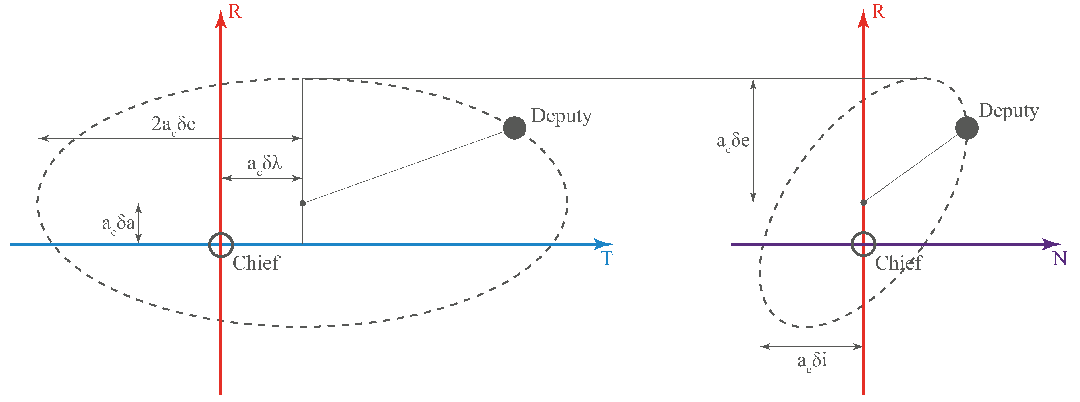
The Model Predictive Control problem is, in its essence, a recurring optimization problem that searches for the optimal control input over the receding control horizon, and in most cases, solves as well for the state variables over the prediction horizon. Only the first control input in the control horizon is realized by the actuators. In the context of our problem, attitude dynamics are coupled with the ROE-based relative translational motion, and the state vector is set to,

s = [\begin{matrix} δ α \\ q \end{matrix}],

(11)

where the dynamics of the state vector are described by (3) and (10). The control input, on the other hand, is set to

u = [\begin{matrix} u \\ q_{r} \end{matrix}],

(12)

where u is the magnitude of the piece-wise constant input acceleration provided by the single thruster, and

q_{r}

is the desired quaternion. The state vector as well as the control vector are collated over the prediction and the control horizons in the two matrices

S

and

U

respectively, such that,

\begin{matrix} S & = [\begin{matrix} s_{0} & s_{1} & \dots & s_{n_{p}} \end{matrix}], \\ U & = [\begin{matrix} u_{0 | 1} & u_{1 | 2} & \dots & u_{n_{u} - 1 | n_{u}} \end{matrix}], \end{matrix}

(13)

with

n_{p}

being the length of the prediction horizon, and

n_{u}

being the length of the control horizon, where

n_{p} \geq n_{u}

. It is to be noted that the notations

s_{k} : = s (t_{k})

where

k \in \{0, 1, \dots, n_{p}\}

and

u_{j} : = u (t_{j})

where

j \in \{0, 1, \dots, n_{u} - 1\}

are used, and the time difference between any two consecutive instances is constant and is equal to the user-defined sampling time, i.e.

t_{k + 1} - t_{k} = T_{s}

. Moreover, after the control horizon is over, the input acceleration is set to zero (i.e.

u_{k} = 0, \forall k \in \{n_{u}, n_{u} + 1, \dots, n_{p}\}

) and the desired attitude is left to be decided by the mission-specific mode management logic of the ADCS. For the sake of simulating the attitude evolution, the reference attitude at an arbitrary time step beyond the control horizon is set to the quaternion from the previous step. Formally,

q_{r} (t_{k}) = q_{r} (t_{k - 1}) \forall k \in \{n_{u}, n_{u} + 1, \dots, n_{p}\}

It is also important to note that the adopted satellite is assumed, without loss of generality of the approach, to have its thruster directed along the z-direction of its body frame, and hence the input acceleration vector in

F^{b}

and in

F^{r}

can be related as,

\begin{matrix} u^{r} & = A (q^{r b}) u^{b}, \\ u^{b} & = {[\begin{matrix} 0 & 0 & u \end{matrix}]}^{⊺} . \end{matrix}

(14)

After having introduced the necessary notations, the optimization problem could then be formulated as,

Problem 1.

\begin{matrix} min_{S, U} J_{δ α} + J_{u} + J_{δ q} \\ Subject to : \end{matrix}

\begin{matrix} s_{0} = [\begin{matrix} δ α_{0} \\ q_{0} \end{matrix}], \end{matrix}

(15)

\begin{matrix} δ α_{k + 1} = \{\begin{matrix} Φ_{k | k + 1} δ α_{k} + Ψ_{k | k + 1} {\bar{u}}_{k | k + 1}^{r}, k \in \{0, 1, \dots, n_{u} - 1\} \\ Φ_{k | k + 1} δ α_{k}, k \in \{n_{u}, n_{u} + 1, \dots, n_{p} - 1\} \end{matrix} \end{matrix}

(16)

\begin{matrix} q_{k + 1} = f (t_{k}, t_{k + 1}, q_{k}, q_{r} (t_{k})), \forall k \in \{0, 1, \dots, n_{p} - 1\} \end{matrix}

(17)

\begin{matrix} {∥q_{k}∥}^{2} = 1, \forall k \in \{1, \dots, n_{p} - 1\}, \end{matrix}

(18)

\begin{matrix} {∥ω_{k}∥}^{2} \leq ω_{m a x}^{2}, \forall k \in \{1, \dots, n_{p} - 1\}, \end{matrix}

(19)

\begin{matrix} 0 \leq u_{k} \leq u_{m a x}, \forall k \in \{0, 1, \dots, n_{u} - 1\}, \end{matrix}

(20)

\begin{matrix} {∥q_{r} (t_{k})∥}^{2} = 1, \forall k \in \{0, 1, \dots, n_{u} - 1\}, \end{matrix}

(21)

where

t_{0}

δ α_{0}

, and

q_{0}

, are the time, dimensionless ROE vector, and quaternion vector respectively at the beginning of each horizon. Note that these are receding quantities that are specific to each prediction horizon. Accordingly, they coincide to the quantities at the beginning of the simulation only once, at the time of the first prediction. Moreover,

u_{m a x}

is the maximum applicable acceleration that can be provided by the thruster,

ω

is the angular velocity vector of the satellite, and

ω_{m a x}

is the maximum allowable angular rate around any axis.

Indeed, a constant value for the input acceleration vector,

u_{k | k + 1}^{r}

, has to be fed to the ROE dynamics constraint (16). However, the attitude dynamics are much faster than that of the ROE, and since the vector

u_{k | k + 1}^{r}

is attitude-dependent, its value can change significantly from

t_{k}

t_{k + 1}

even when

u_{k | k + 1}^{b}

is kept constant. Therefore, a prediction of

u_{k | k + 1}^{r}

{\bar{u}}_{k | k + 1}^{r}

, had to be fixed and fed to the dynamics constraint (16). The value of

{\bar{u}}_{k | k + 1}^{r}

is set to that of

u_{k | k + 1}^{r}

at time

(t_{k} + t_{k + 1}) / 2

, with its formal definition being as follows,

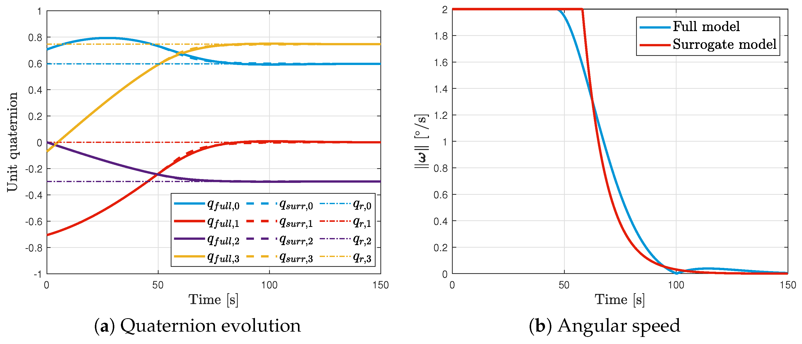
\begin{matrix} {\bar{u}}_{k | k + 1}^{r} : = & A (q (\frac{t_{k} + t_{k + 1}}{2})) u_{k | k + 1}^{b}, \\ u_{k | k + 1}^{b} : = & {[\begin{matrix} 0 & 0 & u_{k} \end{matrix}]}^{⊺} . \end{matrix}

(22)

The attitude kinematics (10) are discretized through a symbolic Runge-Kutta

4^{th}

-order scheme and the discrete kinematics are imposed as constraint (17) in Problem 1. Moreover, the discrete angular velocity vector in constraint (19) in Problem 1,

ω_{k}

, could be obtained by applying formula (9) using the discrete unit quaternion signal,

q_{k}

. It is also worth noting that the squared norms (

{∥q_{k}∥}^{2}

{∥ω_{k}∥}^{2}

, and

{∥q_{r} (t_{k})∥}^{2}

) are constrained instead of the norms themselves. This formulation is adopted to facilitate the job of the optimizer since it allows the Jacobian of the constraints to be defined at all values of

S

and

U

The cost function components of Problem 1,

J_{δ α}

J_{u}

, and

J_{δ q}

are defined as,

\begin{matrix} J_{δ α} & = {(δ α_{n_{p}} - δ α_{r})}^{⊺} P (δ α_{n_{p}} - δ α_{r}) \\ + \sum_{k = 0}^{n_{p} - 1} {(δ α_{k} - δ α_{r})}^{⊺} Q (δ α_{k} - δ α_{r}), \\ J_{u} & = R_{u} \sum_{k = 0}^{n_{u} - 1} u_{k}^{2}, \\ J_{δ q} & = R_{δ q} \sum_{k = 0}^{n_{u} - 1} {δ q_{k}}^{⊺} δ q_{k}, δ q_{k} : = q_{r} (t_{k}) - q (t_{k}), \end{matrix}

(23)

where

δ α_{r}

is the reference ROE vector, while

P \in R^{6 \times 6}

Q \in R^{6 \times 6}

R_{u} \in R^{1}

, and

R_{δ q} \in R^{1}

are positive-definite MPC gains.

It is important to note that the ultimate goal of autonomous orbit keeping is to rendezvous with a virtual target then track its absolute orbit, i.e.

δ α_{r} = 0

. Moreover, the matrices

P

and

Q

are chosen to be diagonal matrices, which renders

J_{δ α}

a summation over the squared weighted 2-norms of the error vector,

δ α_{k} - δ α_{r}

. This ultimately means that

J_{δ α}

is a measure of distance between

δ α_{k}

and

δ α_{r}

, which is zero in our case, in a scaled-ROE space. Indeed, reasoning

J_{δ α}

in terms of the magnitude of the error vector in a scaled-ROE space does not only allow to eventually drive

δ α

δ α_{r}

, and hence for the satellite to rendezvous and then track the orbit of the virtual target, but also allows to indirectly minimize the total delta-V cost, since the distance in the ROE space, or in a scaled-ROE space for that matter (e.g. the dimensional ROE space, which scales the ROE vector by the mean semi-major axis of the chief), can be used as a measure for the total delta-V cost [12,13]. A closer look at

J_{δ α}

reveals that while minimizing it indeed drives the error signal to zero, it is, in fact, an implicit trade-off between fuel and time optimality, depending on the ratio between the traces of

P

and

Q

respectively. The greater the value of this ratio, the more inclined towards fuel-optimality the cost-function becomes, while the lower the ratio, the more the scheme leans towards time-optimality.

Adding

J_{u}

to the compound cost function is set to directly minimize the total required thrust from the onboard single thruster. The adopted convex form of

J_{u}

is the fuel-optimal form of a cost function, which also coincides with the delta-V-optimal form for single-thruster satellites [20].

Finally, the purpose of adding the last component of the cost function,

J_{δ q}

, is to softly constraint the desired attitude to be as close as possible to the actual attitude in order to avoid unnecessary large slews, which in-turn minimizes the attitude control effort. This soft constraint allows large slew maneuvers, depending on the choice of the MPC gains, only when it is meaningful from the ROE error (i.e.

J_{δ α}

) or fuel cost (i.e.

J_{u}

) points of view.

3.2. Parameters tuning

In the proposed formulation of MPC there are many parameters and gains to be chosen, which can affect the overall performance and robustness of the MPC. In many industrial applications the choice of such parameters is done by engineering experience. In this application, the initial guess for the prediction horizon has been formulated based on the literature review. Since the

Δ V

-optimal locations for ROE changes through impulsive delta-V increments are known to occur, at most, every half-orbit [13], and since the input acceleration of the low-thrust propulsion system should be distributed around these

Δ V

-optimal locations (if

Δ V

optimality is sought), the prediction horizon,

n_{p} T_{s}

, is chosen to be at least half the orbital period. In this setting, the MPC is able to foresee all the

Δ V

-optimal locations throughout a certain orbit, which hence leads to optimal allocation of the available thrust. Overly increasing the prediction horizon is expected to only overwhelm the onboard processor, while not having much effect on the optimality of the solution.

The choice of the control horizon,

n_{u} T_{s}

, on the other hand, is done by trial and error, which is an iterative process as all the other parameters have to be fixed before the tuning process starts. Nonetheless, regarding the choice of the

n_{u}

value, it has to be a small positive integer less than or equal to

n_{p}

. Common guidelines for choosing the prediction and control horizons could be found in [21].

Tuning of the sampling time,

T_{s}

, has also been performed by trial and error. In the context of Problem 1, although the dynamics of the ROE are slow and the sampling time could be chosen a large value in order to not solve the optimization problem so frequently, the following important consideration has to be taken into account to carry out the tuning process. Since the attitude dynamics are much faster than that of the ROE, one could not ignore that a fixed value for the input acceleration vector in the RTN frame,

{\bar{u}}_{k | k + 1}^{r}

, is fed to the linearized ROE dynamics constraint (16), see (22), which renders the model used in the MPC not accurate unless a small value of the sampling time is chosen. Indeed, Including

J_{δ q}

in the compound cost function helps in slowing down the attitude dynamics. Still, the need to choose a scant value for the sampling time is meaningful. A compromise had to be done between choosing a small

T_{s}

and have a more accurate model for the MPC on one hand, and choosing a large

T_{s}

which allows the optimization problem to be solved less frequently on the other.

The cost function gains (i.e.

P

Q

R_{u}

, and

R_{δ q}

in this paper) are more challenging to be tuned, since the cost function of the MPC is problem dependent and no general guidelines exist for its weighting. Thus, more focus is put on analyzing the effect of choosing different cost function weights and on actually selecting an optimal set of these weights.

In order to reduce the number of tunable parameters, the component of the cost function, i.e.

J_{δ α}

J_{u}

, and

J_{δ q}

, are related to the main weighting matrix,

Q

, such that,

\begin{matrix} P & = f_{P} Q, \\ {\bar{J}}_{u} & = f_{u} {\bar{J}}_{δ α}, \\ {\bar{J}}_{δ q} & = f_{δ q} {\bar{J}}_{δ α}, \end{matrix}

(24)

where

\begin{matrix} {\bar{J}}_{δ α} : = & (n_{p} + f_{P}) {\bar{δ α}}^{⊺} Q \bar{δ α}, \\ {\bar{J}}_{u} : = & n_{u} R_{u} {\bar{u}}^{2}, \\ {\bar{J}}_{δ q} : = & N_{N} R_{δ q} {\bar{δ q}}^{⊺} \bar{δ q}, \end{matrix}

(25)

with

\bar{δ α}

being the expected value of

δ α

over the prediction horizon, which is approximated by the ROE vector at the beginning of each horizon, and

\bar{u} \approx 0.5 u_{m a x}

and

\bar{δ q} \approx {[\begin{matrix} 0.1 & 0.1 & 0.1 & 0.1 \end{matrix}]}^{⊺}

are predictions for the values of u and

δ q

over the control horizon. The approximated expected values,

\bar{δ α}

\bar{u}

, and

\bar{δ q}

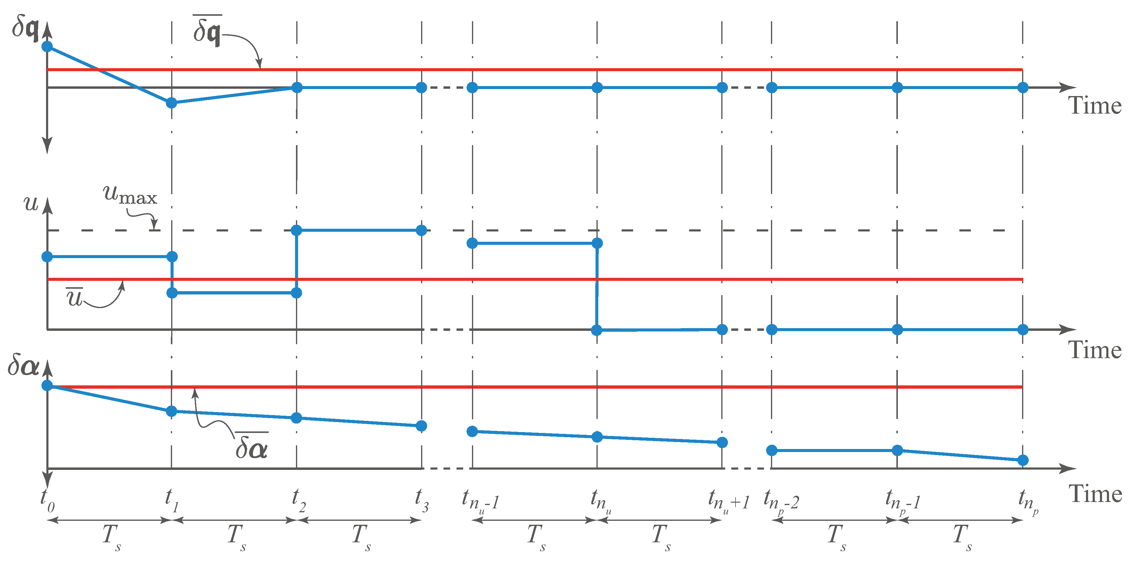
, are illustrated graphically over one prediction horizon in Figure 3. For imaging purposes, each of them is taken one dimensional. Indeed, the values assumed for

\bar{u}

and

\bar{δ q}

are merely the authors’ predictions for the expected values of these quantities over the whole simulation, however, choosing other values for these variables shall not affect the final MPC gains as will be elaborated upon later in the text.

Substituting from (25) into (24), the MPC gains can be related to

Q

\bar{δ α}

\bar{u}

, and

\bar{δ q}

as,

\begin{matrix} R_{u} & = \frac{f_{u} (n_{p} + f_{P})}{n_{u} {\bar{u}}^{2}} {\bar{δ α}}^{⊺} Q \bar{δ α}, \\ R_{δ q} & = \frac{f_{δ q} (n_{p} + f_{P})}{n_{u} {\bar{δ q}}^{⊺} \bar{δ q}} {\bar{δ α}}^{⊺} Q \bar{δ α}, \end{matrix}

(26)

where

R_{u}

and

R_{δ q}

change for every prediction horizon.

It is conceivable that when

δ α : = ∥δ α∥

is very small (i.e. the rendezvous of the satellite with its virtual target has already taken place), the priority should be given to

J_{δ q}

in order for the ADCS not to hyper-react to the small errors in

δ α

. Indeed, the phenomenon of hyper-reaction of the ADCS when

δ α

gets too small has been verified by numerical simulation for a system which is using the definition of

R_{δ q}

in (26). It is for this reason that

R_{δ q}

had to be redefined in order to steer the priority to

J_{δ q}

when

δ α

is approaching zero, such that,

R_{δ q} = Sat (\frac{f_{δ q} (n_{p} + f_{P})}{n_{u} {\bar{δ q}}^{⊺} \bar{δ q}} {\bar{δ α}}^{⊺} Q \bar{δ α}, {R_{δ q}}_{m i n}, \infty),

(27)

where

Sat (x, x_{m i n}, x_{m a x})

is the saturation function which is defined as follows,

Sat (x, x_{m i n}, x_{m a x}) : = \{\begin{matrix} x_{m i n}, & x \leq x_{m i n} \\ x, & x_{m i n} \leq x \leq x_{m a x} \\ x_{m a x}, & x \geq x_{m a x} \end{matrix} .

(28)

Looking at equations (24), (25), (26), and (27), it is clear that in order to define all the MPC gains, one has to choose

Q

f_{P}

f_{u}

f_{δ q}

, and

{R_{δ q}}_{m i n}

The choice of

Q

is rather simple since all the ROE can be weighted equally. However, in order to enhance the stability of the final relative orbit (i.e. to keep the obtained orbit for as long as possible without being much affected by the perturbations), an emphasis is put on minimizing

δ a

when the ROE are close to the target ones, and

Q

is defined as,

Q = \{\begin{matrix} Q I_{6}, & a δ α \leq 1 m \\ Q [\begin{matrix} 100 & 0 \\ 0 & I_{5} \end{matrix}], & a_{c} δ α > 1 m \end{matrix},

(29)

where Q is a tuning parameter that controls the order of magnitude of the cost function, and

I_{n}

is the identity matrix with dimensions

n \times n

Fixing the value of Q to

10^{5}

, of

f_{P}

to 10, and of

{R_{δ q}}_{m i n}

10^{- 5}

, a brute force sensitivity analysis over

f_{u}

and

f_{δ q}

is carried out to choose adroit values for

f_{u}

and

f_{δ q}

. Thanks to the High Performance Computer of the University of Luxembourg [22], 726 simulations could be run simultaneously where in addition to interchanging the values of

f_{u}

and

f_{δ q}

, also the seed of the Random Number Generator (RNG), which controls the initial state at the beginning of the simulation, is taken into account. In these simulations, and in the sequel, warm-starting is employed at the beginning of each prediction horizon, meaning that the optimized state and control profiles from the previous prediction horizon are utilized to construct the initial guess for the current one.

Before starting the simulations, it has been noted that the admissible values for

f_{u}

and

f_{δ q}

belong to the period

[0, 1]

since the most important component of the cost function is

J_{δ α}

and since the two other components are normalized with respect to

J_{δ α}

(see (24)).

One simulation would have its RNG seed,

f_{u}

, and

f_{δ q}

as one possible combination from the following sets,

\begin{matrix} seed \in \{0, 1, 2, 3, 4, 5\}, \\ f_{u}, f_{δ q} \in \{0, 0.02, 0.04, 0.06, 0.08, 0.1, 0.3, 0.6, 0.7, 0.9, 1\}, \end{matrix}

(30)

To this end, a fitness function needs to be introduced in order to asses how good the output of a simulation is. Such fitness function in our context needed to address four criteria (performance metrics),

Driving the ROE vector to zero, which is the main goal of the MPC scheme to achieve orbit keeping. This is assessed through observing the norm of the finale of the ROE time series, denoted as $δ α_{fin}$ .
Enhancing the stability of the relative orbit finale which, in other words, is minimizing the Root-Mean-Square (RMS) of the last portion of the relative semi-major axis profile over time, denoted as $δ a_{fin}$ .
Minimizing the total delta-V, $Δ V_{tot}$ .
Reducing the attitude effort, which is quantified through the mean angular rate of the satellite, ${∥ω∥}_{mean}$ .

It is necessary to state that the term "finale" in this paper refers to the last

10 %

of the simulation time span. Furthermore, although this research is concerned with low-thrust propellers, the total delta-V is considered instead of the total thrust in order to enable comparisons between the proposed scheme and those from the literature. The total delta-V in our context can be calculated using the following formula,

Δ V_{tot} = \int_{t_{init}}^{t_{f i n}} u d t,

(31)

where

t_{init}

and

t_{f i n}

are the initial and final times of the simulation respectively. Given that the input thrust/acceleration from the single thruster is piece-wise constant, the total delta-V can be rewritten as follows,

Δ V_{tot} = \sum_{i = 1}^{n_{h}} {(\sum_{k = 0}^{n_{u} - 1} u_{k} T_{s})}_{j},

(32)

with

n_{h}

being the number of receding horizons being processed within a simulation, j is the horizon index, and

T_{s}

being the fixed sampling time.

The adopted overall fitness function could be then written as,

\begin{matrix} ϕ = K_{δ α} \cdot \underset{ϕ_{δ α}}{\underset{︸}{fitness (δ α_{fin})}} + K_{δ a} \cdot \underset{ϕ_{δ a}}{\underset{︸}{fitness (δ a_{fin})}} \\ + K_{Δ V} \cdot \underset{ϕ_{Δ V}}{\underset{︸}{fitness (Δ V_{tot})}} + K_{∥ω∥} \cdot \underset{ϕ_{∥ω∥}}{\underset{︸}{fitness ({∥ω∥}_{mean})}}, \end{matrix}

(33)

where

K_{δ a}

K_{δ α}

K_{Δ V}

, and

K_{∥ω∥}

are weights that determine the importance of each of the four criterion, and the function

fitness (\cdot)

is defined as,

fitness (x) = \frac{1 / x - min (1 / x)}{max (1 / x) - min (1 / x)},

(34)

with

min (\cdot)

and

max (\cdot)

being the minimum and maximum functions over all the simulations. It is clear the this form of the fitness function only shoots out values between 0 and 1.

Running the simulations for the 726 combinations in (30) for a fixed chief’s initial orbit, defined in Table 1, applying the definition of the fitness function in (34) to all the 726 simulations and to the four performance metrics, and fixing the values of the weights to

K_{δ α} = 5

K_{δ a} = 1

K_{Δ V} = 1

, and

K_{∥ω∥} = 1

, which reflects the high importance of minimizing

δ α_{fin}

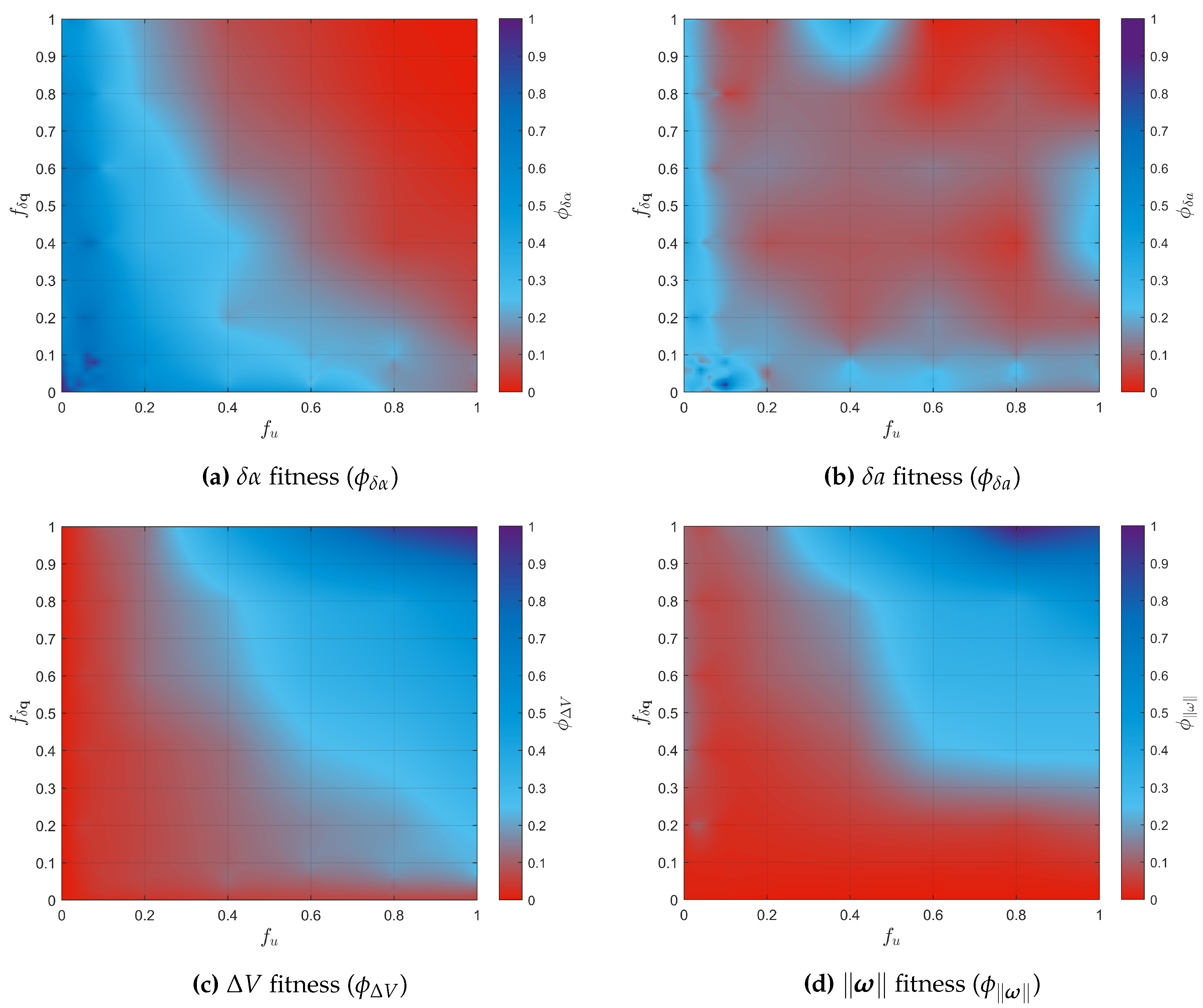
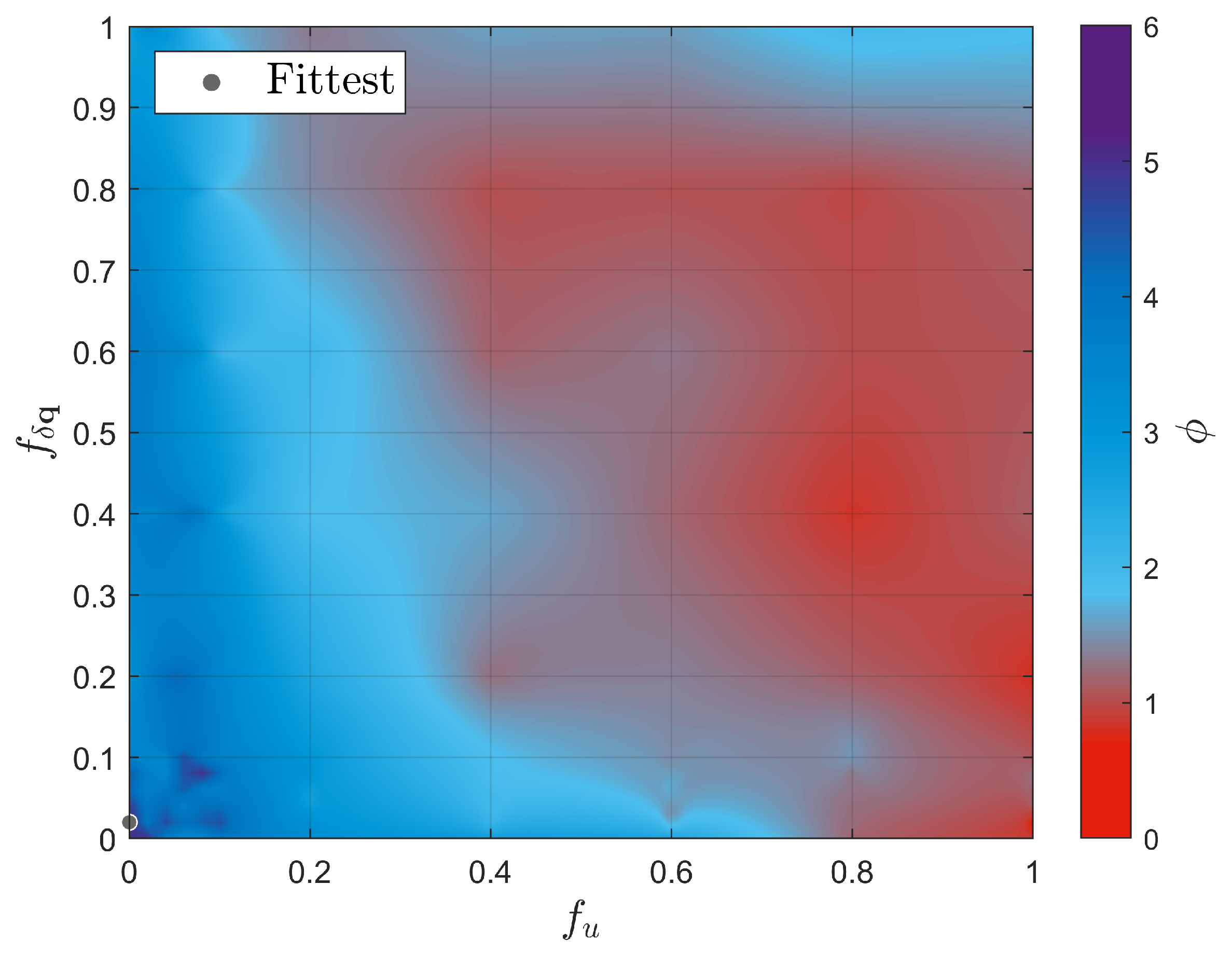
in comparison to the other metrics, the heat maps which summarize all the simulations could be obtained and are presented in Figure 4.

The heat maps in Figure 4 could only be obtained after averaging the fitness over each RNG seed in (30), and after adopting a scattered data interpolant in order to smoothen the heat maps.

It is clear from the figures that the smaller

f_{u}

is, the better

ϕ_{δ α}

and

ϕ_{δ a}

become, while this relation is conceivably inverted for

ϕ_{Δ V}

. Furthermore,

ϕ_{Δ V}

and

ϕ_{∥ω∥}

could be noticed to be positively correlated, and are both negatively correlated with

ϕ_{δ α}

and

ϕ_{δ a}

. Further investigations on the simulations where

ϕ_{Δ V}

and

ϕ_{∥ω∥}

are both large revealed that minimal input acceleration is provided at the current attitude of the satellite which is almost stagnant, while the effect of this acceleration on the orbit correction is, as well, minimal. Nonetheless, the ROE vector is approaching its set point although very slowly.

The overall fitness function,

ϕ

, is depicted in Figure 5 and the fittest point, i.e. the point with maximum overall fitness, (

f_{u} = 0

and

f_{δ q} = 0.02

) is marked with the gray circle on the heat map. It is clear from the fittest

f_{u}

f_{δ q}

combination that, for the initial chief orbit in Table 1, it was not necessary to include the direct delta-V penalty,

J_{u}

, in the cost function, since

J_{δ α}

was already indirectly accounting for delta-V cost as previously mentioned. One has to acknowledge that the fittest combination of

f_{u}

and

f_{δ q}

in Figure 5 is not necessarily universal for any arbitrary initial chief’s orbit, and the selection of the optimal

f_{u}

f_{δ q}

combination needs to be redone for each initial orbit of the virtual chief. This does not represent a limitation of the approach, since the reference orbit of the chief is fixed once as soon as the scientific mission is designed.

The employed approach served the need to identify an adroit set of combination of

f_{u}

and

f_{δ q}

. Future investigations may focus on the set up of a heuristic approach, e.g. genetic algorithms, to search for the combination that globally maximizes the overall fitness function. In this context, note that the definition of the fitness functions and of the related parameters impact the global optimum.

Finally, the values of the optimized

f_{u}

and

f_{δ q}

are heavily dependant on the authors’ prediction for

\bar{u}

and

\bar{δ q}

, and another choice of these quantities would have definitely led to different optimal

f_{u}

and

f_{δ q}

, however, the values of

R_{u}

and

R_{δ q}

will not change since

f_{u}

is directly divided by

{\bar{u}}^{2}

to obtain

R_{u}

and the same dynamics apply for

f_{δ q}

with the squared 2-norm of

\bar{δ q}

to obtain

R_{δ q}

( see (26)).

3.3. Closing the control loop

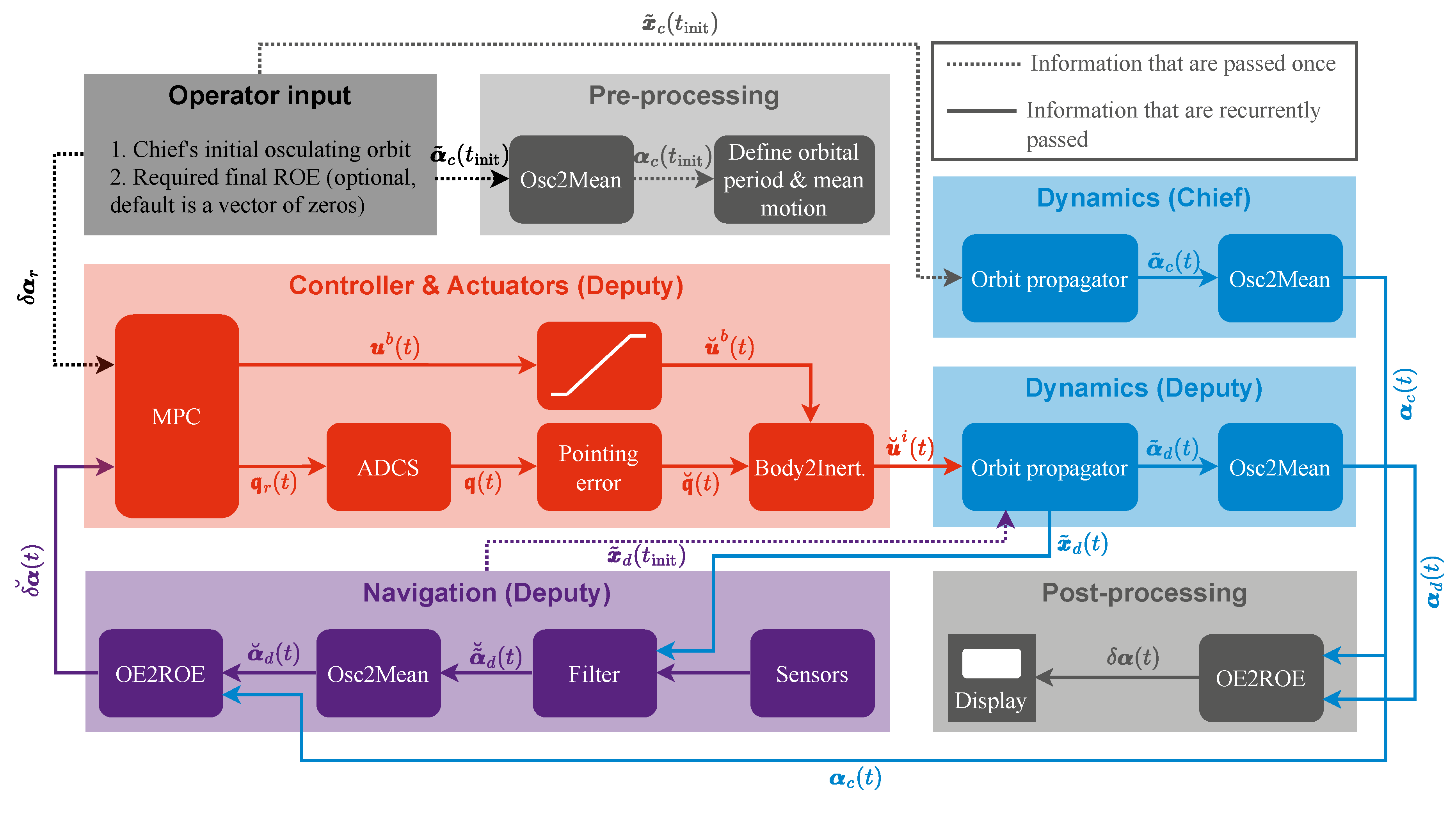
The MPC described so far is one key module of the whole control loop, which, at practical implementation, requires feedback to operate properly, that is provided by the navigation system, which in-turn relies on sensors as well as a state estimation filter. The full closed loop, which illustrates the module execution logic onboard of the deputy spacecraft, is depicted in Figure 6. There, Osc2Mean is the function that transforms osculating orbital elements to mean ones [15], Body2Inert is the method that rotates any vector from the body frame to the inertial frame, and OE2ROE is the function that transforms the absolute orbital elements of both the chief and the deputy to a ROE vector (see (2)). The breve accent,

\overset{˘}{(\cdot)}

, signifies a quantity which is affected by either one or a combination of the following sources of errors:

Estimation errors (e.g. ${\overset{˘}{α}}_{d}$ )
Actuator errors (e.g. $\overset{˘}{q}$ )
Physical constraints (e.g. ${\overset{˘}{u}}^{b}$ )

The proposed MPC is validated by meas of numerical simulations, emulating the performance of the navigation module and the effects of the physical limitations of the adopted actuators.

The physical limitations are only present in the saturation block (see Figure 6) which could be implemented in the numerical simulations. In fact, this saturation is taken into account in the MPC implementation, but the saturation block after the MPC is implemented anyway as a safeguard in case the MPC computes an infeasible solution.

The "Sensors" and "Filter" blocks in Figure 6 are replaced by the following surrogate models which treat the propagated state of the deputy as ground truth,

\begin{matrix} {\overset{˘}{\tilde{x}}}_{d}^{i} = {\tilde{x}}_{d}^{i} + N (0, Σ_{\tilde{x}}), \\ {\overset{˘}{\tilde{α}}}_{d} = Cart 2 OE ({\overset{˘}{\tilde{x}}}_{d}^{i}); \end{matrix}

(35)

where "Cart2OE" is the method that transforms the Cartesian state to orbital elements, and

N (μ, σ^{2})

is a normally distributed random variable with

μ

as its expected value and

σ^{2}

as its variance. Hence,

Σ_{\tilde{x}}

is the covariance matrix of the random noise affecting the estimation of the Cartesian state of the deputy satellite, which is defined as,

Σ_{\tilde{x}} = [\begin{matrix} σ_{r}^{2} & 0 & 0 & 0 & 0 & 0 \\ 0 & σ_{r}^{2} & 0 & 0 & 0 & 0 \\ 0 & 0 & σ_{r}^{2} & 0 & 0 & 0 \\ 0 & 0 & 0 & σ_{v}^{2} & 0 & 0 \\ 0 & 0 & 0 & 0 & σ_{v}^{2} & 0 \\ 0 & 0 & 0 & 0 & 0 & σ_{v}^{2} \end{matrix}],

(36)

where

σ_{r}^{2}

and

σ_{v}^{2}

are the variances of the 1-dimensional position and velocity estimation errors respectively, which, for the numerical simulations presented in this work, is extracted from the publicly available Triton-X brochure.

It is to be noted that the relative navigation is typically more accurate than the absolute one [23,24]. It is for this reason that a similar model is used to emulate the behaviour of the relative navigation system within the numerical simulations as follows,

\begin{matrix} δ α = OE 2 ROE (α_{c}, α_{d}) \\ \overset{˘}{δ α} = δ α + N (0, Σ_{δ α}), \end{matrix}

(37)

where

Σ_{δ α}

is the covariance matrix of the random noise affecting the estimation of the ROE vector, which is expanded as,

Σ_{δ α} = [\begin{matrix} σ_{δ a}^{2} & 0 & 0 & 0 & 0 & 0 \\ 0 & σ_{δ λ}^{2} & 0 & 0 & 0 & 0 \\ 0 & 0 & σ_{δ e_{x}}^{2} & 0 & 0 & 0 \\ 0 & 0 & 0 & σ_{δ e_{y}}^{2} & 0 & 0 \\ 0 & 0 & 0 & 0 & σ_{δ i_{x}}^{2} & 0 \\ 0 & 0 & 0 & 0 & 0 & σ_{δ i_{y}}^{2} \end{matrix}],

(38)

with the diagonal elements being the variances of the random noise that affect each element of the ROE vector. These variances are taken to be all equal in the sequel, i.e.

σ_{δ a} = σ_{δ λ} = σ_{δ e_{x}} = σ_{δ e_{y}} = σ_{δ i_{x}} = σ_{δ i_{y}} = σ_{δ α}

Lastly, the "Pointing error" block is replaced by the following surrogate model,

\begin{matrix} \overset{˘}{q} = q \circ q_{pe}, \\ q_{pe} = {[\begin{matrix} cos (\frac{ζ_{q_{pe}}}{2}) & sin (\frac{ζ_{q_{pe}}}{2}) {\hat{q}}_{pe}^{⊺} \end{matrix}]}^{⊺}, \end{matrix}

(39)

where

ζ_{q_{pe}}

is the pointing error angle, which is obtained from Triton-X brochure in the validation simulations, and

{\hat{q}}_{pe}

is a random 3-element unit vector.

It is important to note that although the chief, in this context, is a virtual point, it is propagated using the perturbed dynamics for two main reasons,

in many applications the tracking of the reference orbit and the absolute control of the reference orbit are handled separately;
the proposed scheme can be directly applied to the rendezvous to an actual spacecraft.

As a result, the autonomous orbit keeping compensates errors and perturbations acting on the relative dynamics.

4. MPC validation

In order to test the stability of the proposed MPC scheme, and thanks to the parallelization capabilities of the HPC facilities of the University of Luxembourg, the algorithm was run over 500 different simulations, each with a different initial ROE vector such that,

a_{c} \cdot δ α (t_{init}) [m] \in [\begin{matrix} [- 100, 100] \\ [- 1000, 1000] \\ [- 100, 100] \\ [- 100, 100] \\ [- 100, 100] \\ [- 100, 100] \end{matrix}],

(40)

where

t_{init}

is the initial time of each simulation.

The simulation and MPC parameters used in the 500-run Monte-Carlo simulation are summarized in Table 2.

It is to be noted that although the sampling time used in predicting the MPC states,

T_{s}

, is 50 s, the attitude dynamics are propagated each second in the simulations since the attitude changes much faster than the ROE. Moreover, constraining the maximum allowable acceleration is a consequence of the physical constraint on the maximum thrust that can be provided by the onboard throttleable electric propulsion system. The value of the maximum allowable acceleration,

u_{m a x}

, is obtained for the following simulations from the information on Triton-X brochure on both, the maximum thrust, which is set equal to 7 mN, and the mass of the satellite, which is assumed to be constant, 200 kg, throughout the maneuver.

The main performance metrics over the 500 Monte-Carlo runs are depicted in Figure 7, while the statistics of these metrics are presented in Table 3.

In order to gain an insight on how the proposed scheme performs, the results of an arbitrary simulation out of the 500 simulations are presented. The randomly selected initial ROE (according to (40)) vector is given in Table 4 alongside the reference ROE vector.

The ROE states are seen to approach their set points (zeros for rendezvous with the virtual target) in Figure 8. It is of significance to mention that the chief’s mean orbital period, which is the unit of time in Figure 8, counts to

5974.46

seconds.

The trajectory followed by the satellite is depicted in Figure 9 in both, the Transversal-Radial and the Normal-Radial planes. This trajectory could be obtained by transforming the ROE to the relative Cartesian states in the RTN frame using the transformation in [25]. It can be seen from Figure 9 that the orbit maneuver is taking place gradually thanks to the continuous firing of the thruster, in contrast to the impulsive-thrust maneuvers where the velocity changes at a handful of points on the orbit.

The thrust exerted by the onboard thruster is depicted in Figure 10. This thrust is also projected on the RTN frame and the projection is presented on the same figure. It is interesting to see that the MPC does not follow a trajectory which minimizes the radial burns, which is a usual constraint imposed on the MPC in earlier researches [14]. Although firing in the radial direction to correct

δ λ

errors is known to be more delta-V expensive than firing in the Transversal direction to build up

δ a

drift which takes care of correcting the

δ λ

error by exploiting the natural dynamics, this is not the case for close proximity maneuvers where the initial

δ λ

error is small. This can be verified by looking at the solution to the linearized forced Gauss variational equations [16], and it could also be verified by our preliminary experiments in which the projection of thrust on the radial direction was soft-constrained.

In Figure 11a, the error quaternion angle signal suggests that at each optimization step, the attitude starts from a value which does not coincide with the reference attitude. Nevertheless, by the end of each step, the attitude gradually converges towards the reference one, resulting in the error quaternion angle approaching a value close to zero. A very interesting feature of the proposed scheme is that the propulsion system is always turned on even when attitude redirection maneuvers are taking place. The optimizer calculates the reference attitude knowing that the satellite will not necessarily be aligned with it for the whole upcoming control step.

It is worth noting that the angle of any quaternion (e.g. the error quaternion,

q_{e}

or the current quaternion,

q

) can be found as,

ζ_{q} = arctan (\frac{∥q∥}{q_{0}}),

(41)

where

∥q∥

and

q_{0}

are the vector and the scalar parts of the quaternion

q

respectively. Lastly, the effect of adding the

J_{δ q}

term to the cost function of Problem 1 could be seen clearly in Figure 11 where the quaternion angle rate is depicted. The quaternion angle rate, which can be thought of as a signed version of

∥ω∥

, is seen in to be much less than its maximum allowable values,

2^{\circ} / s

. Our preliminary simulations which did not contain the term

J_{δ q}

on their cost function always had the attitude rate saturating at its maximum value, which is a hyper-reaction that is not desired in a real mission.

In order to test the efficiency and the optimality of the proposed MPC scheme, it is benchmarked against the approach proposed in [14] for a similar problem, where an out-of-plane (OOP) relative orbit correction maneuver had to be performed. The parameters used for this benchmark simulation are summarized in Table 5. Any missing parameter in Table 5 is set to its value in Table 2 except for the maximum allowable acceleration which is set to

u_{m a x} = 3.2 \cdot 10^{- 5} m / s^{2}

. Applying this maximum acceleration to the satellite employed in [14], which has a mass of 20 kg, renders the maximum thrust to be

0.64

mN.

The setting of this maneuver is interesting not only because it allows comparing two different MPC schemes, but also because OOP maneuvers require only normal acceleration. In fact, the

Δ V

-optimal locations for impulsive normal burns for such maneuvers could be analytically calculated [13]. For the case of electric propulsion, a controller is said to be

Δ V

-optimal for out-of-plane maneuvers if the thrust in the normal direction is bang-bang-like and is distributed almost evenly around the

Δ V

-optimal locations. The thrust profile of the proposed MPC is depicted in Figure 12, which reveals that the proposed MPC behaves as a fuel-efficient scheme would be expected to behave.

It could also be seen from Figure 12 that the thrust components in the radial and the transversal directions are not exactly zero due to in-plane perturbation compensation and also owing to the fact that the thrust is provided during slew maneuvers. Therefore the radial and transversal thrust components become more visible when the thrust direction is required to flip from the positive to the negative normal direction. In this situation, the satellite has to pass by many transient attitudes for which the radial and the transversal components are not necessarily zero.

Figure 12 depicts a comparison between the normal component of the thrust profile of the proposed MPC scheme and the MPC scheme proposed by [14].

The dimensional ROE profiles of the two MPCs are also shown in Figure 13, and a brief comparison between the performance of both schemes is presented in Table 6, where the convergence time is defined as the time it takes all elements in the error dimensional ROE vector,

a_{c} δ α_{err} = a_{c} (δ α - δ α_{r})

, to be less than

5 [m]

It is clear from Table 6 as well as Figure 13 that, for the simulation defined by Table 5, the proposed scheme is much faster, in fact,

1.61

times as fast as that of [14]. Furthermore, the proposed MPC appears to be much more precise than the reference one, however, it consumes

24.04 %

more delta-V as seen in Table 6. Indeed, consuming more delta-V than the reference MPC is conceivable since the proposed MPC is not designed to be delta-V-optimal in the first place. Again, the cost function of Problem 1 has two components (after eliminating

J_{u}

as discussed in Section 3.2), the first one,

J_{δ α}

, deals with gradually approaching the reference ROE vector, and implicitly implies a trade-off between fuel and time optimality (depending on

f_{P}

), while the second component,

J_{δ q}

, is added to minimize the attitude change throughout the maneuver. It is believed that a smaller total delta-V could be achieved by a different set of MPC gains, however, it would be at the cost of more abrupt attitude changes and/or more maneuvering time. The ROE profile in Figure 13 implies the evolution of the OOP variables,

δ i_{x}

and

δ i_{y}

, from their initial values to their set points, while the in-plane variables fluctuate slightly around their initial/reference values as a response to the relative orbital perturbations as well as to the unavoidablee radial and transversal accelerations during each attitude flip from the positive to the negative normal direction and vise-versa.

Lastly, Figure 14 relates to the attitude evolution of the system, where Figure 14 shows how the attitude is changing smoothly to recurrently flip the thrust direction from/to the positive to/from the negative normal direction, while the error quaternion angle is starting from a non-zero value only when the thrust direction is required to be flipped, and is seen to always approach zero. Moreover, although the objective is clearly to flip the thrust direction, the error quaternion angle is never

180^{\circ}

, which could only mean that the optimizer chooses the reference quaternion to evolve smoothly until it reaches the flipped attitude so that hyper-reaction of angular velocity could be avoided. The quaternion angle rate is seen in Figure 14 to turn swiftly and reach almost its full potential, i.e.

\pm ω_{m a x}

, when the thrust direction is set to change from/to the positive to/from the negative normal direction.

5. Conclusion

This paper proposes a MPC scheme to address the problem of optimal absolute orbit keeping for under actuated satellites which use electrical propulsion systems. Currently, several small-satellite platforms are equipped with unidirectional thrusters, which requires constant attitude slews to take place during time-extended orbit maneuvers in order to redirect the thruster to the desired propulsion direction. Although the proposed controller is concerning a single satellite, formation flying techniques have been utilized by assuming the satellite to be flying in a formation with a virtual spacecraft (flying on the reference trajectory) with respect to which it is required to keep a predefined relative orbit (rendezvous in most cases). This approach allows leveraging the astrodynamics’ insight into the classical linearized control problem. Moreover, this allows a direct implementation of the proposed algorithm in true multi-satellite relative orbit keeping contexts.

Designed to comprise a trade-off between fuel and time optimality through manipulating the controller gains, the proposed MPC couples the attitude and the relative orbital dynamics such that the control thrust is provided during the attitude redirection maneuvers. The stability of the control scheme is verified through Monte-Carlo numerical simulations in which navigation errors, hardware errors, and physical constraints are emulated. In order to assess the controller’s performance, the proposed MPC has also been compared to a reference MPC from the literature. As for the compared scenario, the proposed MPC achieves a more accurate orbit keeping in a shorter time frame. Such outperforming is achieved at the cost of a slightly larger delta-v cost, corresponding to approximately the 24% of the total maneuver cost, and therefore negligible at mission level.

Acknowledgments

This research was funded in whole, or in part, by the Luxembourg National Research Fund (FNR), grant reference BRIDGES/19/MS/14302465. For the purpose of open access, and in fulfilment of the obligations arising from the grant agreement, the author has applied a Creative Commons Attribution 4.0 International (CC BY 4.0) license to any Author Accepted Manuscript version arising from this submission.

The experiments presented in this paper were carried out using the HPC facilities of the University of Luxembourg [22].

Appendix A. Stability of the surrogate model of the ADCS

Letting

q_{e}

be the unit error quaternion between the desired and the actual attitudes, and

ω_{e} : = ω - ω_{r}

be the error angular velocity vector, with

ω

being the angular velocity vector and

ω_{r}

being the reference/set point of

ω

, the dynamics of the error unit quaternion as given by [18] could be written as,

{\dot{q}}_{e} = \frac{1}{2} q_{e} \circ ω_{e} .

(A1)

Note that, for slew maneuvers, the reference angular velocity vector is always zero, i.e.

ω_{r} = 0

, which enables (A1) to be rewritten as,

{\dot{q}}_{e} = \frac{1}{2} q_{e} \circ ω .

(A2)

If the angular velocity profile could be forced, via the input torques, to follow (9), i.e.

ω = - K q_{e, 0} q_{e}

, the error quaternion kinematics could be expressed as,

{\dot{q}}_{e} = - \frac{K q_{e, 0}}{2} q_{e} \circ q_{e} = - \frac{K q_{e, 0}}{2} [\begin{matrix} - {∥q_{e}∥}^{2} \\ q_{e, 0} q_{e} \end{matrix}] = \frac{K}{2} [\begin{matrix} {∥q_{e}∥}^{2} q_{e, 0} \\ - q_{e, 0}^{2} q_{e} \end{matrix}] .

(A3)

Noting that K is a positive gain, (A3) could be rewritten as,

[\begin{matrix} {\dot{q}}_{e, 0} \\ {\dot{q}}_{e, 1} \\ {\dot{q}}_{e, 2} \\ {\dot{q}}_{e, 3} \end{matrix}] = [\begin{matrix} K_{0} q_{e, 0} \\ - K_{1} q_{e, 1} \\ - K_{2} q_{e, 2} \\ - K_{3} q_{e, 3} \end{matrix}],

(A4)

where

K_{0}

K_{1}

K_{2}

, and

K_{3}

, are all positive, and

q_{e, 1}

q_{e, 2}

, and

q_{e, 3}

are the three components of

q_{e}

. Equation (A4) suggests that, under the constraint

∥q_{e}∥ = 1

, the error quaternion asymptotically approaches either

{[\begin{matrix} 1 & 0 & 0 & 0 \end{matrix}]}^{⊺}

{[\begin{matrix} - 1 & 0 & 0 & 0 \end{matrix}]}^{⊺}

no matter the initial condition of

q_{e}

References

Miller, S.; Walker, M.L.R.; Agolli, J.; Dankanich, J. Survey and Performance Evaluation of Small-Satellite Propulsion Technologies. Journal of Spacecraft and Rockets 2021, 58, 222–231. [Google Scholar] [CrossRef]
Helmeid, E.; Buursink, J.; Poppe, M.; Ries, P.; Gales, M. The Integrated Avionics Unit – performance, innovation and application. Poster presentation at The 4S Symposium, 2022. Vilamoura, Portugal, 2022.
Floberghagen, R.; Fehringer, M.; Lamarre, D.; Muzi, D.; Frommknecht, B.; Steiger, C.; Piñeiro, J.; Da Costa, A. Mission design, operation and exploitation of the gravity field and steady-state ocean circulation explorer mission. Journal of Geodesy 2011, 85, 749–758. [Google Scholar] [CrossRef]
Königsmann, H.J.; Collins, J.T.; Dawson, S.; Wertz, J.R. Autonomous orbit maintenance system. Acta Astronautica 1996, 39, 977–985, IAA International Symposium on Small Satellites for Earth Observation,. [Google Scholar] [CrossRef]
De Florio, S.; D’Amico, S. The precise autonomous orbit keeping experiment on the PRISMA mission. The Journal of the Astronautical Sciences 2008, 56, 477–494. [Google Scholar] [CrossRef]
Garulli, A.; Giannitrapani, A.; Leomanni, M.; Scortecci, F. Autonomous Low-Earth-Orbit Station-Keeping with Electric Propulsion. Journal of Guidance, Control, and Dynamics 2011, 34, 1683–1693. [Google Scholar] [CrossRef]
Bonaventure, F.; Baudry, V.; Sandre, T.; helene Gicquel, A. Autonomous Orbit Control for Routine Station-Keeping on a LEO Mission. In Proceedings of the Proceedings of the 23rd International Symposium on Space Flight Dynamics; 2012. [Google Scholar]
De Florio, S.; D’Amico, S.; Radice, G. Virtual Formation Method for Precise Autonomous Absolute Orbit Control. Journal of Guidance, Control, and Dynamics 2014, 37, 425–438. [Google Scholar] [CrossRef]
Steindorf, L.M.; D’Amico, S.; Scharnagl, J.; Kempf, F.; Schilling, K. Constrained low-thrust satellite formation-flying using relative orbit elements. In Proceedings of the 27th AAS/AIAA Space Flight Mechanics Meeting; 2017; Vol. 160, pp. 3563–3583. [Google Scholar]
Silvestrini, S.; Lavagna, M. Neural-aided GNC reconfiguration algorithm for distributed space system: development and PIL test. Advances in Space Research 2021, 67, 1490–1505. [Google Scholar] [CrossRef]
Gaias, G.; Ardaens, J.S. Flight Demonstration of Autonomous Noncooperative Rendezvous in Low Earth Orbit. Journal of Guidance, Control, and Dynamics 2018, 41, 1337–1354. [Google Scholar] [CrossRef]
Gaias, G.; D’Amico, S.; Ardaens, J.S. Generalised multi-impulsive manoeuvres for optimum spacecraft rendezvous in near-circular orbit. International Journal of Space Science and Engineering 2015, 3, 68–88. [Google Scholar] [CrossRef]
Gaias, G.; D’Amico, S. Impulsive Maneuvers for Formation Reconfiguration Using Relative Orbital Elements. Journal of Guidance, Control, and Dynamics 2015, 38, 1036–1049. [Google Scholar] [CrossRef]
Belloni, E.; Silvestrini, S.; Prinetto, J.; Lavagna, M. Relative and absolute on-board optimal formation acquisition and keeping for scientific activities in high-drag low-orbit environment. Advances in Space Research 2023. [Google Scholar] [CrossRef]
Gaias, G.; Colombo, C.; Lara, M. Analytical Framework for Precise Relative Motion in Low Earth Orbits. Journal of Guidance, Control, and Dynamics 2020, 43, 915–927. [Google Scholar] [CrossRef]
Di Mauro, G.; Bevilacqua, R.; Spiller, D.; Sullivan, J.; D’Amico, S. Continuous maneuvers for spacecraft formation flying reconfiguration using relative orbit elements. Acta Astronautica 2018, 153, 311–326. [Google Scholar] [CrossRef]
Sidi, M.J. Spacecraft dynamics and control: a practical engineering approach; Cambridge university press,, 1997; Vol. 7. [Google Scholar] [CrossRef]
Mahfouz, A.; Pritykin, D.; Biggs, J. Hybrid Attitude Control for Nano-Spacecraft: Reaction Wheel Failure and Singularity Handling. Journal of Guidance, Control, and Dynamics 2021, 44, 548–558. [Google Scholar] [CrossRef]
Wie, B.; Weiss, H.; Arapostathis, A. Quaternion feedback regulator for spacecraft eigenaxis rotations. Journal of Guidance, Control, and Dynamics 1989, 12, 375–380. [Google Scholar] [CrossRef]
Ross, I.M. Space Trajectory Optimization and L1-Optimal Control Problems. In Modern Astrodynamics; Gurfil, P., Ed.; Butterworth-Heinemann, 2006; Vol. 1, Elsevier Astrodynamics Series, chapter 6, pp. 155–VIII. [CrossRef]
Alhajeri, M.; Soroush, M. Tuning Guidelines for Model-Predictive Control. Industrial & Engineering Chemistry Research 2020, 59, 4177–4191. [Google Scholar] [CrossRef]
Varrette, S.; Bouvry, P.; Cartiaux, H.; Georgatos, F. Management of an Academic HPC Cluster: The UL Experience. In Proceedings of the Proc. of the 2014 Intl. Conf. on High Performance Computing & Simulation (HPCS 2014); IEEE: Bologna, Italy, 2014; pp. 959–967. [Google Scholar]
Mahfouz, A.; Menzio, D.; Dalla Vedova, F.; Voos, H. Relative State Estimation for LEO Formations with Large Inter-satellite Distances Using Single-Frequency GNSS Receivers. In Proceedings of the Proceedings of the 11th International Workshop on Satellite Constellations & Formation Flying; 2022. [Google Scholar]
Mahfouz, A.; Menzio, D.; Dalla Vedova, F.; Voos, H. GNSS-based baseline vector determination for widely separated cooperative satellites using L1-only receivers. Advances in Space Research 2023. [Google Scholar] [CrossRef]
Gaias, G.; Lovera, M. Trajectory Design for Proximity Operations: The Relative Orbital Elements’ Perspective. Journal of Guidance, Control, and Dynamics 2021, 44, 2294–2302. [Google Scholar] [CrossRef]

1	The brochure can be found through: https://www.ohb.de/fileadmin/artundweise/downloads/Triton-X_Heavy_Specification_and_Description_2021.pdf

Figure 1. Snapshot of the shape of the relative orbit (i.e. orbit drift is neglected).

Figure 2. Validation of the surrogate ADCS model through random initial and desired attitudes.

Figure 3. Assumed expected values,

\bar{δ α}

\bar{u}

, and

\bar{δ q}

over one prediction horizon.

Figure 3. Assumed expected values,

\bar{δ α}

\bar{u}

, and

\bar{δ q}

over one prediction horizon.

Figure 4. Fitness of the four performance metrics.

Figure 5. Overall fitness (

ϕ

Figure 5. Overall fitness (

ϕ

Figure 6. Closed loop of the deputy spacecraft.

Figure 7. Performance metrics over the Monte-Carlo simulation.

Figure 8. ROE profile of the Monte-Carlo run defined by Table 4.

Figure 9. Followed trajectory by the satellite of the Monte-Carlo run defined by Table 4.

Figure 10. Thrust level of the Monte-Carlo run defined by Table 4.

Figure 11. Attitude profile of the Monte-Carlo run defined by Table 4.

Figure 12. Thrust level for the benchmark simulation.

Figure 13. ROE profile of the benchmark maneuver defined by Table 5.

Figure 14. Attitude profile of the benchmark maneuver defined by Table 5.

Table 1. Chief’s initial orbit for all the 726 simulations used in the sensitivity analysis.

${\tilde{a}}_{c}$ [km]	${\tilde{θ}}_{c}$ [^∘]	${{\tilde{e}}_{x}\|}_{c}$	${{\tilde{e}}_{y}\|}_{c}$	${\tilde{i}}_{c}$ [^∘]	${\tilde{Ω}}_{c}$ [^∘]
7121	0	$10^{- 5}$	0	45	0

Table 2. Monte-Carlo simulation and MPC parameters.

Chief’s initial orbit	${\tilde{a}}_{c}$ [km]	${\tilde{θ}}_{c}$ [^∘]	${{\tilde{e}}_{x}\|}_{c}$	${{\tilde{e}}_{y}\|}_{c}$	${\tilde{i}}_{c}$ [^∘]	${\tilde{Ω}}_{c}$ [^∘]
	7121	0	$10^{- 5}$	0	45	0
MPC parameters		$T_{s}$ [s]	$n_{p}$ [ $T_{s}$ ]	$n_{u}$ [ $T_{s}$ ]	$u_{m a x}$ [ $m / s^{2}$ ]	$ω_{m a x}$ [^∘/s]
		50 s	60	15	$3.5 \times 10^{- 5}$	2
		Q	$f_{P}$	$f_{u}$	$f_{δ q}$	$R_{{δ q}_{m i n}}$
		$10^{5}$	10	$0.0$	$0.02$	$10^{- 5}$
Miscellaneous		K	$σ_{r}$ [m]	$σ_{v}$ [ $m / s$ ]	$a_{c} σ_{δ α}$ [m]	$ζ_{q_{pe}}$ [arcs]
		$0.2$	10	0.5	1	25

Table 3. Performance metrics over 500 simulations.

	$a_{c} δ α_{fin}$ [m]	$a_{c} δ a_{fin}$ [m]	$Δ V_{tot}$ [ $m / s$ ]	${∥ω∥}_{mean}$ [^∘/s]
Mean	$4.38$	$2.05$	$0.406$	$0.228$
Median	$4.29$	$2.02$	$0.409$	$0.226$
Max	$9.82$	$4.49$	$0.58$	$0.331$

Table 4. Parameters of an arbitrary simulation out of the 500 Monte-Carlo runs.

Initial ROE	$a_{c} δ a$ [m]	$a_{c} δ λ$ [m]	$a_{c} δ e_{x}$ [m]	$a_{c} δ e_{y}$ [m]	$a_{c} δ i_{x}$ [m]	$a_{c} δ i_{y}$ [m]
	$64.62$	$- 947.77$	$- 57.84$	$23.68$	$- 80.35$	$24.03$
Reference ROE	$a_{c} δ a$ [m]	$a_{c} δ λ$ [m]	$a_{c} δ e_{x}$ [m]	$a_{c} δ e_{y}$ [m]	$a_{c} δ i_{x}$ [m]	$a_{c} δ i_{y}$ [m]
	0	0	0	0	0	0

Table 5. Benchmark simulation parameters.

Chief’s initial orbit	${\tilde{a}}_{c}$ [km]	${\tilde{θ}}_{c}$ [^∘]	${{\tilde{e}}_{x}\|}_{c}$	${{\tilde{e}}_{y}\|}_{c}$	${\tilde{i}}_{c} [^{\circ}]$	${\tilde{Ω}}_{c}$ [^∘]
Chief’s initial orbit	6828	0	$10^{- 5}$	0	78	0
Initial ROE	$a_{c} δ a$ [m]	$a_{c} δ λ$ [m]	$a_{c} δ e_{x}$ [m]	$a_{c} δ e_{y}$ [m]	$a_{c} δ i_{x}$ [m]	$a_{c} δ i_{y}$ [m]
Initial ROE	0	0	273	0	10	70
Reference ROE	$a_{c} δ a$ [m]	$a_{c} δ λ$ [m]	$a_{c} δ e_{x}$ [m]	$a_{c} δ e_{y}$ [m]	$a_{c} δ i_{x}$ [m]	$a_{c} δ i_{y}$ [m]
Reference ROE	0	0	273	0	400	120

Table 6. Comparison between the proposed and the reference MPCs.

	Convergence time [orbits]	Terminal $a_{c} (δ α - δ α_{r}) [m]$	$Δ V_{tot} [m / s]$
Proposed MPC	$4.1$	${[\begin{matrix} 0.9 & - 0.4 & 1.9 & - 0.33 . & 0.0 & - 0.5 \end{matrix}]}^{⊺}$	$0.664$
Reference MPC	$6.6$	${[\begin{matrix} - 3.6 & 9.2 & - 1.4 & 2.0 & - 2.9 & 1.6 \end{matrix}]}^{⊺}$	$0.501$

Disclaimer/Publisher’s Note: The statements, opinions and data contained in all publications are solely those of the individual author(s) and contributor(s) and not of MDPI and/or the editor(s). MDPI and/or the editor(s) disclaim responsibility for any injury to people or property resulting from any ideas, methods, instructions or products referred to in the content.

© 2023 by the authors. Licensee MDPI, Basel, Switzerland. This article is an open access article distributed under the terms and conditions of the Creative Commons Attribution (CC BY) license (https://creativecommons.org/licenses/by/4.0/).

Copyright: This open access article is published under a Creative Commons CC BY 4.0 license, which permit the free download, distribution, and reuse, provided that the author and preprint are cited in any reuse.

MDPI Initiatives

Important Links

Choose an area of interest and we will send you notifications of new preprints at your preferred frequency.

Disclaimer

Autonomous Optimal Absolute Orbit Keeping Through Formation-Flying Techniques

Abstract

1. Introduction

2. Mathematical models

2.1. Relative orbital dynamics

2.2. Attitude kinematics

3. Model-Predictive Control

3.1. MPC problem formulation

3.2. Parameters tuning

3.3. Closing the control loop

4. MPC validation

5. Conclusion

Acknowledgments

Appendix A. Stability of the surrogate model of the ADCS

References

MDPI Initiatives

Important Links

Subscribe