Signal Filtering Using Neuromorphic Measurements

Preprint

Article

Signal Filtering Using Neuromorphic Measurements

Altmetrics

Downloads

Views

Comments

A peer-reviewed article of this preprint also exists.

This version is not peer-reviewed

Submitted:

18 October 2023

Posted:

19 October 2023

You are already at the latest version

Alerts

Abstract

Digital filtering is a fundamental technique in digital signal processing, which operates on a digital sequence without any information on how the sequence was generated. This paper proposes a methodology for designing the equivalent of digital filtering for neuromorphic samples, which are a low power alternative to conventional digital samples. In the literature, filtering using neuromorphic samples is done by filtering the reconstructed analog signal, which is required to belong to a predefined input space. We show that this requirement is not necessary, and introduce a new method for computing the neuromorphic samples of the filter output directly from the input samples, backed by theoretical guarantees. We show numerically we can achieve a similar accuracy compared to the conventional method. However, given that we bypass the analog signal reconstruction step, our results show significantly reduced computation time for the proposed method and good performance even when signal recovery is not possible.

Keywords:

Subject: Engineering - Electrical and Electronic Engineering

1. Introduction

In contemporary computing, the majority of tasks necessitate some form of digital signal processing [1]. With the escalating computational capabilities of digital processing systems, there is a concurrent surge in power consumption. This is further exacerbated by the rapid advancements in the field of artificial intelligence. Neuromorphic sampling, or time encoding, is an alternative to traditional digital encoding that transforms an analog signal into a sequence of low-power time-based pulses, often referred to as a spike train. Neuromorphic sampling draws its inspiration from neuroscience and introduces a paradigm shift by significantly reducing power consumption during encoding and transmission [2,3]. Despite these advantages, as of now, there exists no equivalent of digital signal processing operations tailored to neuromorphic sampling. This unexplored territory holds the promise of groundbreaking developments in low-power and efficient signal processing.

In this paper, we address the problem of filtering a signal using its neuromorphic measurements, thus extending the principle of digital signal filtering for the case of neuromorphic sampling. In the literature, the concept of spike train filtering predominantly refers to convolving the filter function with a sequence of Diracs centered in the spike times [4]. This is not an operation on the analog signal that resulted in those neuromorphic samples. Moreover, in the context of neuromorphic measurements generated from multidimensional signals, such as those generated by event-cameras [5], filtering also refers to performing multidimensional spatial convolution [6,7]. The case of filtering the analog signal via its neuromorphic measurements was proposed in [8], but the process also involves signal reconstruction. A filtering approach of neuromorphic signals without reconstruction was first studied in [9].

Therefore, conventionally, to process the signal underlying a sequence of spike measurements, the signal is recovered in the analog domain, followed by filtering and neuromorphic sampling. There are a number of drawbacks with this approach. First, this method does not exploit the power consumption advantage of neuromorphic measurements. Second, this approach is heavier computationally due to the complexity of signal reconstruction from neuromorphic samples [10,11]. Third, reconstruction is only possible if the input satisfies some restrictive smoothness or sparsity constraints. However, for conventional sampling, the process of digital filtering is independent of the charateristics of the signal that generated the measurements.

In this paper, we derive a direct mapping between the time encoded inputs and outputs of an analog filter. The proposed mapping forms the basis for a practical filtering algorithm of the underlying signal corresponding to some given neuromorphic measurements, without direct access to the signal. We introduce theoretical guarantees and error bounds for the measurements generated with the proposed algorithm. Throrugh numerical simulations, we demonstrate the performance of our method in terms of speed, but also reduced restrictions on the input signal, in comparison with the existing conventional method.

This paper is structured as follows. Section 2 presents a brief review of the time encoding model used in this paper. Section 3 introduces the proposed problem. Section 4 describes the proposed filtering method. Numerical results are in Section 5. Section 6 presents the concluding remarks.

2. Time Encoding

The time encoding machine (TEM) is a conceptualization of neuromorphic sampling that maps an input

u (t)

into a sequence of samples

{t_{k}}_{k \in}

. The particular TEM considered here is the integrate-and-fire (IF) TEM, which is inspired from neuroscience. Consequently, sequence

{t_{k}}_{k \in}

is called a spike train, where the spike refers to the firing of an action potential, representing the information transmission method in the mammalian cortex. Previously, the IF model was used for system identification of biological neurons [12,13], to perform machine learning tasks [14,15] but also for input reconstruction [11,16,17,18,19]. The IF model adds an input

g (t)

with bias parameter b, and subsequently integrates the output to generate a strictly increasing function

y (t)

. When

y (t)

crosses threshold

δ

, the integrator is reset and the IF generates an output spike time

t_{k}

. The IF TEM is described by the following equations

\int_{t_{k}}^{t_{k + 1}} u (s) d s = δ - b t_{k + 1} - t_{k}, k \in_{+}^{*} .

(1)

Without reducing the generality, it is assumed that

t_{0} = 0

. A common assumption is that the input is bounded by

c \in_{+}

, such that

u (t) \leq c < b

. This bound enables deriving the following density guarantees [2]

\frac{δ}{b + c} \leq t_{k + 1} - t_{k} \leq \frac{δ}{b - c} .

(2)

Signal

u (t)

is, in the general case, not recoverable from

{\{t_{k}\}}_{k \in Z}

. To ensure it can be reconstructed, we require imposing restrictive assumptions. A common assumption is that

u (t)

belongs to

P W_{Ω}

, the space of functions bandlimited to

Ω rad / s

that are also square integrable, i.e.,

u \in L^{2}

. If this assumption is satisfied, then

u (t)

can be recovered from

{\{t_{k}\}}_{k \in Z}

\frac{δ}{b - c} < \frac{π}{Ω} .

(3)

Further generalizations were introduced for the case where

u (t)

is a function in a shift-invariant space [11,17] or in a space with finite rate of innovation [18,19]. However, if

u (t)

does not belong to one of the classes above, or if it is bandlimited and does not satisfy (3), then the conventional theory does not allow any processing of the signal

u (t)

via its samples

t_{k}

. The same is not true for conventional digital signals, that can be processed even when they’re not sampled at Nyquist rate. We will show how some types of processing such as filtering is still doable even when (3) is not true.

3. Problem Statement

Here we formulate the proposed signal filtering problem as follows. Assume the neuron input is continuous, i.e.,

u \in C

. To satisfy the neuron encoding requirement in Section 2, we assume the input is bounded, such that

|u (t)| \leq c < b, \forall t \in R

. Furthermore, we assume that the input is absolutely integrable

u \in L^{1} (R)

and square integrable

u \in L^{2} (R)

. Following the same idea as in digital filtering, we do not impose any general conditions on the bandwidth, smoothness, or sparsity of the analog signal in order to compute the filter output.

The filter is assumed linear, with impulse response

g (t)

that is continuous,

g \in C

, and absolutely integrable,

g \in L^{1} (R)

. The output of the filter then satisfies

\begin{matrix} y t = \int_{- \infty}^{\infty} u τ g t - τ d τ, \\ y t \leq \int_{- \infty}^{\infty} u τ \cdot g t - τ d τ \leq c g_{L^{1}} \leq c, \end{matrix}

(4)

where the last inequality assumes that

g_{L^{1}} \leq 1

, which is introduced to ensure that

y (t) \leq c

, which in turn allows

y (t)

to be sampled by the same neuron. According to the properties of the convolution operator, we also have that

y \in L^{2} (R) \cap L^{1} (R)

, where

L^{2} (R)

denotes the space of square integrable functions.

Let

{\{t_{k}^{u}\}}_{k \in Z}

and

{\{t_{k}^{y}\}}_{k \in Z}

be the neuromorphic samples of signals u and y, respectively, computed using an IF neuron with parameters

δ, b

. The proposed problem is to compute

t_{k}^{y}

knowing

t_{k}^{u}

, sampling parameters

δ, b

and filter

g (t)

. This problem, illustrated in Figure 1, is inspired from digital signal processing, where a digital filter is applied directly to the samples of a signal. The conventional way to address this problem would be to recover

u (t)

from

t_{k}^{u}

, apply filter

g (t)

in the analog domain, and subsequently sample the output

y (t)

with the same IF model to get

t_{k}^{y}

. We will refer to this as the indirect method for filtering. The first step of recovery, however, is not possible unless we impose some further restrictive conditions on

u (t)

such as being bandlimited [20], shift-invariant [11,17], or having a finite rate of innovation [16,18]. Therefore, the proposed problem is not solvable it its full generality using conventional approaches.

However, if we replace neuromorphic sampling by conventional uniform sampling, this problem leads to the widely used operation of digital filtering. The operation itself does not require any special conditions on the analog signal that generated these samples. Therefore, an equivalent of this solution for the case of neuromorphic sampling is highly desirable.

4. The Proposed Neuromorphic Direct Filtering Method

In this section we describe the proposed direct filtering method. To compute

t_{k}^{y}

from

t_{k}^{u}

we need to create an analytical link between the integrals of the underlying analog signals

u (t)

and

y (t)

due to the integral operator in (6). To this end, we define the following auxiliary functions

U (t) ≜ \int_{0}^{t} u (τ) d τ, Y (t) ≜ \int_{0}^{t} y (τ) d τ .

(5)

We note that U satisfies

|U (t)| \leq {∥u∥}_{L^{1}}

. Using Young’s convolution inequality, we get that

|Y (t)| \leq {∥y∥}_{L^{1}} \leq {∥u∥}_{L^{1}} \cdot {∥g∥}_{L^{1}}

. Using these functions, we derive the equivalent of the t-transform equations (1) as

U (t_{k}^{u}) = k δ - b t_{k}^{u}, Y (t_{k}^{y}) = k δ - b t_{k}^{y}, \forall k \in Z .

(6)

Assuming we know

Y (t)

, the target spike train

t_{k}^{y}

satisfies

f_{k} (t_{k}^{y}) = t_{k}^{y}

, where

f_{k} (t) ≜ \frac{1}{b} k δ - Y (t) .

(7)

The following result shows that

t_{k}^{y}

can be uniquely computed using

f_{k} (t)

Lemma 1

(Exact Output Samples Computation) Function

f_{k} (t)

has a unique fixed point

t = t_{k}^{y}

. Furthermore, let

t_{k, m}^{y}

be computed recursively such as

t_{k, 0}^{y} \in

is arbitrary and

t_{k, m + 1}^{y} = f_{k} t_{k, m}^{y} .

(8)

Then

{lim}_{m \to \infty} t_{k, m}^{y} = t_{k}^{y}

and

t_{k, m}^{y} - t_{k}^{y} < t_{k}^{y} - t_{k, 0}^{y} {\frac{c}{b}}^{m}

Proof.

Assume, by contradiction, that

\exists \bar{t} \neq t_{k}^{y}

such that

f_{k} (\bar{t}) = \bar{t}

. It follows that

b \bar{t} + Y (\bar{t}) = \int_{0}^{\bar{t}} y (τ) + b d τ = k δ .

On the other hand, we know that

y (t) \leq c < b

due to (4), and thus

\int_{0}^{\bar{t}} y (τ) + b d τ

is a strictly increasing function of

\bar{t}

, which ensures that

\int_{0}^{\bar{t}} y (τ) + b d τ = k δ

has a unique solution. Using (6), we get that

\bar{t} = t_{k}^{y}

, which invalidates our initial assumption and proves uniqueness.

From (6), it follows that

\forall k \in Z, f_{k} (t_{k}^{y}) = t_{k}^{y} .

The following holds

|f_{k}^{^{'}} (t)| = |- \frac{y (t)}{b}| \leq \frac{c}{b},

and thus

\forall ζ \geq 0, \forall t \in [t_{k}^{y} - ζ, t_{k}^{y} + ζ], f_{k} (t) \in [t_{k}^{y} - ζ \frac{c}{b}, t_{k}^{y} + ζ \frac{c}{b}] .

(9)

Let

ζ = t_{k}^{y} - t_{k, 0}^{y}

and

t = t_{k, 0}^{y}

. It follows that

f_{k} (t_{k, 0}^{y}) - t_{k}^{y} = t_{k, 1}^{y} - t_{k}^{y} \leq t_{k}^{y} - t_{k, 0}^{y} \frac{c}{b} .

(10)

Similarly, by choosing

ζ = t_{k}^{y} - t_{k, 1}^{y}

and

t = t_{k, 1}^{y}

we get

t_{k}^{y} - t_{k, 2}^{y} \leq t_{k}^{y} - t_{k, 1}^{y} \frac{c}{b} \leq t_{k}^{y} - t_{k, 0}^{y} {\frac{c}{b}}^{2},

and the process continues recursively, which completes the proof via

c < b

. □

Therefore

t_{k}^{y}

can be computed by solving the fixed-point equation

f_{k} (t) = t

. This equation requires knowing

Y (t)

, which satisfies

\begin{matrix} Y (t) = & \int_{0}^{t} \int_{- \infty}^{\infty} g (τ) u (s - τ) d τ d s = \int_{- \infty}^{\infty} g (τ) \int_{0}^{t} u (s - τ) d s d τ \\ = & \int_{- \infty}^{\infty} g (τ) [U (t - τ) - U (- τ)] d τ = \int_{- \infty}^{\infty} U (τ) [g (t - τ) - g (- τ)] d τ, \end{matrix}

where the last equality uses the variable change

τ \to t - τ

. In reality, however,

Y (t)

is unknown, since it could only be precisely computed using

U (t)

. Given that we only know

t_{k}^{u}

, and don’t impose any smoothness or sparsity conditions on

u (t)

, we don’t have access to

U (t)

, but only to its samples

U t_{k}^{u}

via (6). In the following, we show how

Y (t)

f_{k} (t)

, and subsequently

t_{k}^{y}

can be estimated using a piecewise constant approximation of

U (t)

at points

t_{k}^{u}

. Let

{\tilde{f}}_{k} : R \to R,

be defined by

{\tilde{f}}_{k} (t) = \frac{1}{b} (k δ - \tilde{Y} (t)),

(11)

where

\tilde{Y} (t) = \int_{- \infty}^{\infty} I_{1} U (τ) [g (t - τ) - g (- τ)] d τ,

(12)

where

I_{1} U (t)

is the piecewise constant interpolant to U at points

{\{t_{k}^{u}\}}_{k \in Z}

, such that

I_{1} U (t) = U t_{k}^{u}

for

t \in [t_{k}^{u}, t_{k + 1}^{u})

. The next proposition derives some properties of

\tilde{Y} (t)

Proposition 1.

Function

\tilde{Y} (t)

is continuous and satisfies

\tilde{Y} (t) = \sum_{k \in Z} U (t_{k}^{u}) (G (t - t_{k}^{u}) + G (- t_{k}^{u})) - U (t_{k}^{u}) (G (t - t_{k + 1}^{u}) - G (- t_{k + 1}^{u})),

(13)

where

G (t) ≜ \int_{0}^{t} g (s) d s

Proof.

Using (12), we get

\begin{matrix} \tilde{Y} (t) & = \sum_{k \in} \int_{t_{k}^{u}}^{t_{k + 1}^{u}} I_{1} U (τ) [g (t - τ) - g (- τ)] d τ \\ = \sum_{k \in} U t_{k}^{u} \int_{t_{k}^{u}}^{t_{k + 1}^{u}} g (t - τ) d τ - \int_{t_{k}^{u}}^{t_{k + 1}^{u}} g (- τ) d τ \\ = \sum_{k \in} U t_{k}^{u} \int_{t - t_{k + 1}^{u}}^{t - t_{k}^{u}} g (τ) d τ - \int_{- t_{k + 1}^{u}}^{- t_{k}^{u}} g (τ) d τ, \end{matrix}

(14)

which proves (13). It follows that

\tilde{Y} (t)

is a linear combination of continuous functions, thus it is itself continuous. □

Proposition Section 4 shows that, unlike

Y (t)

and

f_{k} (t)

, function

\tilde{Y} (t)

and, consequently, also

{\tilde{f}}_{k} (t)

are fully known from the IF parameters and input samples

t_{k}^{u}

. The remaining challenge is to show that the fixed point equation

{\tilde{f}}_{k} (t) = t

can be solved and to provide an error bound for estimating

t_{k}^{y}

. This challenge is addressed rigorously in the next theorem. Moreover, the result allows computing recursively a sequence of estimations

{\tilde{t}}_{k, m}^{y}

that converges to a vicinity of

t_{k}^{y}

Theorem 1

(Estimating Output Samples from Input Samples) Let

u (t)

be a signal satisfying

u \in L^{1} (R) \cap L^{2} (R) \cap C (R), |u (t)| \leq c < b

. Furthermore, let

g (t)

be the impulse response of a filter satisfying

g \in L^{1} (R) \cap C (R), {∥ g ∥}_{L^{1}} \leq 1

, and let

y (t)

be the filter output in response to input

u (t)

. Signals

u (t)

and

y (t)

, sampled with an IF neuron with parameters

δ, b

, generate values

{\{t_{k}^{u}\}}_{k \in Z}

and

{\{t_{k}^{y}\}}_{k \in Z}

, respectively. Then the following hold true

(a): $\forall k \in Z, \exists {\tilde{t}}_{k}^{y} \in [t_{k}^{y} - \frac{2 δ c}{{b - c}^{2}}, t_{k}^{y} + \frac{2 δ c}{{b - c}^{2}}]$ such that ${\tilde{f}}_{k} ({\tilde{t}}_{k}^{y}) = {\tilde{t}}_{k}^{y},$ where ${\tilde{f}}_{k} (t)$ satisfies (11).
(b): Let $k, m$ be a sequence defined recursively as $k, m + 1 = {\tilde{f}}_{k} (k, m)$ , where $k, 0 \in R$ . Then

$k, m - t_{k}^{y} \leq t_{k}^{y} - k, 0 \cdot {(\frac{c}{b})}^{m} + \frac{2 δ c}{b (b - c)} \cdot \sum_{i = 1}^{m} {(\frac{c}{b})}^{i - 1}$

(15)
(c): For $k, m$ defined above, $\exists m_{0} \in$ such that $k, m \in [t_{k}^{y} - \frac{2 δ c}{{b - c}^{2}}, t_{k}^{y} + \frac{2 δ c}{{b - c}^{2}}], \forall m > m_{0}$ .

Proof.

(a) Function

\tilde{Y}

satisfies

\begin{matrix} |Y (t) - \tilde{Y} (t)| \leq \int_{- \infty}^{\infty} |U (τ) - I_{1} U (τ)| \cdot |g (t - τ) - g (- τ)| d τ \\ \leq Δ \cdot sup_{τ \in R} |U^{'} (τ)| \cdot \int_{- \infty}^{\infty} |g (t - τ) - g (- τ)| d τ \leq E, \end{matrix}

(16)

where

E = 2 Δ c {∥g∥}_{L^{1}}, Δ = s u p_{k \in Z} (t_{k + 1}^{u} - t_{k}^{u}) .

From (9), the following holds

\forall ζ \geq 0, \forall t \in [t_{k}^{y} - ζ, t_{k}^{y} + ζ], f_{k} (t) \in [t_{k}^{y} - ζ \frac{c}{b}, t_{k}^{y} + ζ \frac{c}{b}] .

(17)

Using that

|f_{k} (t) - {\tilde{f}}_{k} (t)| \leq \frac{E}{b}, \forall t \in R

\forall ζ \geq 0, \forall t \in [t_{k}^{y} - ζ, t_{k}^{y} + ζ], \tilde{f_{k}} (t) \in [t_{k}^{y} - ζ \frac{c}{b} - \frac{E}{b}, t_{k}^{y} + ζ \frac{c}{b} + \frac{E}{b}] .

(18)

Unlike in the case of Lemma Section 4, in this case, applying

\tilde{f_{k}} (t)

recursively does not guarantee exact computation of

t_{k}^{y}

. However, we observe that by picking

ζ = \frac{E}{b - c}

, we get identical intervals for t and

\tilde{f_{k}} (t)

\forall t \in [t_{k}^{y} - \frac{E}{b - c}, t_{k}^{y} + \frac{E}{b - c}], \tilde{f_{k}} (t) \in [t_{k}^{y} - \frac{E}{b - c}, t_{k}^{y} + \frac{E}{b - c}] .

(19)

This observation is very useful as it enables applying Brouwer fixed-point theorem which states that for any continuous function

f : S \to S

, where

S

is a nonempty compact convex set, there is a point

t_{0}

such that

f (t_{0}) = t_{0}

. Given that

\tilde{Y} (t)

is continuous due to Proposition Section 4, it follows that

{\tilde{f}}_{k}

is also continuous. By applying Brouwer’s fixed point theorem for

f (t) = {\tilde{f}}_{k} (t)

and

S = [t_{k}^{y} - \frac{E}{b - c}, t_{k}^{y} + \frac{E}{b - c}]

, it follows that

f_{k} (t)

has a fixed point in

S

. We recall that

E = 2 Δ c g_{L^{1}}

, which, using (2), leads to

E \leq \frac{2 δ c}{b - c} g_{L^{1}} \leq \frac{2 δ c}{b - c} .

(20)

It follows that

S \subseteq [t_{k}^{y} - \frac{2 δ c}{{b - c}^{2}}, t_{k}^{y} + \frac{2 δ c}{{b - c}^{2}}]

, which yields the required result.

(b) We approach this proof using mathematical induction. We select

t = k, 0

in (18). Using (20), it follows that

k, 0 - t_{k}^{y} \leq ζ \frac{c}{b} + \frac{2 δ c}{b (b - c)}, s . t . k, 0 \in t_{k}^{y} - ζ, t_{k}^{y} + ζ .

(21)

We note that

k, 0 \in t_{k}^{y} - ζ, t_{k}^{y} + ζ

is always true for

ζ = t_{k}^{y} - k, 0

, which yields

k, 0 - t_{k}^{y} \leq t_{k}^{y} - k, 0 \frac{c}{b} + \frac{2 δ c}{b (b - c)} .

(22)

This demonstrates that (15) is true for

m = 1

. To finalise the induction, we assume (15) to be true, and show it’s true for

m + 1

as follows.

k, m + 1 - t_{k}^{y} = k, m - t_{k}^{y} \leq ζ \frac{c}{b} + \frac{2 δ c}{b (b - c)} .

(23)

Finally, as before, we use that

ζ = t_{k}^{y} - k, m

guarantees

k, m \in t_{k}^{y} - ζ, t_{k}^{y} + ζ

. We also use that

ζ

is bounded by (15), which, when substituted in (23), leads to the desired result via (20).

(c) Equation (15) can be expanded into

\begin{matrix} {\tilde{t}}_{k, m}^{y} \leq t_{k}^{y} + t_{k}^{y} - k, 0 {(\frac{c}{b})}^{m} + \frac{2 δ c}{{(b - c)}^{2}} \cdot (1 - {(\frac{c}{b})}^{m}), \\ {\tilde{t}}_{k, m}^{y} \geq t_{k}^{y} - t_{k}^{y} - k, 0 {(\frac{c}{b})}^{m} - \frac{2 δ c}{{(b - c)}^{2}} \cdot (1 - {(\frac{c}{b})}^{m}) . \end{matrix}

The required result follows from

{lim}_{m \to \infty} {\frac{c}{b}}^{m} = 0

via (20). □

Theorem Section 4 shows one can construct a sequence

k, m

that approximates

t_{k}^{y}

with an error

\frac{2 δ c}{{b - c}^{2}}

. We note that this error is dependent only on the neuron parameters, and thus can be made arbitrarily small by changing the IF model. In practice, we are using a finite sequence of input measurements

{\{t_{l}^{u}\}}_{l = 0, \dots, L}

to approximate the output samples

{\{t_{k}^{y}\}}_{k = 0, \dots, K}

that satisfy

t_{0}^{u} \leq t_{k}^{y} \leq t_{L}^{u}, \forall k = 0, \dots, K

. The proposed recovery steps are summarized in Algorithm 1.

Algorithm 6.1.
Step 1. Set $k = 1$ and $0 = 0$ . While $k - 1 < t_{L}^{u}$ ,
Step 1a. Calculate

$\tilde{Y} ({\tilde{t}}_{k - 1}^{y}) = \sum_{l = 0}^{L} U (t_{l}^{u}) (G ({\tilde{t}}_{k - 1}^{y} - t_{l}^{u}) - G (- t_{l}^{u})) - U (t_{l}^{u}) (G ({\tilde{t}}_{k - 1}^{y} - t_{l + 1}^{u}) + G (- t_{l + 1}^{u})),$

(24)

where $G (t) = \int_{0}^{t} g (τ) d τ, U (t_{l}^{u}) = l δ - b t_{l}^{u}, l = 0, \dots, L;$
Step 1b. $k, 0 = {\tilde{t}}_{k - 1}^{y}$ .
Step 1c. Compute $k, m + 1 = k, m$ for $m = 1, \dots, M$ , where ${\tilde{f}}_{k} (t) = \frac{1}{b} (δ - \tilde{Y} (t))$ .
Step 1d. ${\tilde{t}}_{k}^{y} = k, M$ .
Step 1e. $k = k + 1$ ;
Step 2. Set $K = k - 2$ .

We note that, in practice, convergence was achieved in Algorithm 1 for

M \leq 4

iterations in all examples we evaluated. In the next section, we evaluate numerically the proposed algorithm.

5. Numerical Study

In order to evaluate the performance of the proposed method we define the following approximation errors

Output inter spike time error between the output of the time-encoded filter and the time-encoded output of the conventional filter:

$e_{j}^{t} (k) = t_{k + 1}^{y} - t_{k}^{y} - {\tilde{t}}_{k + 1}^{y_{j}} - {\tilde{t}}_{k}^{y_{j}}, \forall k = 1, \dots, K,$

where ${\tilde{t}}_{k}^{y_{j}}$ is the output spike train prediction with Algorithm 1 ( $j = 1$ ) and the conventional method, involving the reconstruction of $u (t)$ ( $j = 2$ ).
Output error between the decoded output of the time-encoded filter and the output of the conventional digital filter:

$e_{j}^{y} (t) = y (t) - {\tilde{y}}_{j} (t), \forall t \in [0, 2], j = 1, 2 .$

We compute the errors as percentage of the true quantities

t_{k + 1}^{y} - t_{k}^{y}

and

y (t)

, respectively, by defining the following normalized error metrics

\begin{matrix} {ERR}_{j}^{t} = 100 \cdot \frac{{e_{j}^{t}}_{ℓ^{2}}}{\sqrt{\sum_{k = 1}^{K} {t_{k + 1}^{y_{j}} - t_{k}^{y_{j}}}^{2}}} (%), {ERR}_{j}^{y} = 100 \cdot \frac{{e_{j}^{y}}_{L^{2}}}{y_{L^{2}}} (%) . \end{matrix}

Furthermore, we denote by

{Time}_{1}

and

{Time}_{2}

the computation times of the output spike train with the proposed and indirect methods, respectively. In our numerical examples, we discretised the time using a simulation time step of

ε = 1 \cdot 10^{- 4} s

. The parameters used, errors and computing times are summarised in Table 1.

5.1. Low-Pass Filtering of a Bandlimited Signal

The filter selected has the following transfer function

G (s) = \frac{ω_{c}}{s + ω_{c}},

(25)

where

ω_{c} = 10 rad / s

. Furthermore, the input is generated as

u (t) = \sum_{k = 1}^{N} c_{k} \cdot \frac{sin (Ω (t - k π / Ω))}{Ω (t - k π / Ω)}, t \in [0, 2],

(26)

where

N = 191

and

c_{k}

are random coefficients drawn from the uniform distribution on

(- 1, 1)

, and

Ω = 100 rad / 2

. We selected

c_{i} = 0, i \in 1, 2, 3, N - 2, N - 1, N

in order to avoid boundary errors for input recovery. The input and output of system

G (s)

are sampled with an integrate and fire neuron with parameters

δ = 0.05, b = 6

. Signals

u (t), y (t)

and corresponding spike times are depicted in Figure 2 (a) and Figure 2 (b), respectively.

We estimated spike times

t_{k}^{y}

in two different ways, via the indirect method presented in Section 3, and the proposed direct method in Section 4. The results are depicted in fig:spikepred, and the recovery errors are

{ERR}_{1}^{t} = 0.49 %

for the proposed method and

{ERR}_{2}^{t} = 0.75 %

for the indirect method. Furthermore, the filter output errors are

{ERR}_{1}^{y} = 0.82 %

and

{ERR}_{2}^{y} = 3.35 %

. However, the computing times are

0.62 s

for the proposed method and

2.93 s

for the indirect method. We note that a major contribution in the error induced by the conventional method is due to boundary errors, which are a known artefact of reconstruction [10,21].

5.2. Low-Pass Filtering of Uniform White Noise

To show that the proposed method has no limitations in terms of input bandwidth, as indicated by the bounds in Theorem Section 4, here we choose

u (t)

to be drawn from the random uniform distribution on

[- 1.5, 1.5]

. Given that in this case the filter

G (s)

reduces significantly the noise amplitude, we amplify the output by 10 by using the new filter

G (s) = 10 \cdot \frac{ω_{c}}{s + ω_{c}}

, where

ω_{c} = 10 rad / s

. The neuron parameters are

δ = 0.1, b = 6

. The input and output signals, as well as the output recovered with both methods are in Figure 4a,b. The proposed prediction method does not need any knowledge of the input bandwidth. As an alternative, we reconstructed the input with the conventional indirect method, where the recovery bandwidth is

Ω = 100 rad / s

. The value of

Ω

is well above the cuttoff frequency of the filter

ω_{c}

, which would lead to a accurate recovery of the filter output. However, the random input

u (t)

cannot be recovered for any

Ω > 0

The output spike train prediction with both methods is in Figure 5a. The corresponding errors are

{ERR}_{1}^{t} = 0.6 %, {ERR}_{2}^{t} = 1.06 %, {ERR}_{1}^{y} = 25.22 %,

and

{ERR}_{2}^{y} = 26.68 %

, also summarised in Table 1. The computing times are

0.32 s

for the proposed method and

0.81 s

for the indirect method.

5.3. The Effect of Spike Density on Performance

During our experiments, we noticed that the neuron threshold

δ

has an important role in deciding the computation time of both prediction routines. To illustrate this, we repeated the experiment in Section 5.2 using the same settings where

δ

was iteratively assigned 10 values uniformly spaced in interval

[0.02, 0.1]

. As before, we measured the error on the predicted spike train, the reconstructed filter output and computation time for each method, illustrated in Figure 5b, Figure 6a and Figure 6b, respectively.

5.4. Output Spikes Prediction for Neurons Sampling Below Nyquist Rate

In the examples presented so far, the filter output is sampled at a rate that allows input reconstruction. In this example, we use a uniform white noise input bounded in

[- 1.5, 1.5]

. The input is filtered using a bandpass filter computed using the Daubechies orthogonal wavelet 30, depicted in Figure 7. We note that the effective bandwidth is around

1, 200 rad / s

. When sampled with an IF with parameters

δ = 0.04, b = 6

, the filter output samples satisfy

max t_{k + 1}^{y} - t_{k}^{y} = 0.0074 > \frac{π}{Ω} = 0.0026

, which violates the condition for perfect recovery in (3). Therefore, in this example, we will only evaluate the error using

{ERR}_{j}^{t}

, as

{ERR}_{j}^{y}

involves the reconstruction of the filter output from IF measurements.

We note that, as in Section 5.2 and Section 5.3, here the input is not bandlimited, and its recovery cannot be guaranteed by (3). In this case, the choice of the bandwidth parameter

Ω

used in recovery is not determined by any existing theoretical result. We run the conventional method by changing the recovery bandwidth across 11 uniformly distributed values in interval

500 rad / s, 1500 rad / s

. The comparative results are depicted in Figure 8a,b. The results show that the error introduced by the conventional method

{ERR}_{2}^{t}

changes quite significantly with

Ω

. An error around

15 %

higher than the proposed method is achieved for

Ω \in 600, 1300

, but the difference becomes significantly larger for

Ω

outside this interval. Meanwhile, the computation time of the proposed method is more than one order of magnitude lower than the conventional method (see Figure 8b) for all values of

Ω

6. Conclusions

In this work we introduced a new method to filter an analog signal via its neuromorphic measurements. Unlike existing approaches, the method does not require imposing smoothness type assumptions on the analog input and filter output, such as a limited bandwidth. We introduced recovery guarantees, showing that it is possible to approximate the output spike train with arbitrary accuracy for an appropriate choice of the sampling model. We compared the proposed method numerically against the conventional solution to this problem, which involves reconstruction of the analog signal. The results show the accuracy of the proposed method is comparable to that of the conventional approach. However, the computing time was smaller for the proposed method in all examples, ranging from 2-3 times up to more than one order of magnitude smaller.

Conceptually, the proposed method has the advantage that it does not depend on the characteristics of the analog signal, and therefore it is not restricted to satisfy any reconstruction guarantees. As demonstrated numerically, the method works well in the case of random inputs, as well as when the input and output of the filter are sampled below Nyquist. Moreover, given it bypasses input reconstruction, the proposed method is not affected by known artefacts of recovery methods such as boundary errors. This work has the potential to lead to the development of neuromorphic filters, that would facilitate a faster transition towards a power efficient computing infrastructure.

Author Contributions

All the authors have contributed substantially to the paper. D.F. conceptualized the methodology, performed numerical studies and prepared the draft paper. D.C. contributed in the writing phase through review and editing. All authors have read and agreed to the published version of the manuscript.

Funding

This research received no external funding. The APC is funded by the Imperial College London Open Access Fund.

Institutional Review Board Statement

Not applicable.

Data Availability Statement

Not applicable.

Conflicts of Interest

The authors declare no conflict of interest.

Abbreviations

The following abbreviations are used in this manuscript:

IF	Integrate and fire
TEM	Time encoding machine

References

Rabiner, L.R.; Gold, B. Theory and application of digital signal processing. Englewood Cliffs: Prentice-Hall 1975.
Lazar, A.A.; Tóth, L.T. Perfect recovery and sensitivity analysis of time encoded bandlimited signals. IEEE Trans. Circuits Syst. I 2004, 51, 2060–2073. [Google Scholar] [CrossRef]
Roza, E. Analog-to-digital conversion via duty-cycle modulation. IEEE Trans. Circuits Syst. II 1997, 44, 907–914. [Google Scholar] [CrossRef]
Abdul-Kreem, L.I.; Neumann, H. Estimating visual motion using an event-based artificial retina. In Proceedings of the Computer Vision, Imaging and Computer Graphics Theory and Applications: 10th International Joint Conference, VISIGRAPP 2015, Berlin, Germany, 2015, Revised Selected Papers 10. Springer, 2016, March 11–14; pp. 396–415.
Gallego, G.; Delbrück, T.; Orchard, G.; Bartolozzi, C.; Taba, B.; Censi, A.; Leutenegger, S.; Davison, A.J.; Conradt, J.; Daniilidis, K.; et al. Event-based vision: A survey. IEEE transactions on pattern analysis and machine intelligence 2020, 44, 154–180. [Google Scholar] [CrossRef] [PubMed]
Kowalczyk, M.; Kryjak, T. Interpolation-Based Event Visual Data Filtering Algorithms. In Proceedings of the Proceedings of the IEEE/CVF Conference on Computer Vision and Pattern Recognition, 2023, pp.; pp. 4055–4063.
Scheerlinck, C.; Barnes, N.; Mahony, R. Asynchronous spatial image convolutions for event cameras. IEEE Robotics and Automation Letters 2019, 4, 816–822. [Google Scholar] [CrossRef]
Lazar, A.A. A simple model of spike processing. Neurocomputing 2006, 69, 1081–1085. [Google Scholar] [CrossRef]
Florescu, D.; Coca, D. Implementation of linear filters in the spike domain. In Proceedings of the 2015 European Control Conference (ECC). IEEE; 2015; pp. 2298–2302. [Google Scholar]
Lazar, A.A. Time encoding with an integrate-and-fire neuron with a refractory period. Neurocomputing 2004, 58, 53–58. [Google Scholar] [CrossRef]
Florescu, D.; Coca, D. A novel reconstruction framework for time-encoded signals with integrate-and-fire neurons. Neural Comput. 2015, 27, 1872–1898. [Google Scholar] [CrossRef]
Paninski, L.; Pillow, J.W.; Simoncelli, E.P. Maximum likelihood estimation of a stochastic integrate-and-fire neural encoding model. Neural Comput. 2004, 16, 2533–2561. [Google Scholar] [CrossRef]
Florescu, D.; Coca, D. Identification of linear and nonlinear sensory processing circuits from spiking neuron data. Neural Comput. 2018, 30, 670–707. [Google Scholar] [CrossRef] [PubMed]
Maass, W.; Natschläger, T.; Markram, H. Real-time computing without stable states: A new framework for neural computation based on perturbations. Neural Comput. 2002, 14, 2531–2560. [Google Scholar] [CrossRef] [PubMed]
Florescu, D.; Coca, D. Learning with precise spike times: A new decoding algorithm for liquid state machines. Neural Comput. 2019, 31, 1825–1852. [Google Scholar] [CrossRef] [PubMed]
Florescu, D. A Generalized Approach for Recovering Time Encoded Signals with Finite Rate of Innovation. arXiv preprint arXiv:2309.10223 2023, arXiv:2309.10223 2023. [Google Scholar]
Gontier, D.; Vetterli, M. Sampling based on timing: Time encoding machines on shift-invariant subspaces. Appl. Comput. Harmon. Anal. 2014, 36, 63–78. [Google Scholar] [CrossRef]
Alexandru, R.; Dragotti, P.L. Reconstructing classes of non-bandlimited signals from time encoded information. IEEE Trans. Signal Process. 2019, 68, 747–763. [Google Scholar] [CrossRef]
Hilton, M.; Dragotti, P.L. Sparse Asynchronous Samples from Networks of TEMs for Reconstruction of Classes of Non-Bandlimited Signals. In Proceedings of the IEEE Intl. Conf. on Acoustics, 2023., Speech and Sig. Proc. (ICASSP).
Lazar, A.A.; Pnevmatikakis, E.A. Faithful Representation of Stimuli with a Population of Integrate-and-Fire Neurons. Neural Comput. 2008, 20, 2715–2744. [Google Scholar] [CrossRef] [PubMed]
Lazar, A.A.; Simonyi, E.K.; Tóth, L.T. An overcomplete stitching algorithm for time decoding machines. IEEE Trans. Circuits Syst. I 2008, 55, 2619–2630. [Google Scholar] [CrossRef]

Figure 1. Approximating the output of an analog filter using input measurements. In the case of uniform sampling measurements (bottom), digital filters are well-known and have been studied exhaustively. Mapping the filter input to the output was not studied extensively for neuromorphic measurements. The conventional approach is to reconstruct the input and compute filtering in the analog domain, which is time consuming and not always possible.

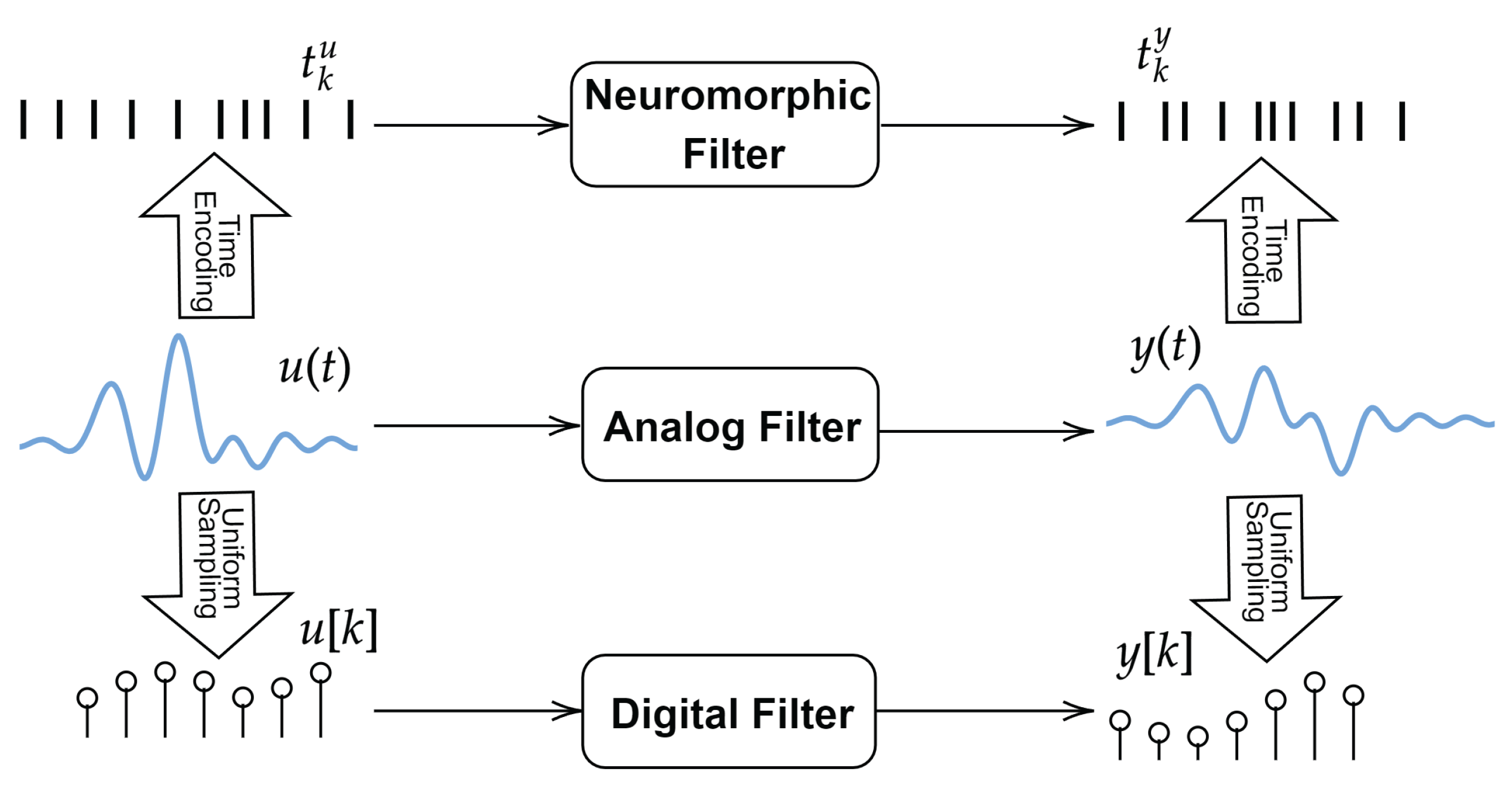
Figure 2. Output spike train prediciton for a bandlimited input. (a) Filter input and corresponding spike train. (b) Filter Output, corresponding spike train, and recovery with the indirect and proposed method.

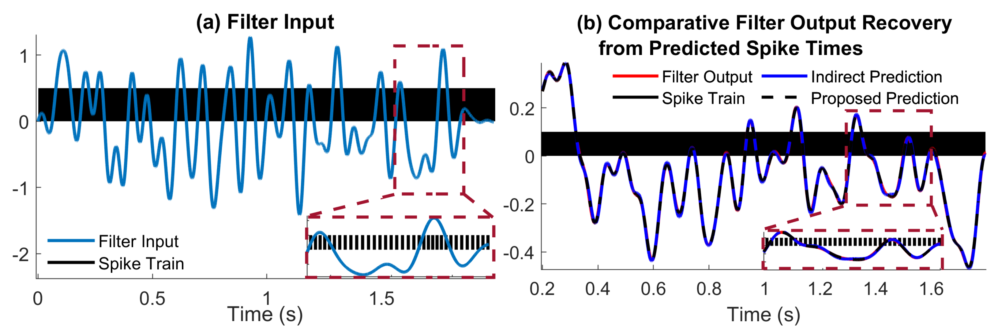
Figure 3. Spike train prediction comparative performance: the true inter-spike intervals, interposed on the predicted inter-spike intervals with the indirect and proposed methods, respectively.

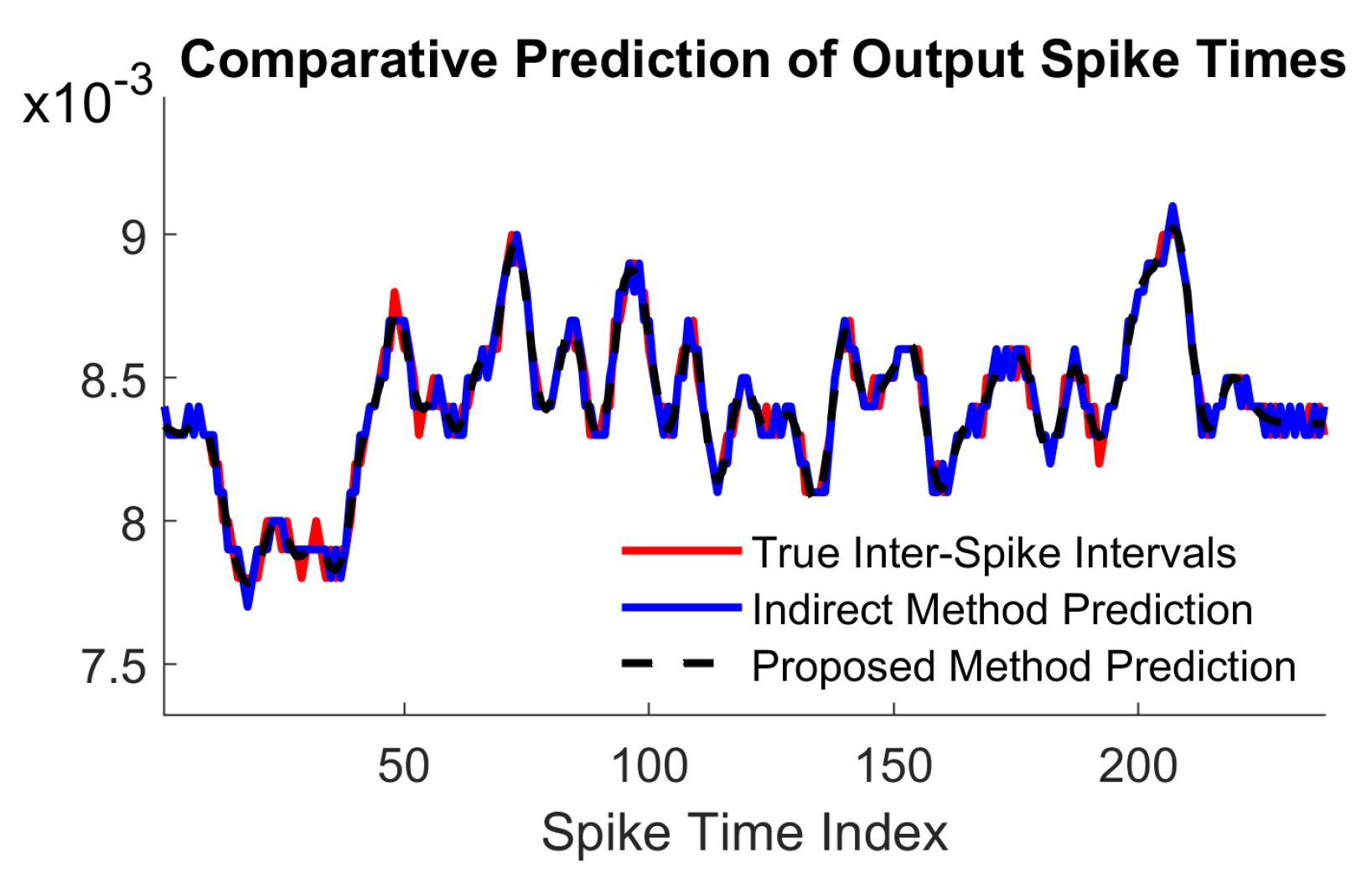
Figure 4. Output spike train prediction for uniform random noise. (a) Filter input and corresponding spike train. (b) Filter output, corresponding spike train, and recovery with the indirect and proposed method.

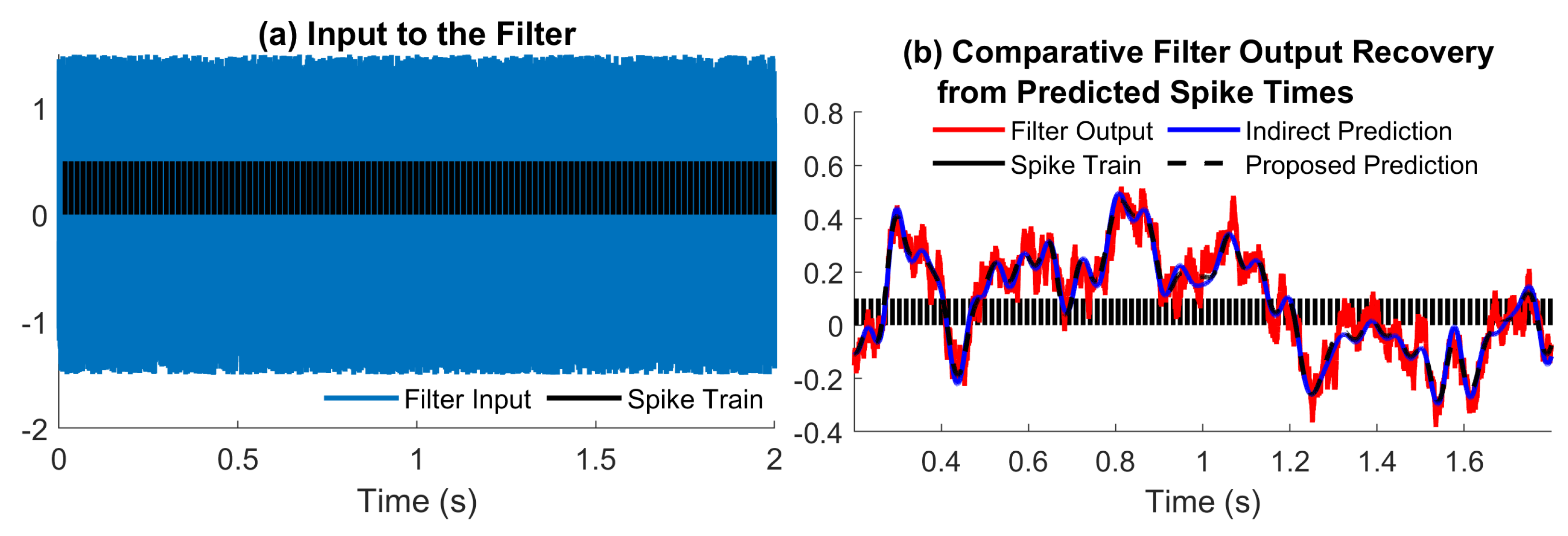
Figure 5. (a) Spike train prediction comparative performance: the true inter-spike intervals, interposed on the predicted inter-spike intervals with the indirect and proposed methods, respectively. (b) Spike train prediction comparative performance for 10 values of

δ

uniformly spaced in

[0.02, 0.1]

δ

uniformly spaced in

[0.02, 0.1]

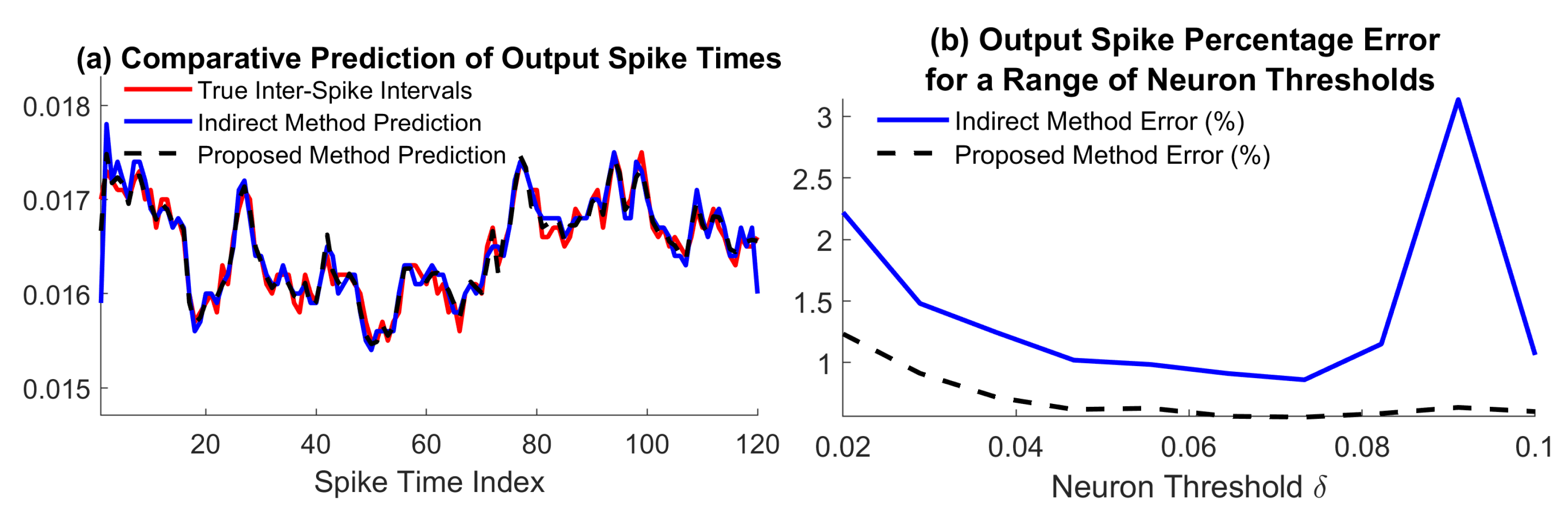
Figure 6. Filter output computation for 10 values of

δ

uniformly spaced in

[0.02, 0.1]

. (a) Analog output error. (b) Computation time.

Figure 6. Filter output computation for 10 values of

δ

uniformly spaced in

[0.02, 0.1]

. (a) Analog output error. (b) Computation time.

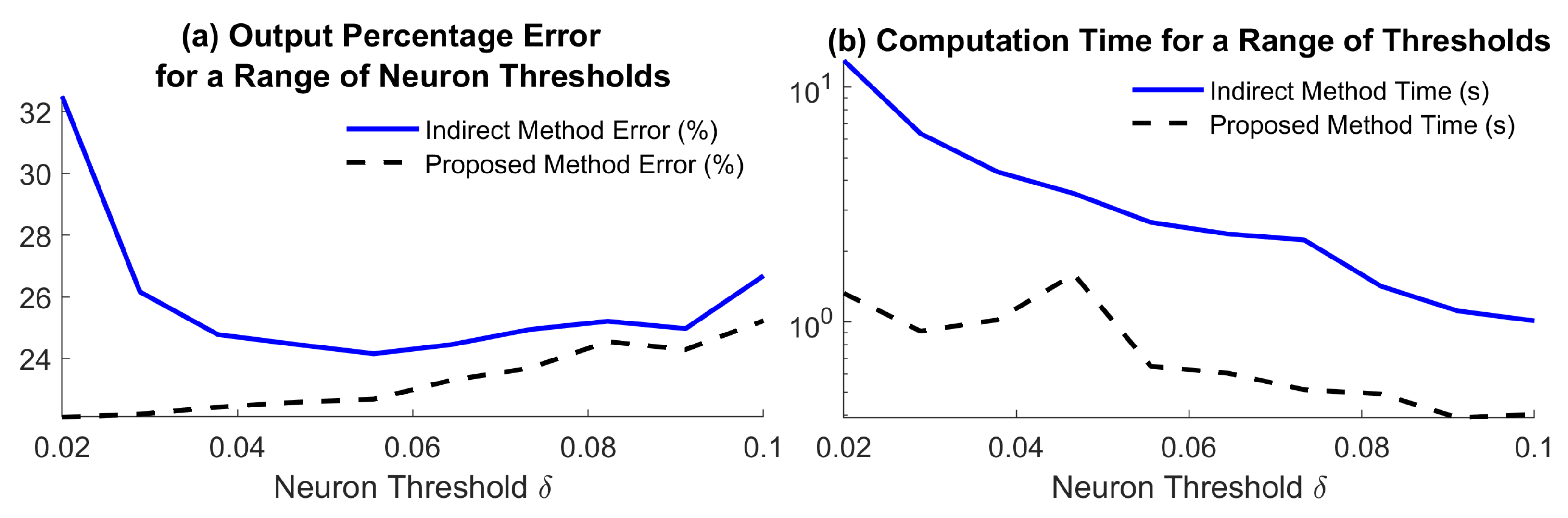
Figure 7. Bandpass filter computed via the Daubechies orthogonal wavelet 30.

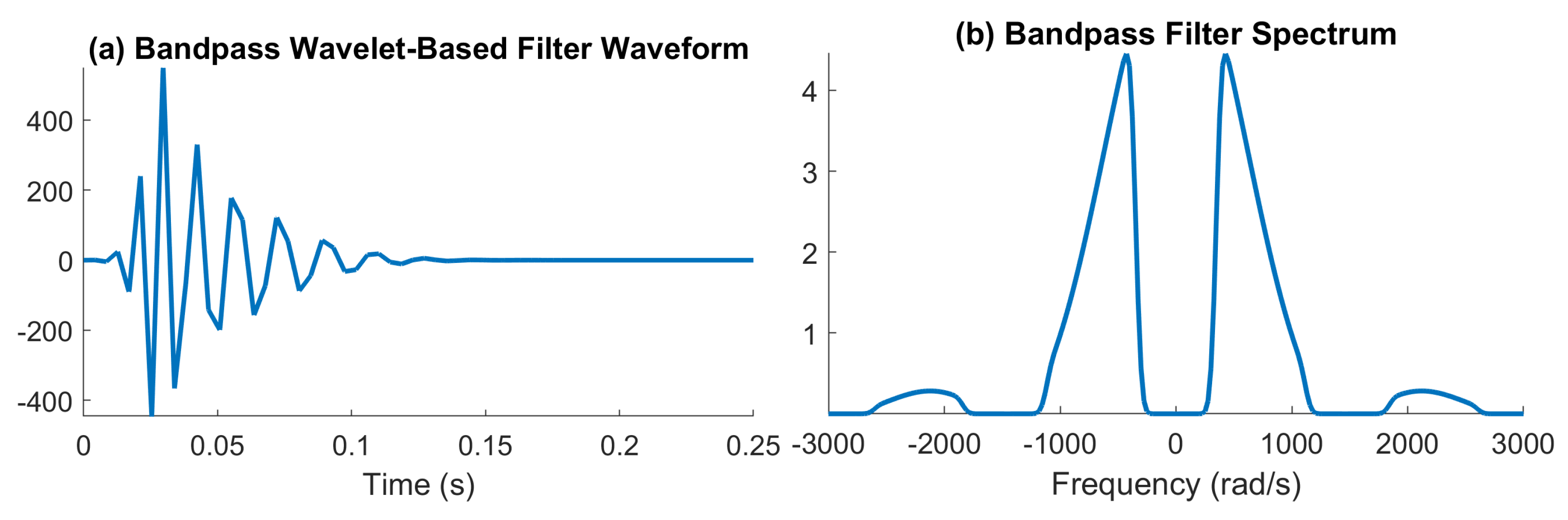
Figure 8. Filter output computation for for 11 values of the reconstruction bandwidth uniformly spaced in

[500 rad / s, 1500 rad / s]

. (a) Spike train output error. (b) Computation time.

Figure 8. Filter output computation for for 11 values of the reconstruction bandwidth uniformly spaced in

[500 rad / s, 1500 rad / s]

. (a) Spike train output error. (b) Computation time.

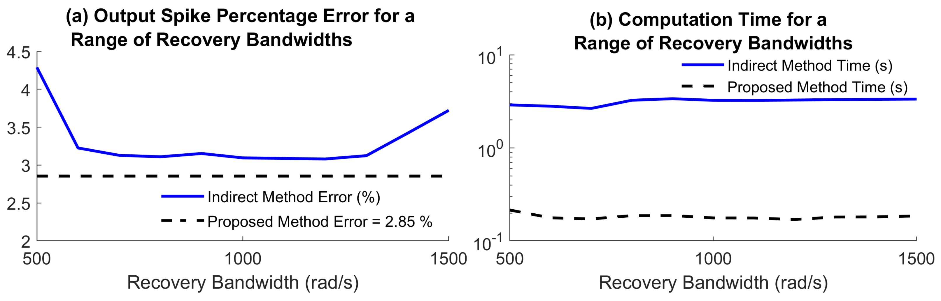
Table 1. The parameters used in our numerical simulations section are summarised below.

Example	Input	Filter	$δ$	${ERR}_{1}^{t}$ $(%)$	${ERR}_{2}^{t}$ $(%)$	${ERR}_{1}^{y}$ $(%)$	${ERR}_{2}^{y}$ $(%)$	${Time}_{1}$ (s)	${Time}_{2}$ (s)
5.1	Low pass	Low pass	$0.05$	$0.49$	$0.75$	$0.82$	$3.35$	$0.62$	$2.93$
5.2	Uniform Noise	Low pass	$0.1$	$0.6$	$1.06$	$25.2$	$26.6$	$0.32$	$0.81$
5.3	Uniform Noise	Low pass	$0 - 0.1$	$0.5 - 1.3$	$1 - 3$	$22 - 25$	$24 - 32$	$0.1 - 1$	$1 - 20$
5.4	Uniform Noise	Wavelet	$0.04$	$2.85$	$3.2$	N/A	N/A	$0.2$	3

Disclaimer/Publisher’s Note: The statements, opinions and data contained in all publications are solely those of the individual author(s) and contributor(s) and not of MDPI and/or the editor(s). MDPI and/or the editor(s) disclaim responsibility for any injury to people or property resulting from any ideas, methods, instructions or products referred to in the content.

© 2023 by the authors. Licensee MDPI, Basel, Switzerland. This article is an open access article distributed under the terms and conditions of the Creative Commons Attribution (CC BY) license (http://creativecommons.org/licenses/by/4.0/).

Copyright: This open access article is published under a Creative Commons CC BY 4.0 license, which permit the free download, distribution, and reuse, provided that the author and preprint are cited in any reuse.

MDPI Initiatives

Important Links

Choose an area of interest and we will send you notifications of new preprints at your preferred frequency.

Disclaimer

Signal Filtering Using Neuromorphic Measurements

Abstract

1. Introduction

2. Time Encoding

3. Problem Statement

4. The Proposed Neuromorphic Direct Filtering Method

5. Numerical Study

5.1. Low-Pass Filtering of a Bandlimited Signal

5.2. Low-Pass Filtering of Uniform White Noise

5.3. The Effect of Spike Density on Performance

5.4. Output Spikes Prediction for Neurons Sampling Below Nyquist Rate

6. Conclusions

Author Contributions

Funding

Institutional Review Board Statement

Data Availability Statement

Conflicts of Interest

Abbreviations

References

MDPI Initiatives

Important Links

Subscribe