1. Introduction
Titanium-niobium-alloys are excellent materials for producing superconducting magnets [
1], and are widely used in nuclear magnetic resonance spectroscopy, in magnetic resonance imaging, or in particle accelerators. Therefore, it is important to examine their physical properties. Among them, forming properties are crucial for structural applications. The mechanical behavior can be readily examined by compression testing, which does not require sample grips and larger strains can be reached before fracture, compared to tensile testing.
It is also important to describe the stress-strain behavior by analytical functions for the purpose of engineering design of the forming processes. There are several advanced formulas that are frequently used to obtain the stress as a function of plastic strain. The Johnson-Cook (‘J-C’) function includes three components that describe the effect of strain, strain rate, and temperature [
2]:
Here is the flow stress, ε is the strain, is the normalized strain rate () , T is the normalized temperature (), and A, C, n, m, , are the parameters (: melting point, ref.: reference value). The J-C approach has seven parameters, it is preferred to be used for metals whose flow curve shows a constant hardening behavior.
Similarly, Hensel and Spittel [
3] developed a model that describes the flow stress of the material in terms of strain, strain rate and temperature (‘H-S’ model), however, with the capacity of capturing not only hardening, but the softening stage as well:
Here
is initial flow stress
,
,
,
,
,
are material parameters; the H-S model contains six, originally. It is widely used, and relatively efficient; see for example: Mehtedi et al. [
4], who applied this model for hot torsional deformation of aluminum alloys.
A mathematically more efficient constitutive equation was developed by Nguyen et al. [
5], who proposed a modified Voce type constitutive equation, which is also able to capture both hardening and softening:
Here there are five parameters only (
,
,
,
,
), however, the strain rate and the temperature do not appear directly in the formula; only the strain. A first application of Eq. (3) on the Ti-6Al-4V alloy showed excellent reproduction of the experimental compression curves at high temperatures [
5]. Of course, all parameter values were depending on the temperature (the strain rate was not varied). Then, an approximation of each parameter by a second order polynom permitted to have explicit dependence on temperature, with a slight decrease in the fitting quality. In this way, the final number of coefficients was 19, and this was only for strain and temperature dependence.
Ebrahimi et al. [
6] developed a mixed-approach, using direct stress-strain formulas, together with the Zener-Hollomon relation (also called Arrhenius formula), the latter for considering the strain rate and temperature dependence. Their modeling is using two formulas; one up to the peak stress, and another after the peak stress, which includes the saturation stress as well. The number of parameters is only nine in this approach. The application is carried out on high temperature compression of Ti-IF steel, with good results. Nevertheless, it is physically difficult to justify the use of two strain hardening functions, as it implies the assumption of an instantaneous change in the microstructure processes at the peak stress.
None of the above presented modeling was used so far for studying the stress-strain behavior of Ti-Nb alloys in compression. Instead, only the Zener-Hollomon relation was employed for the construction of stress-strain curves, in the following form:
Here
Q is the activation energy,
R is the universal gas constant, and
A,
α,
n are parameters. Equation (4) contains the Zener parameter:
which allows to rewrite the Zener-Hollomon relation in the following form:
The fundamental difference of this constitutive law from the above presented ones is that it does not contain the strain as a variable, only the strain rate and the temperature; through the Z parameter. Nevertheless, it is still possible to build a stress-strain relation, because the parameters are dependent on the stress value (
), so depend on the strain as well. Such analysis was carried out by Shi-feng et al. [
7] on a TC17 (Ti-5Al-2Sn-2Zr-4Mo-4Cr) titanium alloy, and also by Sun et al. [
8] on the Ti-37 at.%Nb alloy. There is, however, a major difficulty in these works to find the parameters of the Zener-Hollomon formula. Namely, a formula for the activation energy
Q is developed by Sun et al. [
8], which is applied for a single value of the flow stress; the peak stress, therefore, its possible dependence on the stress-evolution is neglected. This is physically questionable, because it is exactly at the peak stress where there must be a change in the operating microstructure mechanisms, which necessarily should have different activation energies. Wan et al. [
9], who examined the Ti-37at.%Nb alloy in high temperature compression, reported that the relationship between
Z and
and
1/T does not satisfy a linear relationship when the deformation temperature is in the range of 790 - 940 °C for strain rates between 0.001 s
-1 and 10 s
-1, therefore, the Arrhenius equation is questionable.
Wan et al. [
9] also applied a new computation technique, called ‘GA-LSSVM’ algorithm, which was initially developed in agriculture industry [
10]. This technique is using non-linear mapping with artificial intelligence, without constitutive law, by dividing the measured data sets into ‘known’ and ‘unknown’ categories and predicting in this way the whole data set. While it was successfully used for the compression of the Ti-37at.%Nb alloy at high temperatures, its use in metallurgical engineering is complex, while not leading to better results than using a constitutive law (mean relative error was 2.74%).
There are limited studies on the plastic behavior of Ti-Nb alloys at high temperatures, while there are comprehensive works on pure Ti [
11] and pure Nb [
12]. High Nb content is required for superconductivity and magnetic applications. Only Sun et al. [
8] and Wan et al. [
9] examined such alloy; in both studies the Ti-37 at.%Nb alloy was investigated.
The above short analysis of the state of art in stress-strain curve modeling of high temperature compression of metals shows that it is more promising to employ constitutive equations that contain strain as direct variable, compared to the Arrhenius type indirect approach.
Strain hardening/softening can be also produced by the evolution of the crystallographic texture of the material during plastic deformation. Hard texture components increase the yield stress while weaker ones are reducing it. This effect can be examined by suitable polycrystal modeling, like the viscoplastic self-consistent (VPSC) model [
13]. For example, it was observed in torsion of Mg that the initial strain hardening stage was due to the evolution of the texture, which could be modeled by the VPSC approach, without introducing any intrinsic hardening into the simulation [
14].
In the present study, the Voce type modified constitutive equation proposed by Nguyen et al. [
5] was used for describing the hot compression stress-strain curves of Ti57-Nb43 at high temperatures, from 700 to 1000 °C, at four strain rates. It is shown that instead of five, only four parameters are enough for a good reproduction of the experimental data. With the help of new polynomial functions, the parameters were explicitly expressed as a function of the temperature and strain rate. Good agreements have been reached between the modeled and experimental data in the range of 800 – 1000 °C and 0.01 to 1 s
-1 testing, with only 1.48% general average relative error.
It is also shown in the present work that the strain hardening behaviour is not influenced by the texture evolution in the present Ti-Nb alloy. The observed softening in the experiment is the result of dynamic recrystallization, which could be confirmed by detailed examination of the microstructure. It is important to identify the mechanisms that control the strength of the material. This is the first study where the relation between strength and texture evolution is examined in compression or rolling of Ti-Nb alloys.
6. Texture measurements and VPSC modeling results
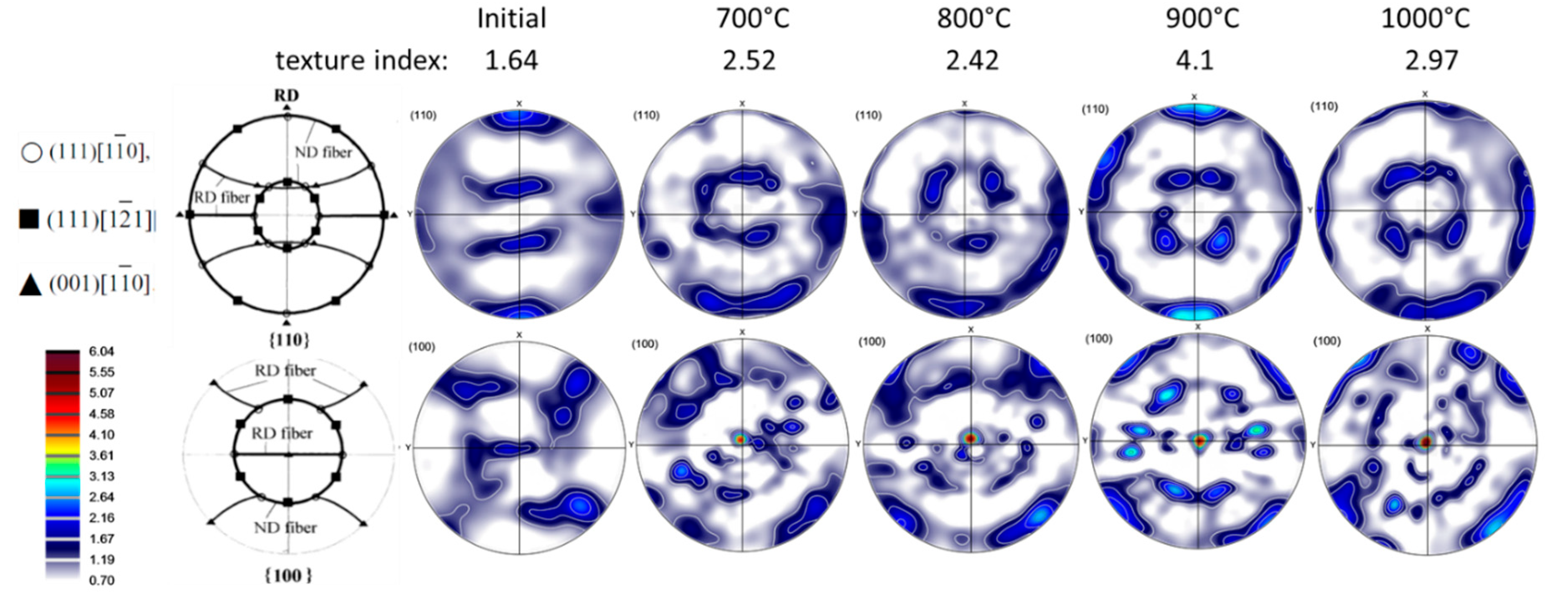
The raw pole figure measurements were processed to obtain the recalculated ones from the ODF with the help of the ATEX software [
19]. The measured crystallographic textures of the initial material, and that of the samples deformed at 700, 800, 900 and 1000 °C at the compression strain rate of 0.1 s
-1 are presented in (110) and (100) pole figures in
Figure 10. The phase is b.c.c., for all temperatures in this alloy. The initial state of the material was a hot-rolled plate, from which cylindrical shaped samples were cut out in the normal direction of the plate. Therefore, the initial state of the material was a rolling texture (
Figure 10). Because a texture was already existing in the material before testing, the original RD, TD, and ND directions were tracked on the samples for all texture measurements, and the textures are presented in that reference system. The ideal orientations of b.c.c. rolling textures are also presented in the (110) and (100) pole figures in
Figure 10 (from Ref. [
20]). As can be seen from the pole figures, the initial texture contained the two major ideal fibers of rolling; called RD and ND fibers, which are defined by <110> parallel to RD and <111> parallel to ND, respectively. Nevertheless, these fibers did not present uniform intensities; three ideal orientations were preferred: the
, the
, and the
, identified in the key pole figures. After deformation, the texture changed slightly: the ND fiber became more uniform, while along the RD fiber, the
component became the major texture component. This component is an ND-45° rotated cube position. There are also noticeable variations in the strength of the textures as a function of processing temperature; the texture index is indicated in
Figure 10. The initial texture is actually quite weak with its index of 1.64 (for a random texture it is 1.0). There is some strengthening due to the deformation at 700 and 800 °C up to about a value of 2.5. The texture is the strongest at 900 °C, where it displays an index of 4.1. At 1000 °C its intensity is 2.97. One can see in
Figure 10 that the textures are slightly rotated around the TD axis at 700, 800 and 1000 °C which can be due to some misalignment in the sample positions; the texture seems the most symmetric at 900 °C. Note that the textures were processed without applying sample symmetries. Such operation would reduce the texture intensity and can only be applied if the initial texture was symmetric, and the deformation was as well, moreover, if the grain size was sufficiently small for good statistics. While the initial texture was relatively symmetric and the compression as well, the grain sizes were not small enough at high temperatures due to recrystallization (about 200 µm), so some spotty nature of the measured textures can be seen in the pole figures.
The VPSC polycrystal simulations were carried out using the finite-element-calibrated version of the Metz-VPSC code, see Ref. [
13] for the modeling approach. The value of the so-called interaction parameter (α in the localization equation of the VPSC model) was chosen very low (0.01), meaning that the stress states in the grains of the polycrystal were nearly equal to the macroscopic one (‘static’ approach). As the material was in b.c.c. state, the 12
and 12
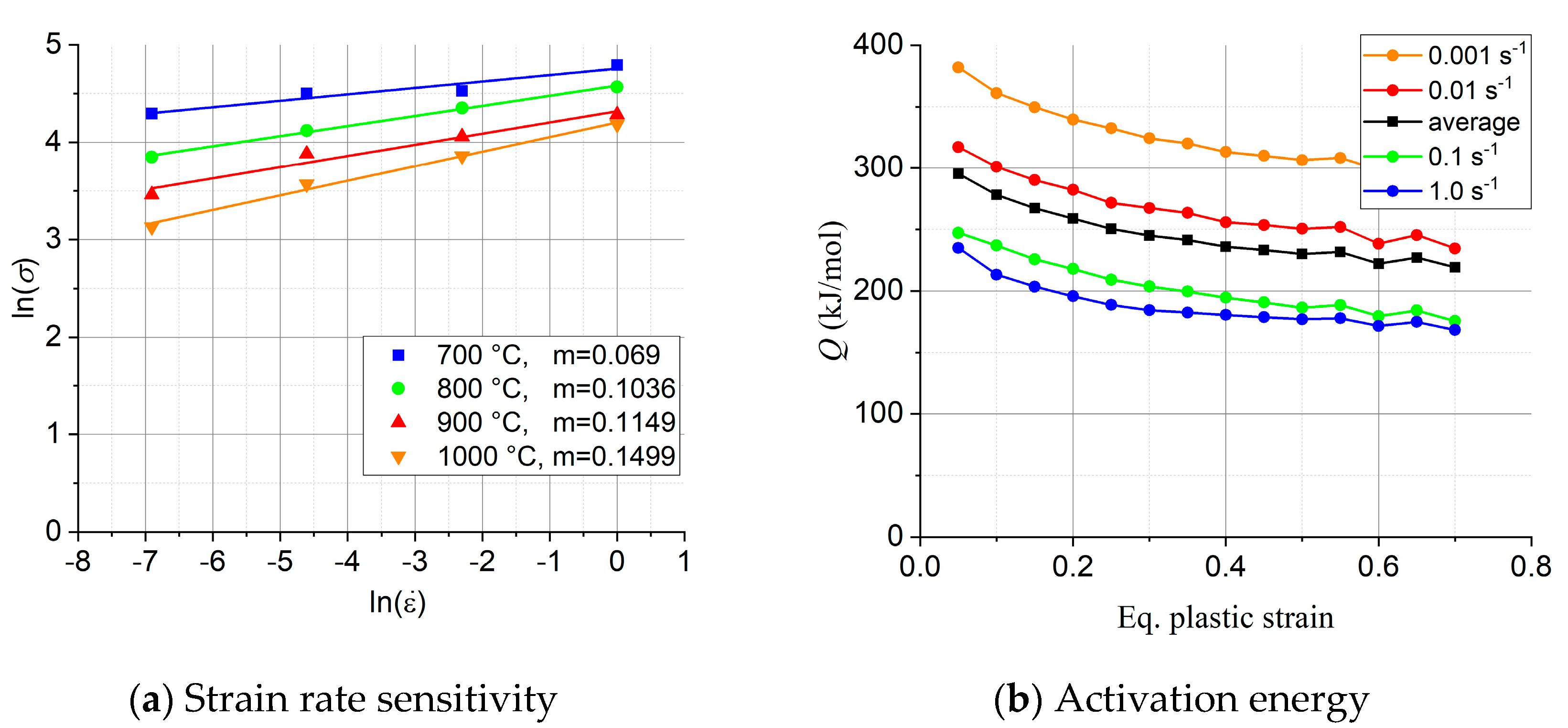
slip systems were used as possible slip systems with equal strengths. The strengths of the slip system were kept constant during the simulation, i.e., strain hardening was not simulated. This was done in order to examine only the effect of the evolution of the texture on the compression stress-strain curve. The value of 0.1 was used for the viscoplasticity index of slip (the ‘m’ parameter), which is the average value of the measured strain rate sensitivities at high temperatures of this alloy (see
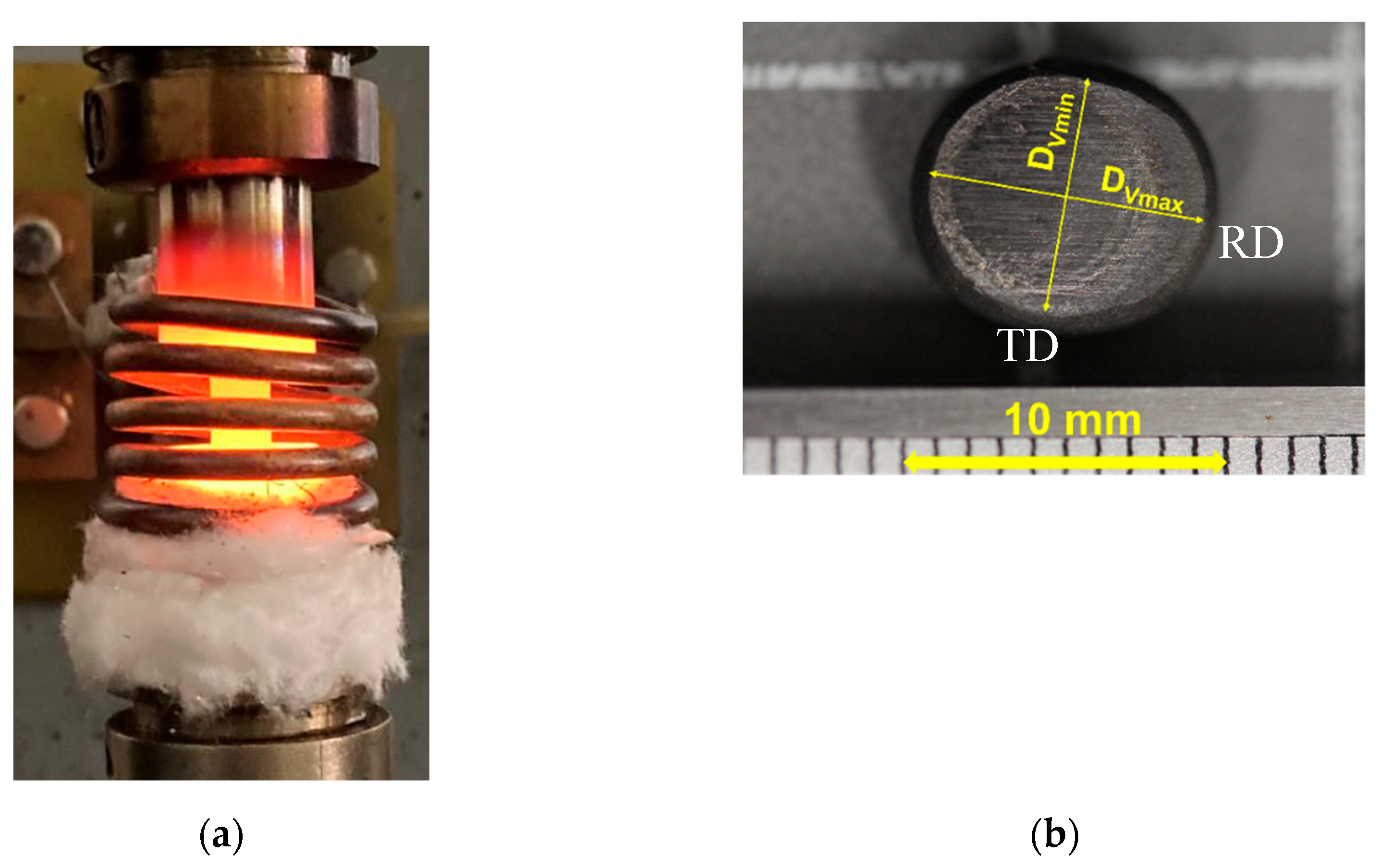
Figure 5a). The initial texture was discretized by the ATEX software to 5000 grain orientations and used for the compression simulation. The macroscopic imposed strain rate tensor was imposed without shear components, and the relative values of the three normal strain components were set according to the experimental observation. Namely, as mentioned above in the experimental part, the cross-section of the cylindrical samples became elliptic (see
Figure 1b), so that the strain ratio between the RD and TD strains was about 2.0. This situation was imposed in the simulation. The VPSC calculation was carried out in 50 small strain increments with an increment size of 0.01 to obtain the final true compression strain of -0.5.
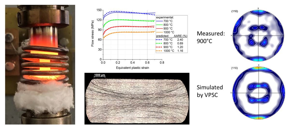
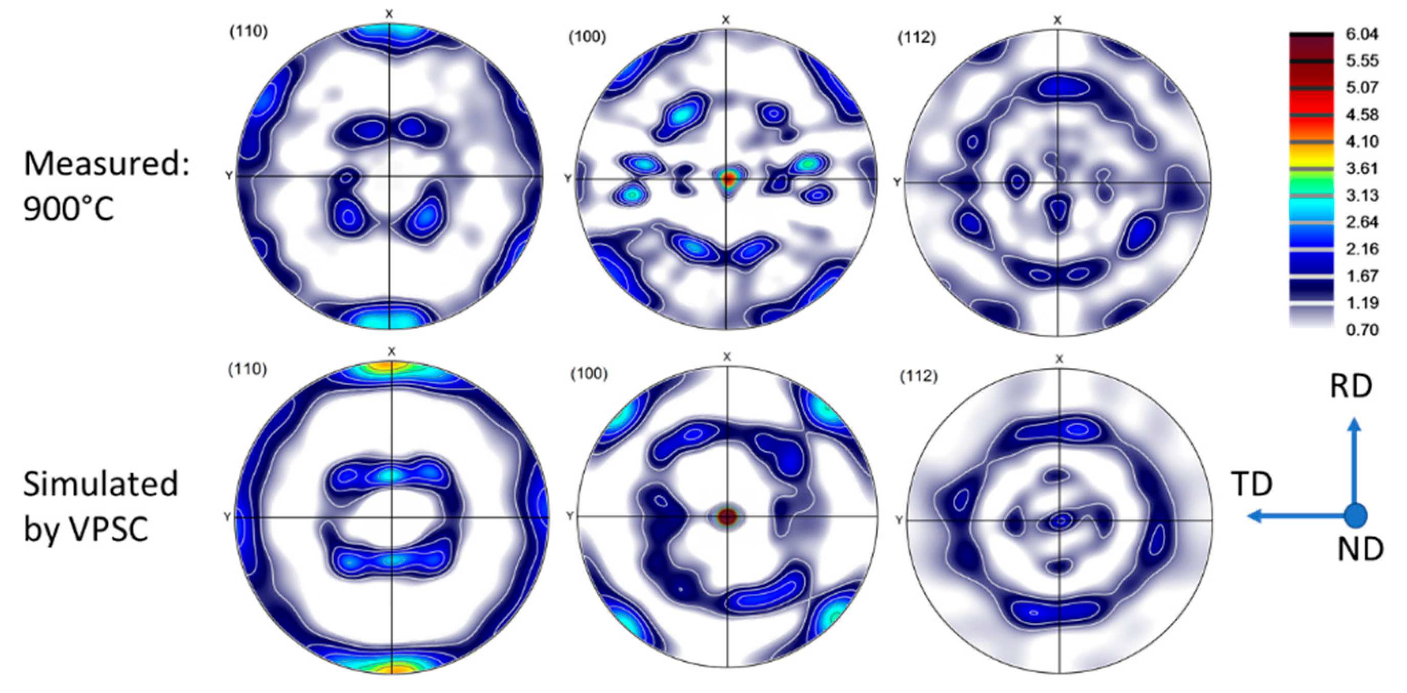
The simulated textures are displayed in
Figure 11 in three pole figures ((110), (100), and (112)), in comparison with the experimental texture measured at 900 °C. As the textures were similar at all temperatures, only one simulation was carried out. There is a good agreement between the simulation and experiment, even some of the details are reproduced by the simulation. Concerning the evolution of the compression stress as a function of strain, only a slight increase was predicted by the VPSC model; up to 1.5% in flow stress.
7. Discussion
As was pointed out in the Introduction, the analytical description of the stress-strain response of the investigated alloy is important for the forming processes that are needed for its use in applications. This alloy was plastically deformed at high temperatures where dynamic recrystallization can take place. Therefore, its stress-strain behavior is complex, includes strain hardening as well as softening stages. The mathematical description of such curves requires several parameters, that are varying when the temperature and the strain rate are changed. It is important to describe the curves with minimum number of coefficients. The modified Voce equation (Eq. 13), presented by Nguyen et al. [
5], is a very suitable function for this purpose, and its applicability for the experiments carried out in this work has been demonstrated. One of the most important results of the present work is that the number of parameters of the modified Voce equation can be reduced from five to four for the case of compression of the Ti-Nb alloy. The other major result is the approximation of the four coefficients by a suitable polynom, with two variables, that are the temperature and the strain rate. One advantage of such procedure is a further reduction of the number of coefficients. Indeed, for the present experiments, where four temperatures and four strain rates were considered, the total number of coefficients were 4 x 4 x 4 = 64. For the polynomial description it was only 4 x 8 = 32. The other advantage is that the polynom can be used at any temperature and strain rate, while the non-polynomial approach is only valid for the 4 x 4 measured cases, so does not have a predictive capacity.
Nevertheless, it is also true that the polynomial approach was not applicable to the whole investigated temperature and strain rate ranges. It has been found that it was not working well for the lowest temperature (700 °C), and for the lowest strain rate (0.001 s
-1). From industrial point of view, the very low strain rate is not an issue because industrial plastic forming processes are done at high strain rates. We have actually examined material behavior up to 1.0 s
-1, which is in the range of industrial applications. Concerning the deviation at 700 °C, it can be explained by the strain localization in form of an X, well visible on the metallographic image in
Figure 3a. Such localization is due to the unstable nature of the deformation at that temperature, which is to be avoided, so the forming operation should be done at higher temperatures. At the same time, the strain rate sensitivity parameter m was found relatively low and out of trend at 700 °C, which could have also contributed to the localization of the deformation. It is well known that higher strain rate sensitivity delays strain localization, so forming at high temperatures, where strain rate sensitivity is high, is advantageous for formability. Note that Sarkar et al. [
21] also observed strain localization below 1000 °C in the Nb–1Zr–0.1C alloy, that led to two distinctly different domains under the conditions of hot deformation.
The texture measurements together with the VPSC modeling were helpful for clarifying the role of the texture in the behavior of the material during compression. Two effects were examined: the shape change and the strain hardening. Due to the previous hot rolling of the samples, there was a rolling texture in the material before compression. Therefore, the strain response was not the same in the RD and TD directions, leading to twice more strain in the RD direction than in TD. This effect led to an elliptical shape of the cross-section of the sample, so the texture played an important role in the deformation. For obtaining information on the role of the texture in the strain hardening behavior of the alloy, it was only possible by doing polycrystal plasticity simulations for which purpose the VPSC model was used. VPSC modeling provides two important results: the material strength and the evolution of the crystallographic texture. Once the simulation is reproducing well the experimental texture, the effect on the strain hardening is also correctly obtained. It was found in the present compression experiments that there was no significant effect of the evolution of the texture on the flow stress of the material; only about 1.5% increase was observed during the compression strain of 0.5. This can be understood by examining the texture changes during deformation which were found to be relatively small. Indeed, the strain mode did not change dramatically when compression was applied after rolling. The strain rate tensors (
D) for compression and for rolling were the following:
where
is the compression strain rate. The relatively small difference led to a small evolution of the texture, so the strength was not influenced significantly, it could be still characterized by the texture components of rolling. Nevertheless, it is important to point out that the initial texture was determinant in the simulation of the texture. Namely, for isotropic texture, the compression strain mode becomes axisymmetric, and the texture evolves into a typical axisymmetric texture which can be characterized by two ideal fibers: <001> || ND and <111> || ND, see such simulation result in
Figure 12. A comparison of this predicted texture with the simulated and experimental ones displayed in
Figure 11 shows clearly that it is important to consider the anisotropy of the material before compression for achieving good modeling of the texture evolution.
Figure 1.
(a): Heating of the specimen up to the forming temperature. (b): Top view of the compressed material.
Figure 1.
(a): Heating of the specimen up to the forming temperature. (b): Top view of the compressed material.
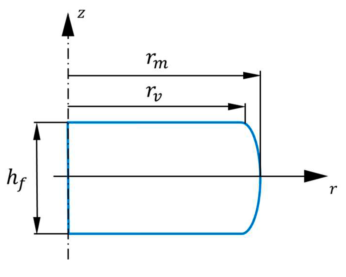
Figure 2.
Geometrical parameters of the specimen after compression.
Figure 2.
Geometrical parameters of the specimen after compression.
Figure 3.
Micrographs of two specimens deformed at 700°C (a) and 1000°C (b) with strain rate of 0.01 s-1 to a height reduction of 50%.
Figure 3.
Micrographs of two specimens deformed at 700°C (a) and 1000°C (b) with strain rate of 0.01 s-1 to a height reduction of 50%.
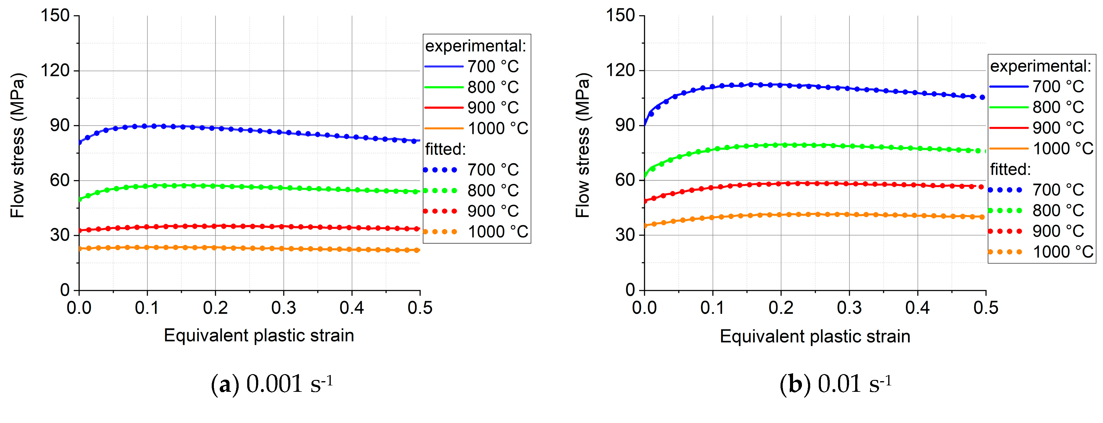
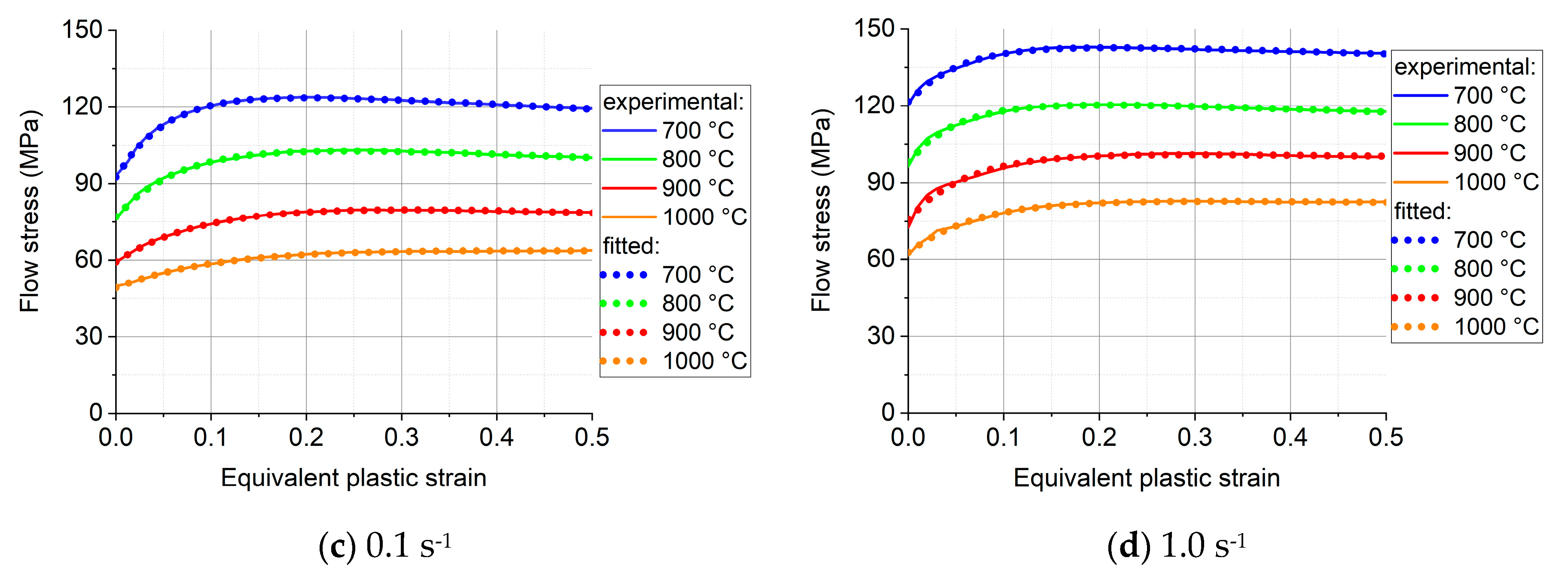
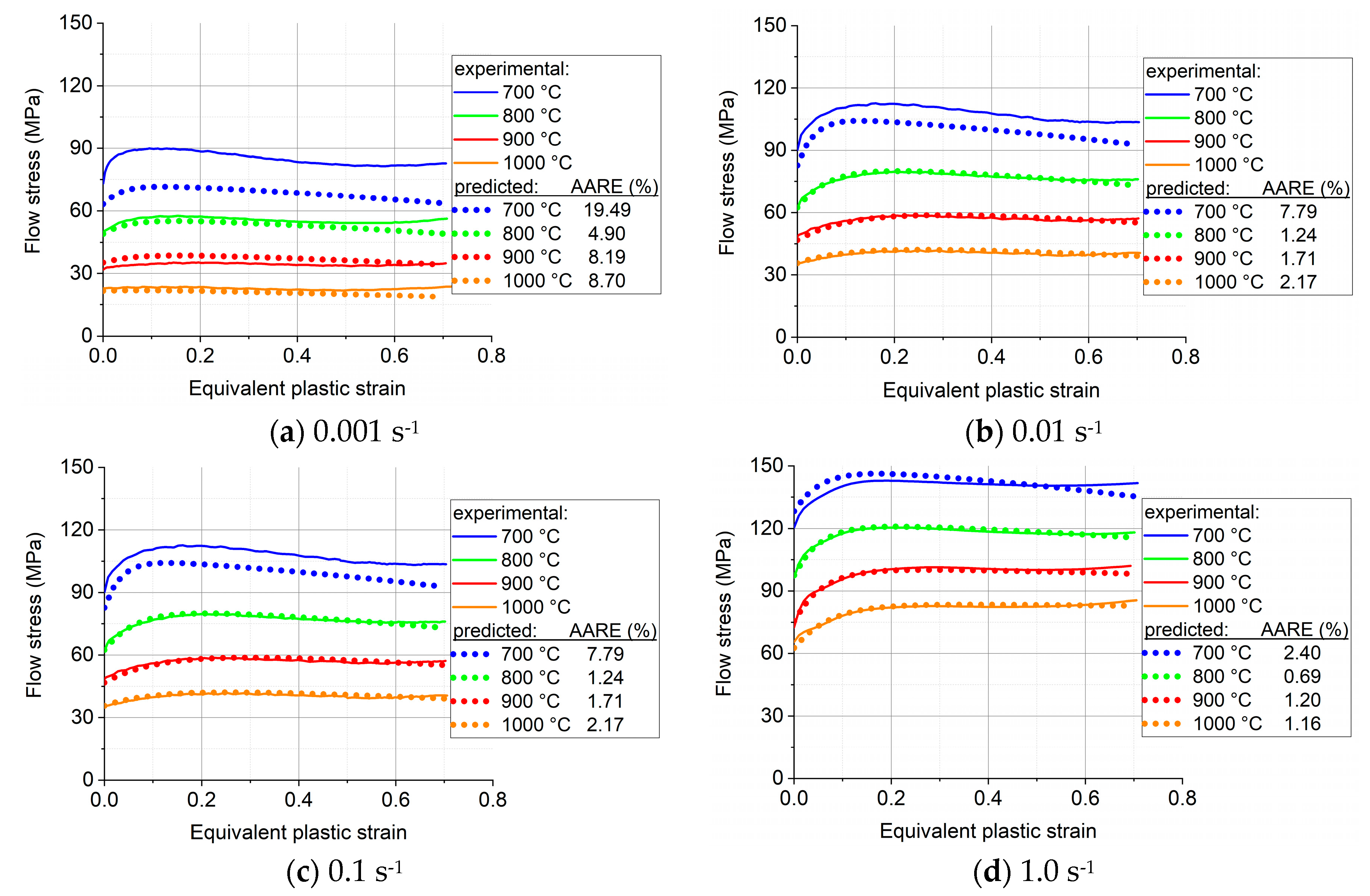
Figure 4.
Measured and fitted flow stress-strain curves of Ti57-Nb43: (a) 0.001 s-1, (b) 0.01 s-1, (c) 0.1 s-1, (d) 1.0 s-1. The fitted curves were derived from Eq. (13).
Figure 4.
Measured and fitted flow stress-strain curves of Ti57-Nb43: (a) 0.001 s-1, (b) 0.01 s-1, (c) 0.1 s-1, (d) 1.0 s-1. The fitted curves were derived from Eq. (13).
Figure 5.
(a): Strain rate sensitivity diagram at zero plastic strain, (b): Variation of activation energy as a function of the equivalent plastic strain and strain rate.
Figure 5.
(a): Strain rate sensitivity diagram at zero plastic strain, (b): Variation of activation energy as a function of the equivalent plastic strain and strain rate.
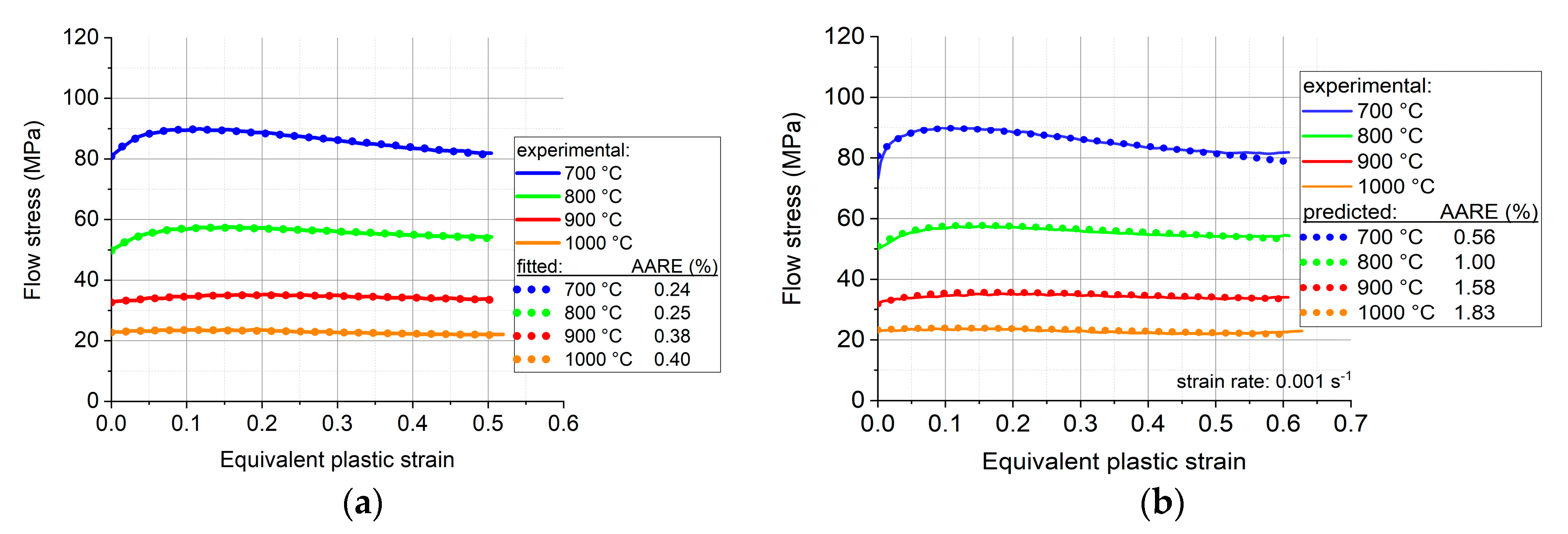
Figure 6.
The measured and their fitted curves obtained by using Eq. (13) for the compression strain rate of 0.001 s-1, at four temperatures. (a): separate fit for each curve, (b): fit by using polynomial coefficients for the four parameters, expressed directly as a function of temperature.
Figure 6.
The measured and their fitted curves obtained by using Eq. (13) for the compression strain rate of 0.001 s-1, at four temperatures. (a): separate fit for each curve, (b): fit by using polynomial coefficients for the four parameters, expressed directly as a function of temperature.
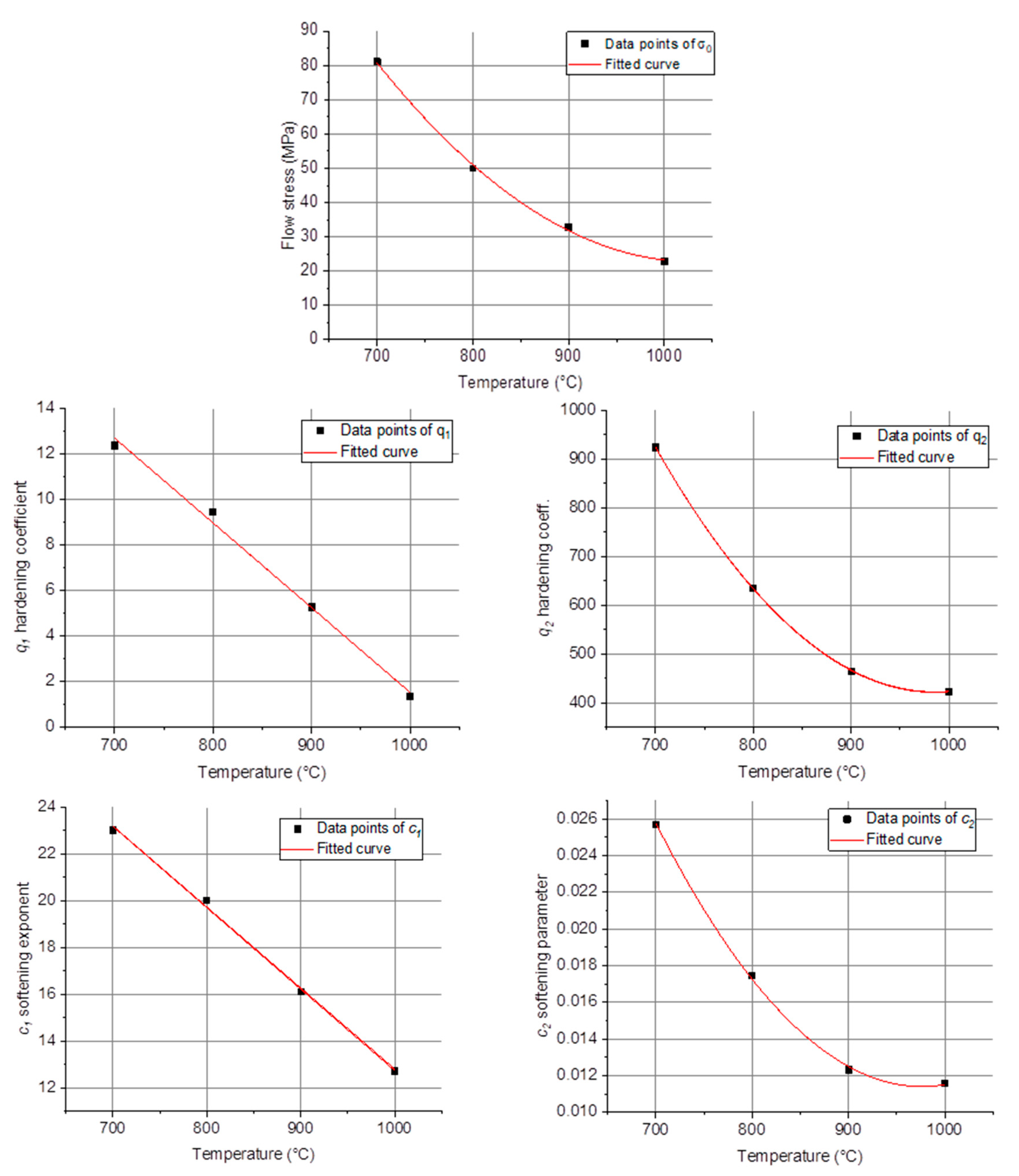
Figure 7.
Dependence of the yield stress, and the , , ,
Figure 7.
Dependence of the yield stress, and the , , ,
Figure 8.
Measured and polynomial-predicted stress-strain curves using the function defined in Eq. (15) for the four strain rates and four temperatures.
Figure 8.
Measured and polynomial-predicted stress-strain curves using the function defined in Eq. (15) for the four strain rates and four temperatures.
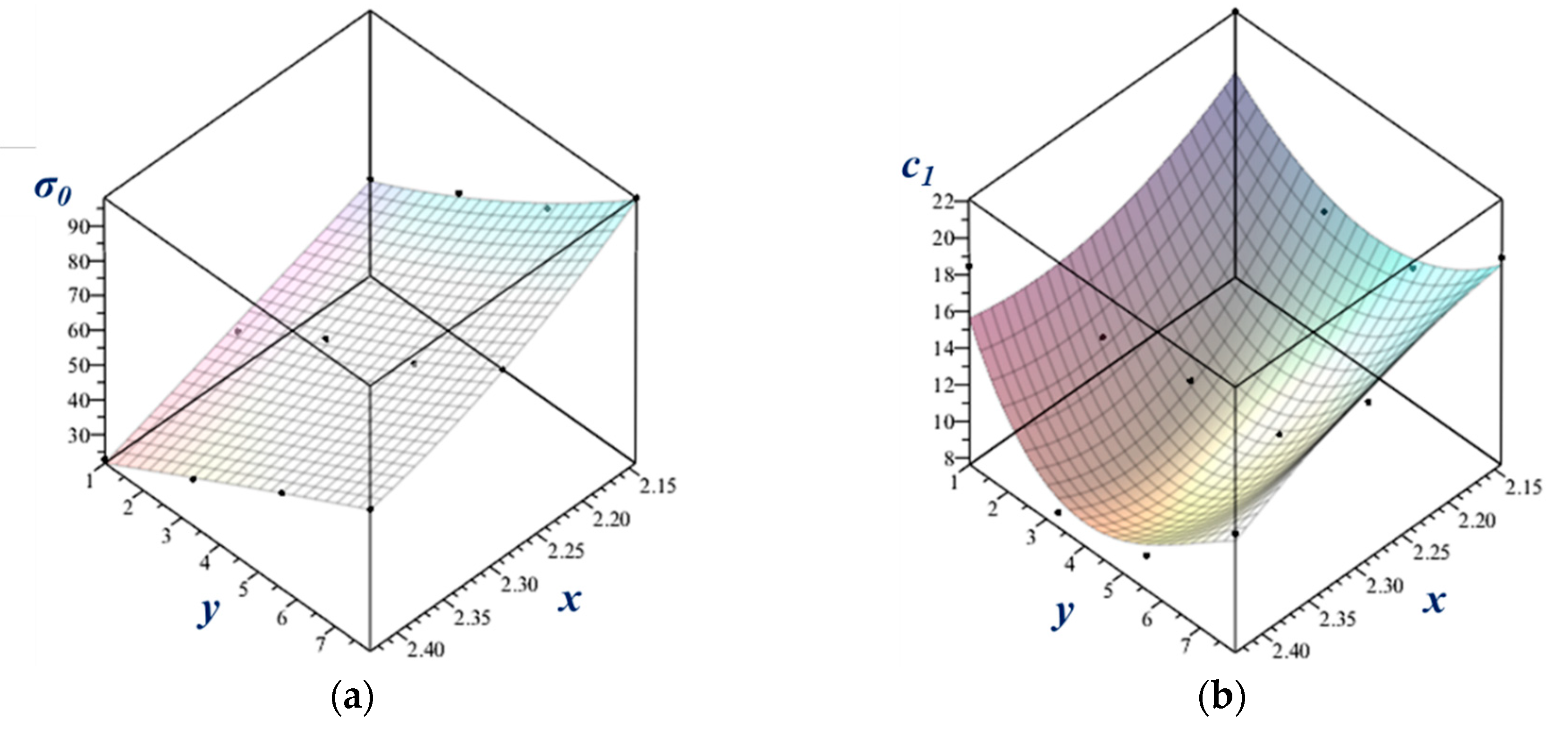
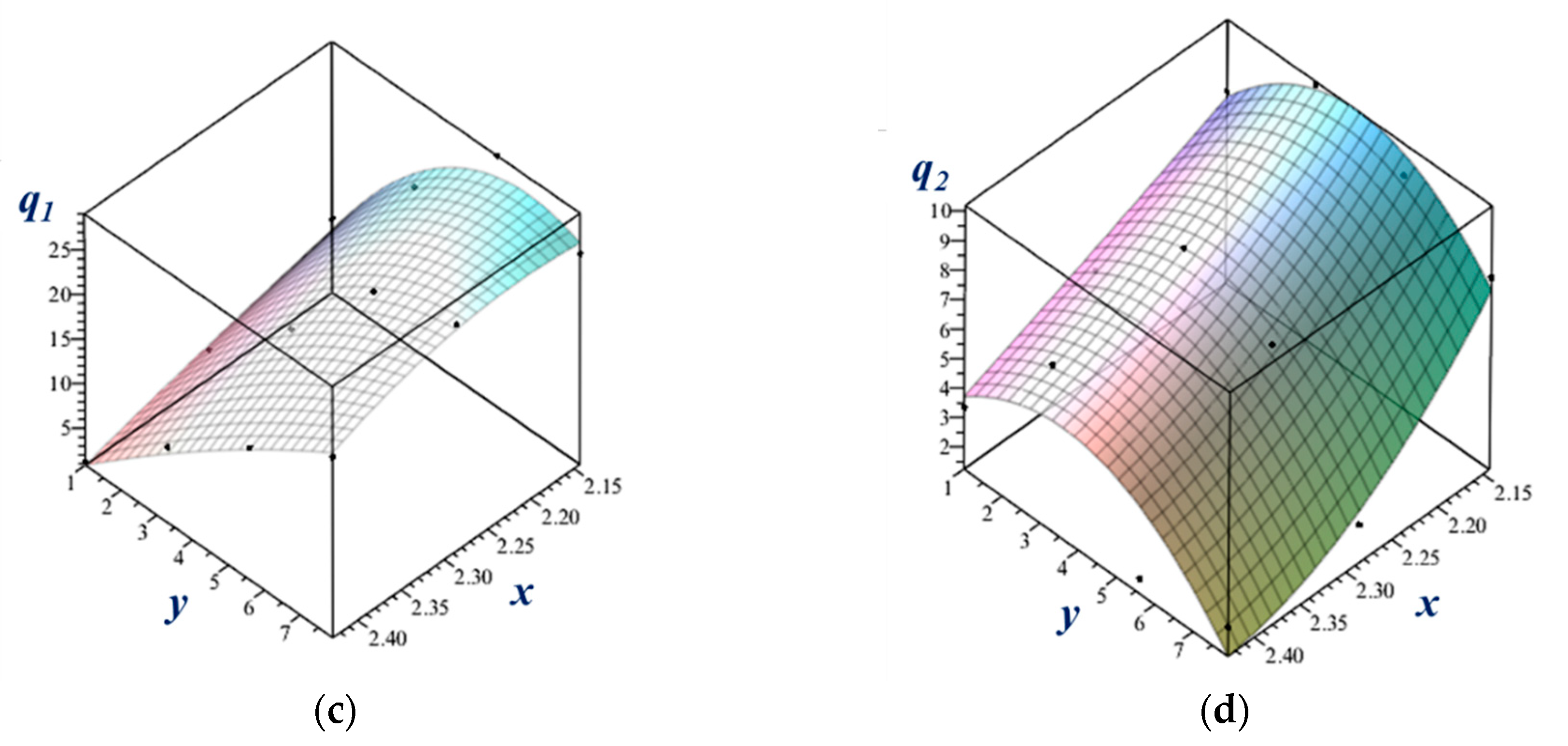
Figure 9.
Fitted surfaces on the data points of the material parameters as a function of the strain-rate and temperature.
Figure 9.
Fitted surfaces on the data points of the material parameters as a function of the strain-rate and temperature.
Figure 10.
Measured textures shown in (110) and (100) pole figures. The ideal fibers of b.c.c. rolling textures are also shown with the identification of three major ideal orientations.
Figure 10.
Measured textures shown in (110) and (100) pole figures. The ideal fibers of b.c.c. rolling textures are also shown with the identification of three major ideal orientations.
Figure 11.
Measured and simulated textures in hot compression of Ti-Nb in three pole figures ((110), (100), and (112)).
Figure 11.
Measured and simulated textures in hot compression of Ti-Nb in three pole figures ((110), (100), and (112)).
Figure 12.
Simulated texture for an axisymmetric compression of -0.5 using random initial texture represented by 5000 grain orientations, displayed in (111), (100), and (110) pole figures.
Figure 12.
Simulated texture for an axisymmetric compression of -0.5 using random initial texture represented by 5000 grain orientations, displayed in (111), (100), and (110) pole figures.
Table 1.
The chemical composition of the Ti57-Nb43 alloy (weight %).
Table 1.
The chemical composition of the Ti57-Nb43 alloy (weight %).
| Ti |
Nb |
Au |
Fe |
Pd |
Mn |
rest |
| 56.54 |
42.81 |
0.18 |
0.12 |
0.12 |
0.06 |
0.16 |
Table 2.
The parameter values of Eq. (13) for the measurements carried out at 0.001 s-1.
Table 2.
The parameter values of Eq. (13) for the measurements carried out at 0.001 s-1.
Parameter
values |
Temperature (°C) |
| 700 |
800 |
900 |
1000 |
|
[MPa] |
80.84 |
49.76 |
32.62 |
22.75 |
|
[MPa] |
12.36 |
9.433 |
5.268 |
1.343 |
|
[MPa] |
924.0 |
634.2 |
464.7 |
422.9 |
|
23.01 |
20.01 |
16.10 |
12.71 |
|
0.0257 |
0.01743 |
0.01231 |
0.01156 |
Table 3.
The polynomial coefficients for fitting the parameters of Eq. (13) as a function of temperature for the measurements carried out at 0.001 s-1.
Table 3.
The polynomial coefficients for fitting the parameters of Eq. (13) as a function of temperature for the measurements carried out at 0.001 s-1.
| Parameters |
Polynomial coefficients |
| constant |
Linear coefficient |
Second order coefficient |
|
|
[MPa] |
584.9068 |
-1.0905 |
5.2884ꞏ10-4
|
|
|
[MPa] |
38.7562 |
-0.0372 |
0 |
|
|
[MPa] |
6436.6547 |
-12.216 |
0.0062 |
|
|
47.4508 |
-0.0346 |
0 |
|
|
0.1906 |
-3.6709ꞏ10-4
|
1.8798ꞏ10-7
|
|
Table 4.
Fitted values of the parameters in Eq. (15) at four temperatures and four strain rates.
Table 4.
Fitted values of the parameters in Eq. (15) at four temperatures and four strain rates.
| Strain rate |
Temperature |
σ0 |
q1 |
c1 |
q2 |
AARE |
| [s-1] |
[°C] |
[MPa] |
[MPa] |
|
[MPa] |
[%] |
| 0.001 |
700 |
80.773 |
11.531 |
26.211 |
17.109 |
1.52 |
| 800 |
49.745 |
9.107 |
22.132 |
7.776 |
0.27 |
| 900 |
32.638 |
4.064 |
9.465 |
4.837 |
0.39 |
| 1000 |
22.771 |
1.257 |
18.480 |
3.334 |
0.52 |
| 0.01 |
700 |
92.430 |
23.544 |
20.833 |
16.459 |
0.35 |
| 800 |
63.451 |
19.091 |
14.618 |
10.097 |
0.34 |
| 900 |
48.654 |
12.790 |
10.499 |
7.699 |
0.33 |
| 1000 |
35.192 |
9.343 |
8.430 |
6.898 |
0.38 |
| 0.1 |
700 |
92.478 |
34.473 |
19.044 |
12.130 |
0.15 |
| 800 |
76.974 |
29.011 |
14.955 |
9.131 |
0.25 |
| 900 |
59.322 |
23.527 |
10.981 |
6.547 |
0.18 |
| 1000 |
49.209 |
15.676 |
9.524 |
1.759 |
0.21 |
| 1.0 |
700 |
121.570 |
23.264 |
18.349 |
7.097 |
0.21 |
| 800 |
98.099 |
24.455 |
18.944 |
7.757 |
0.28 |
| 900 |
75.721 |
26.230 |
16.174 |
2.538 |
0.59 |
| 1000 |
62.656 |
21.128 |
14.144 |
2.232 |
0.31 |
Table 5.
Estimated coefficients of the polynomials.
Table 5.
Estimated coefficients of the polynomials.
| Params. |
σ0 (x,y) |
q1 (x,y) |
c1 (x,y) |
q2 (x,y) |
| a2 |
-3.27538 |
0.0 |
-13.46825 |
0.0 |
| a3 |
13.95439 |
2.011577 |
62.19368 |
0.10279 |
| a4 |
59.76368 |
-12.28321 |
102.38188 |
8.67384 |
| a5 |
-14.60045 |
-4.96277 |
-71.1329 |
-0.44966 |
| a6 |
-49.61801 |
-4.02339 |
-6.81293 |
-5.871106 |
| a7 |
-267.96893 |
39.68338 |
-474.14841 |
-41.70084 |
| a8 |
304.47517 |
-20.23071 |
543.23392 |
51.54085 |
| a9 |
126.90537 |
8.62717 |
24.51490 |
15.28197 |
