Submitted:
22 October 2023
Posted:
23 October 2023
You are already at the latest version
Abstract
Keywords:
1. Introduction
2. Material and Method
2.1. Data collection and processing
2.2. Sample preparation
2.3. Data Splitting
2.4. Data Scaling and feature extraction
2.5. Machine Learning Algorithm
2.5.1. XGBoost
2.5.2. Random Forest
2.5.3. Neural network models(MLP Regressor)
2.6. GridsearchCV
2.7. Evaluation Criteria
2.8. Optimal pipeline
2.9. Generalization Ability Verification
2.10. Result Demonstration
3. Data Preparation and Description
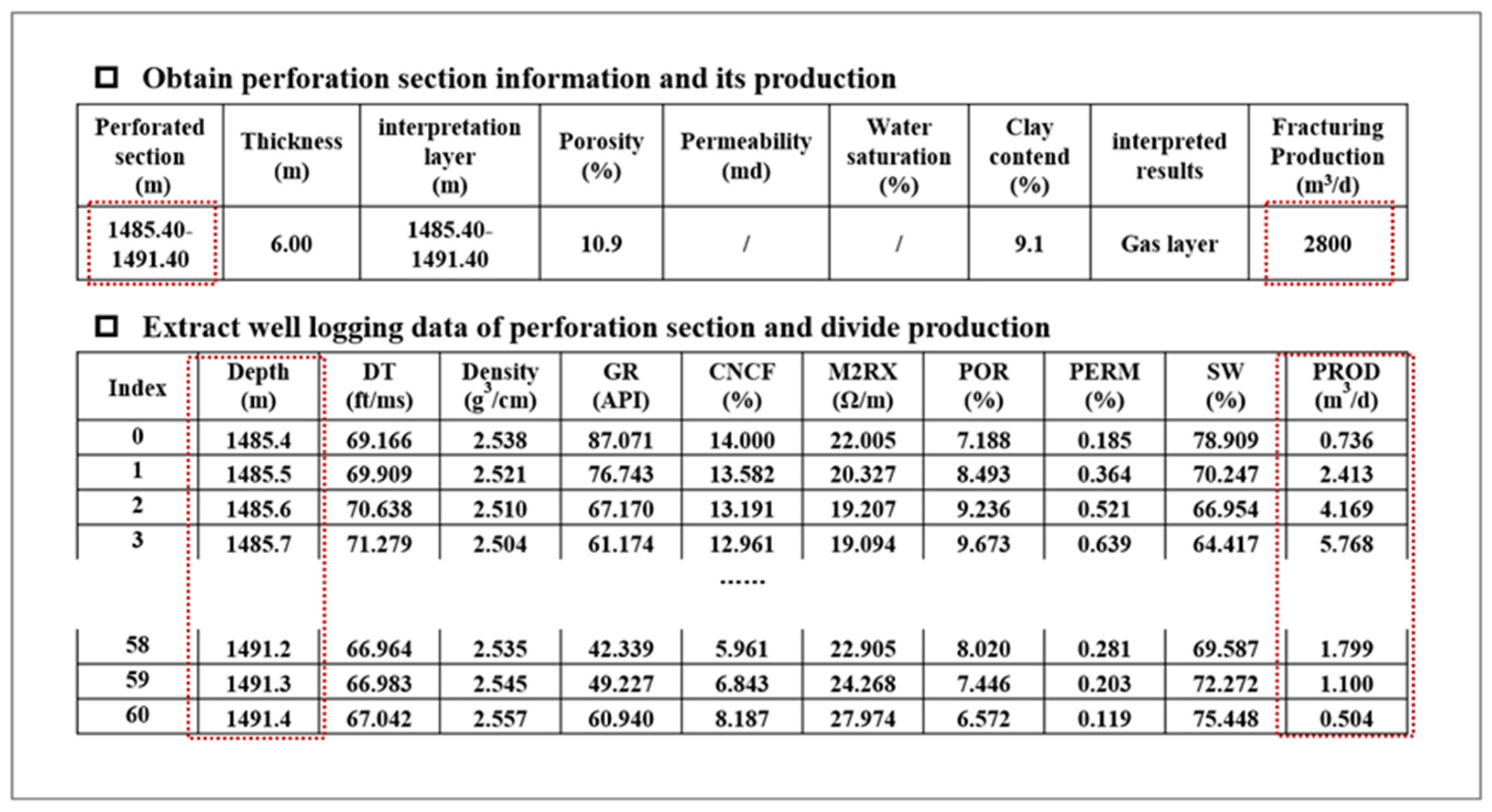
3.1. Production Segmentation
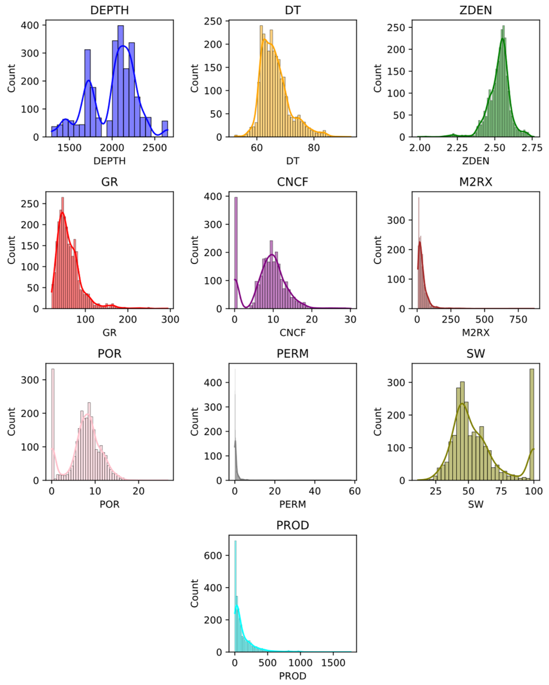
3.2. Data Description
4. Results and Discussions
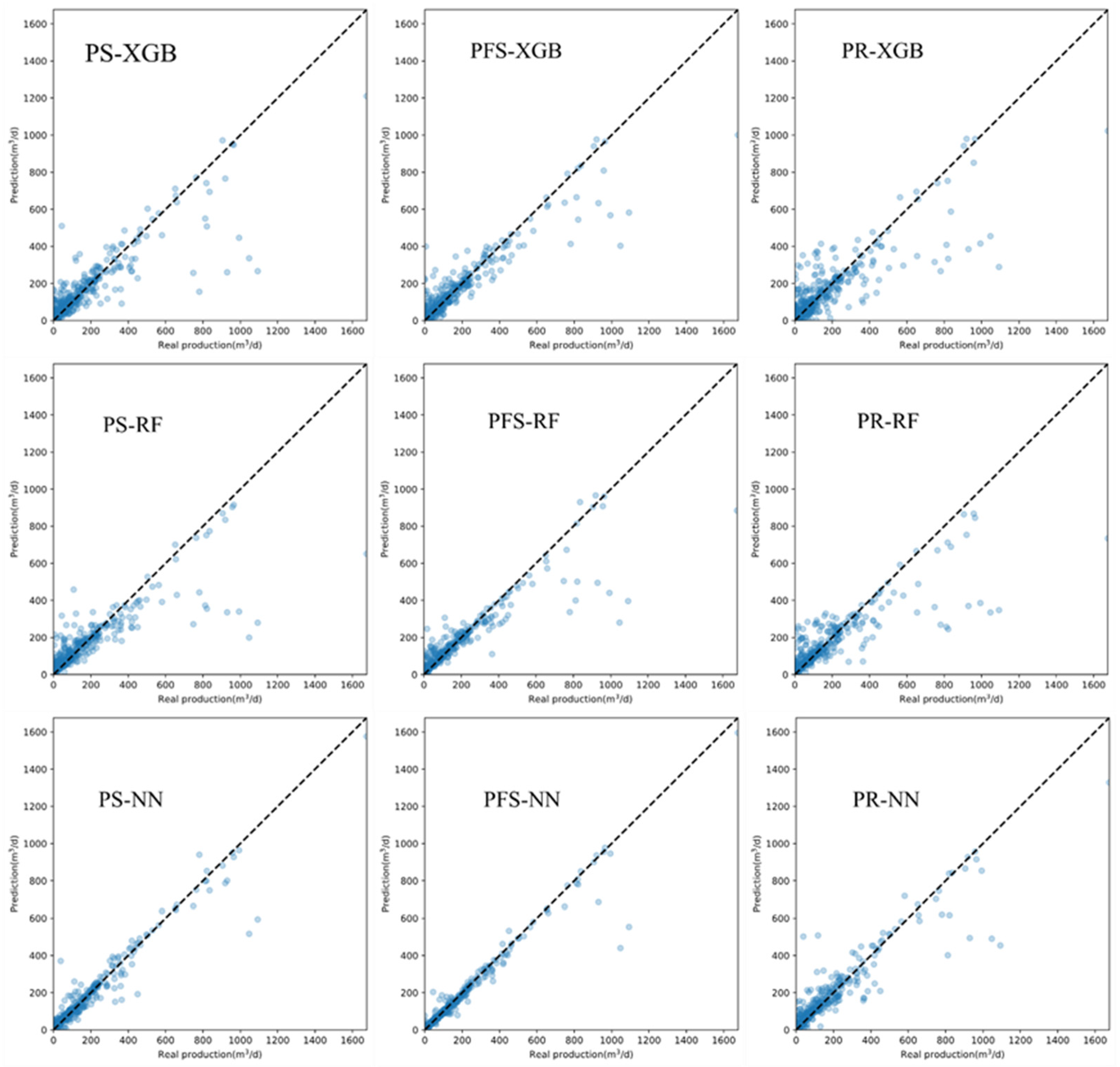
4.1. Model Performance Analysis
4.2. Comparative Analysis of PS-XGB vs. PS-RF vs. PS-NN
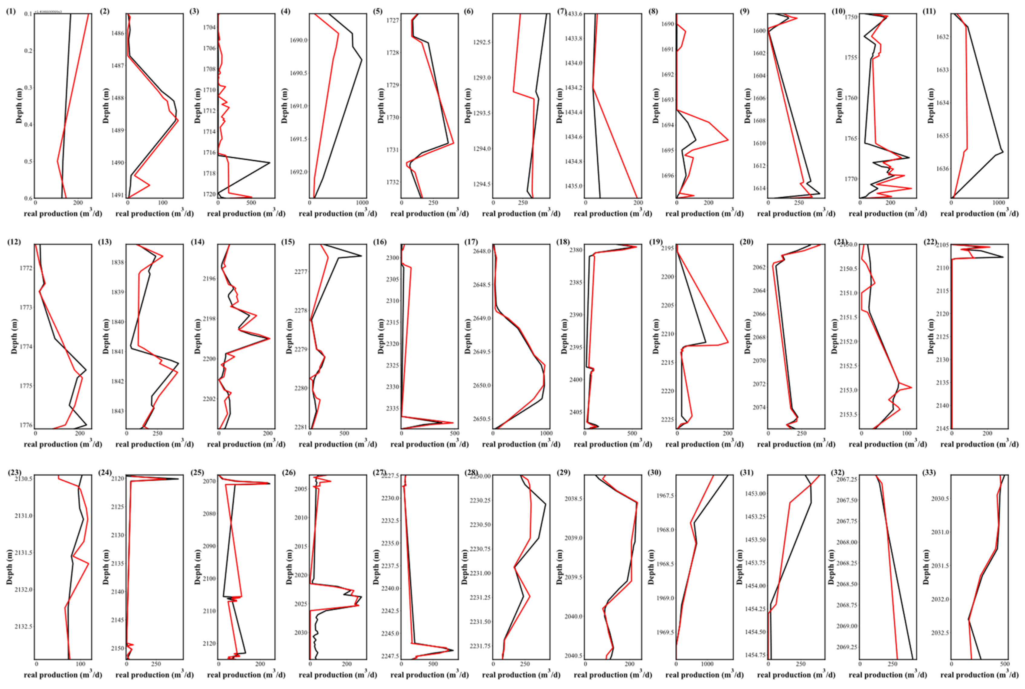
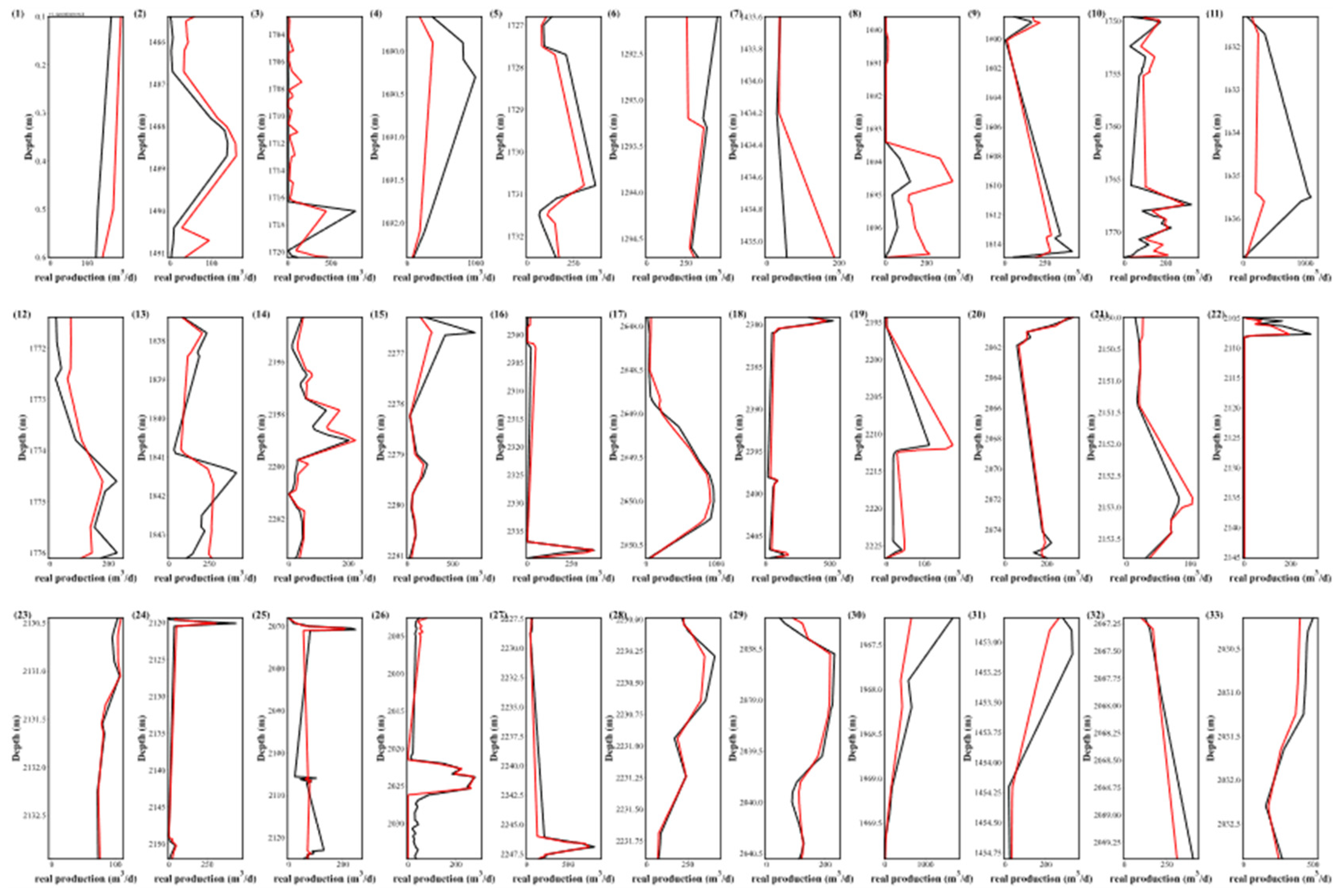
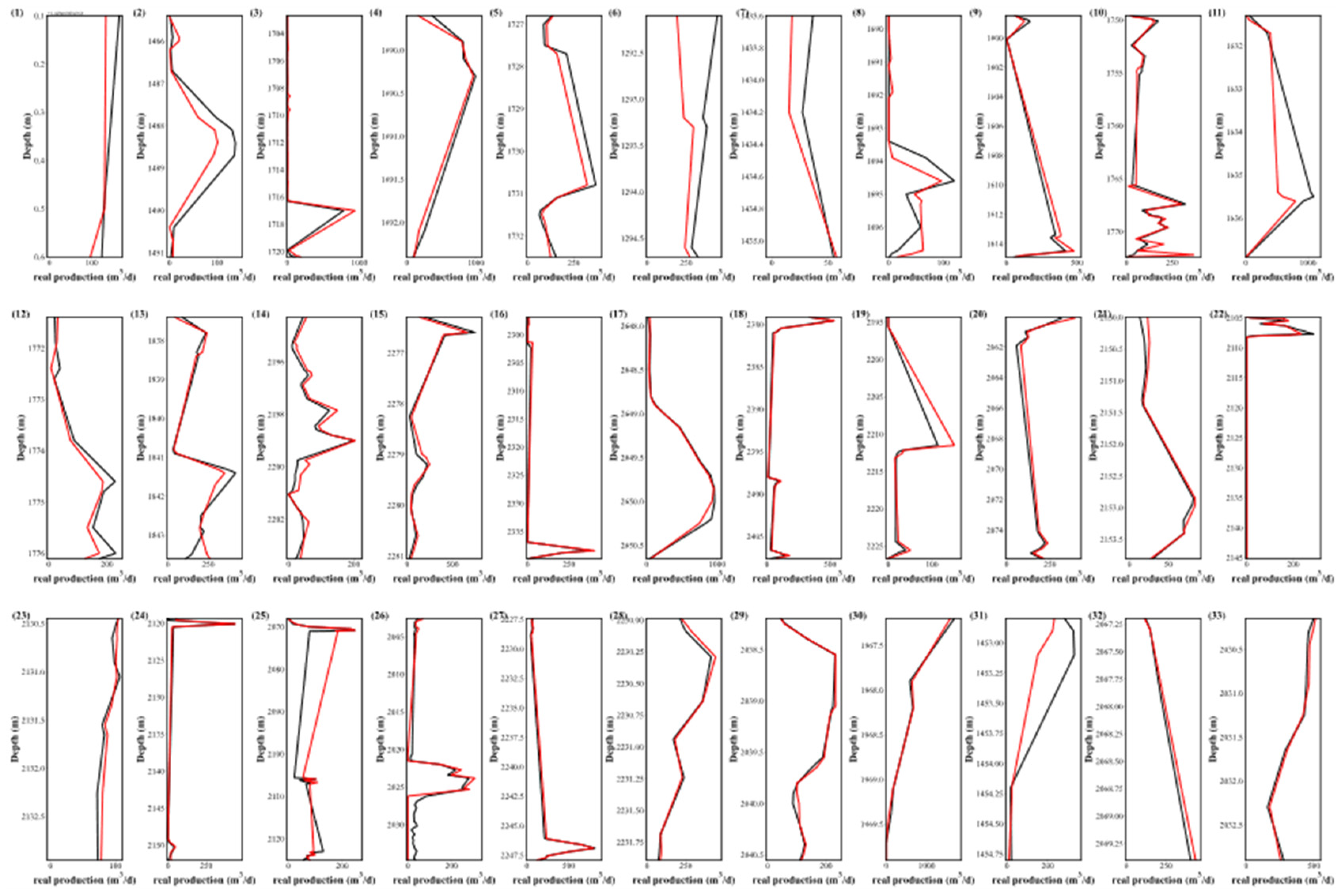
4.3. Comparative Analysis of PS-XGB vs. PFS-RF vs. PFS-NN
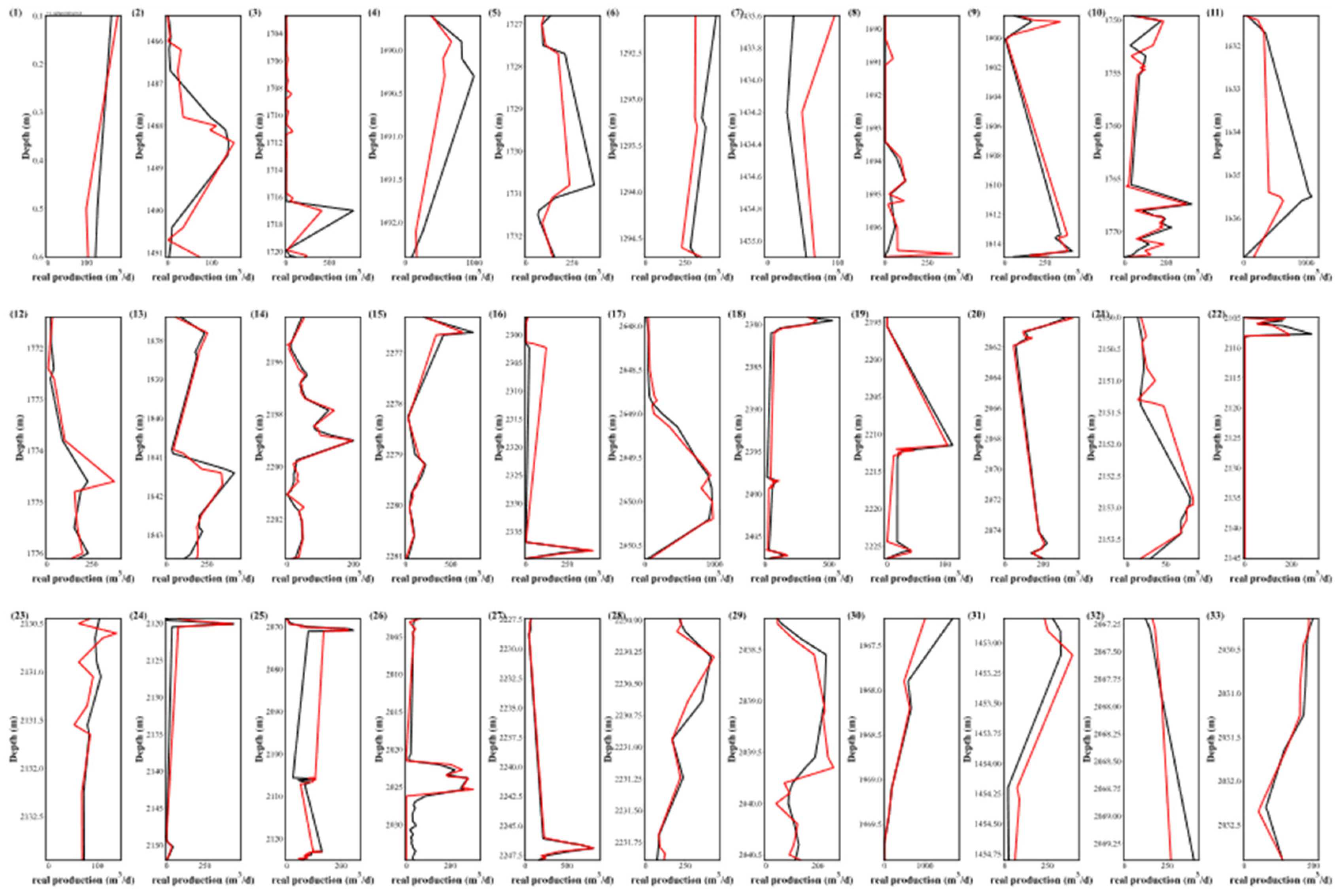
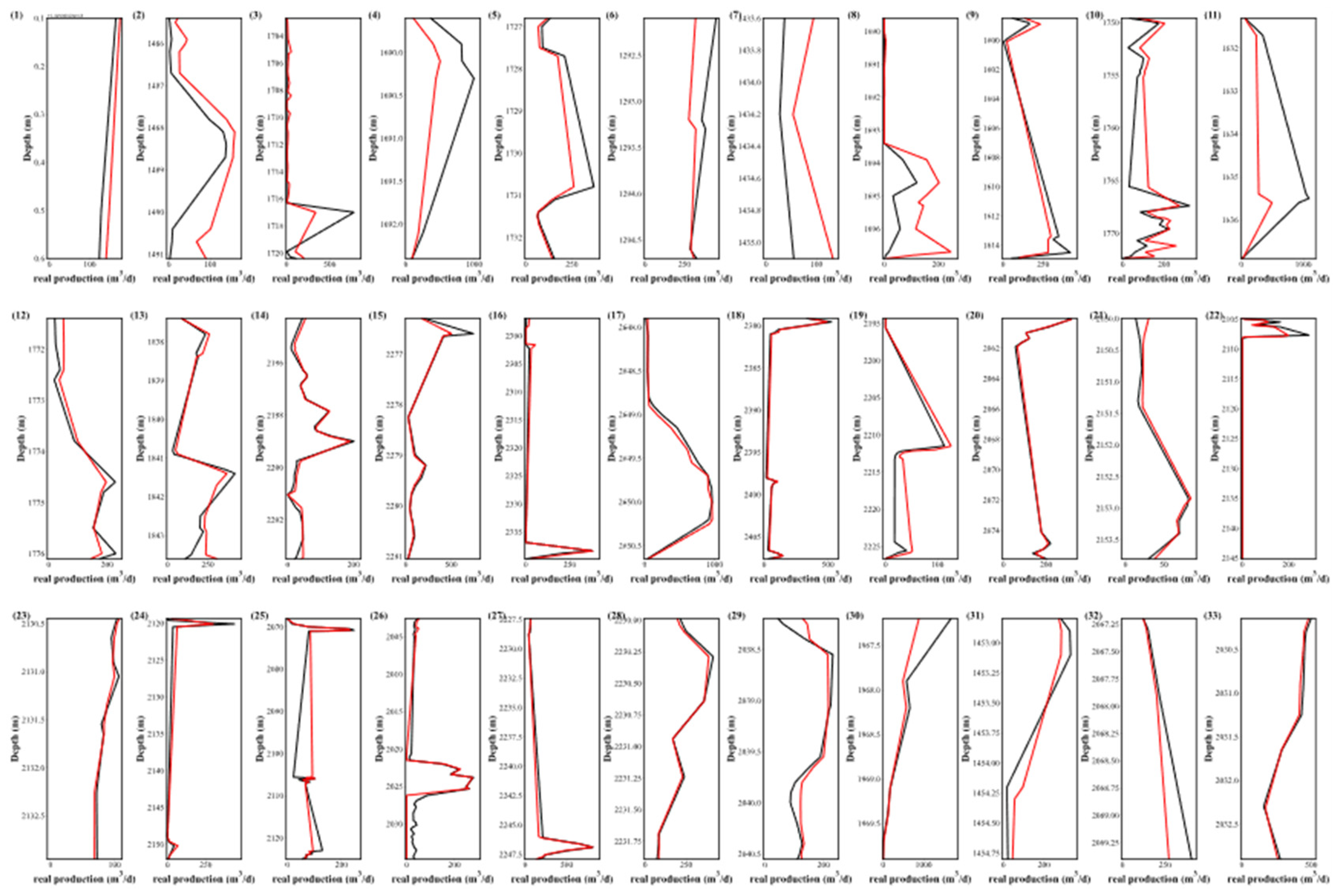
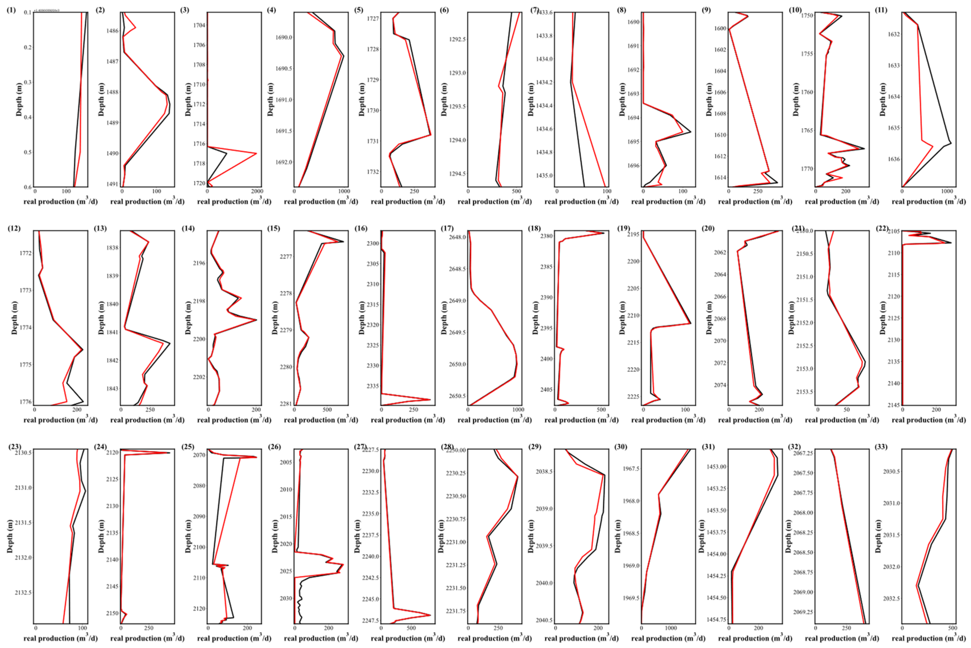
4.4. Comparative Analysis of PR-XGB vs. PR-RF vs. PR-NN
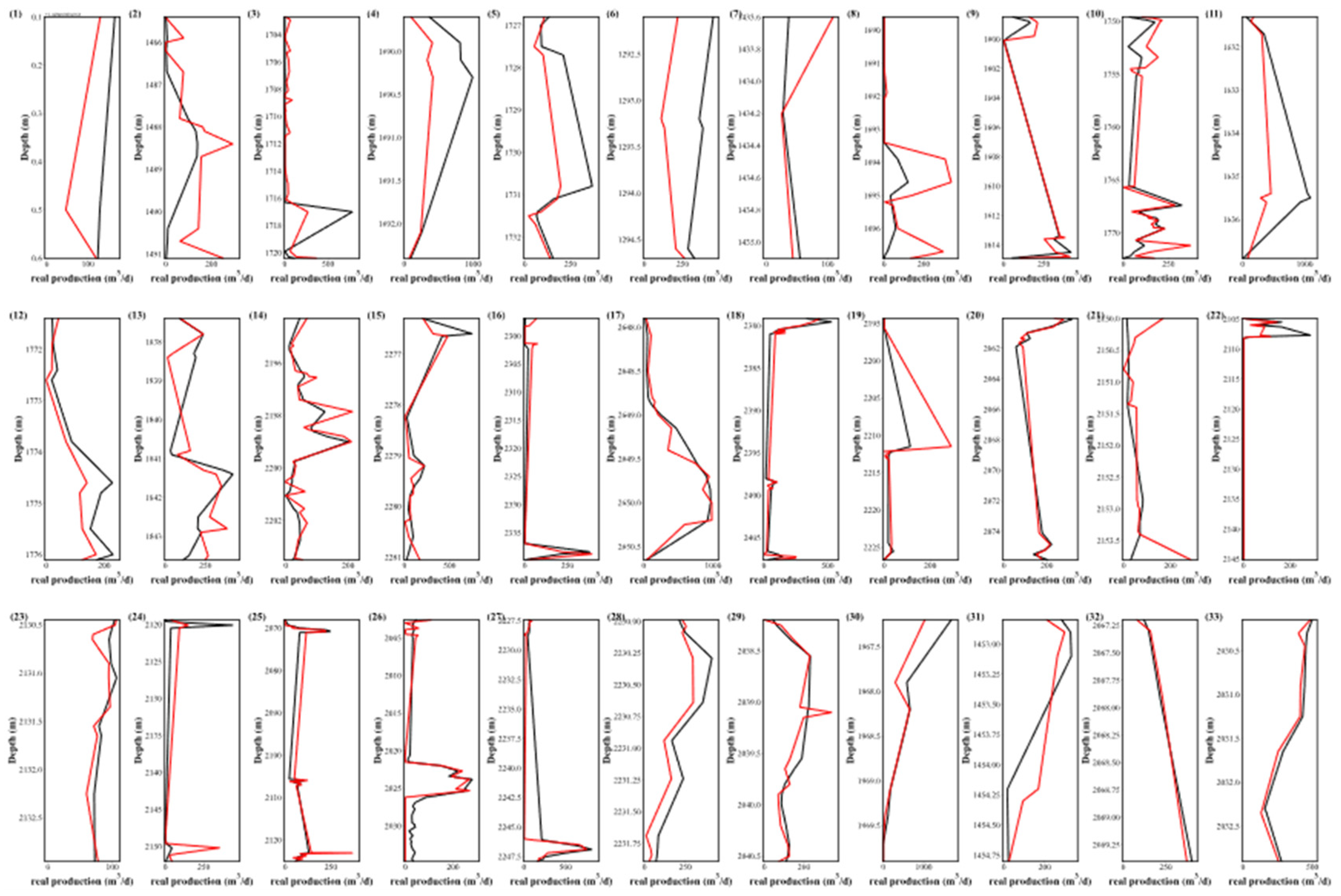
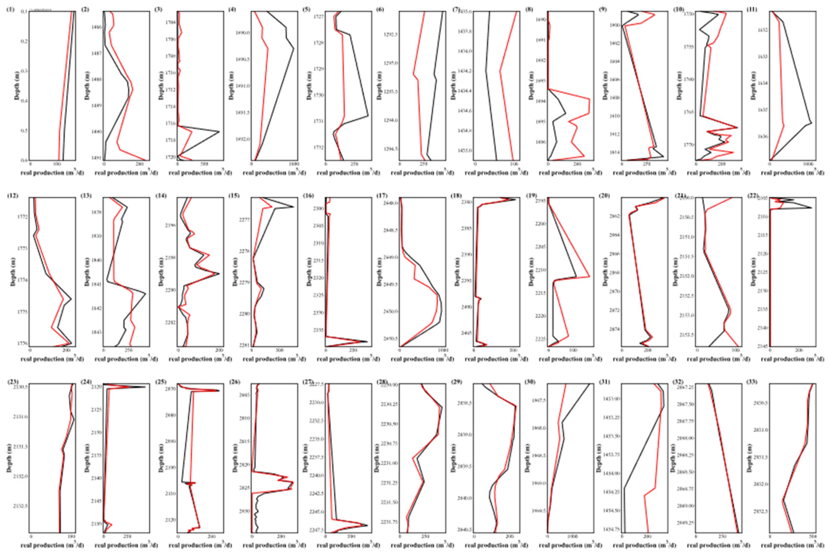
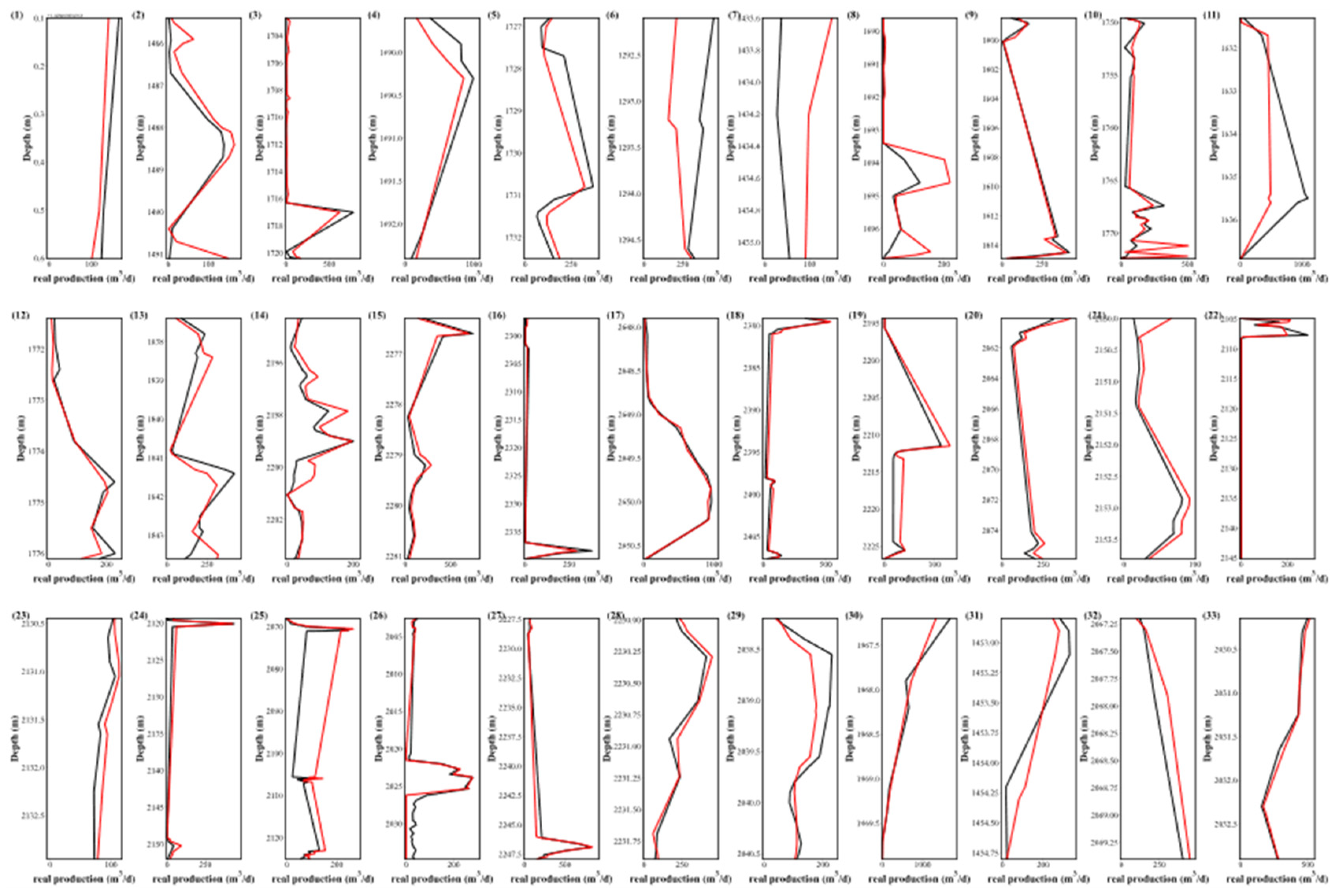
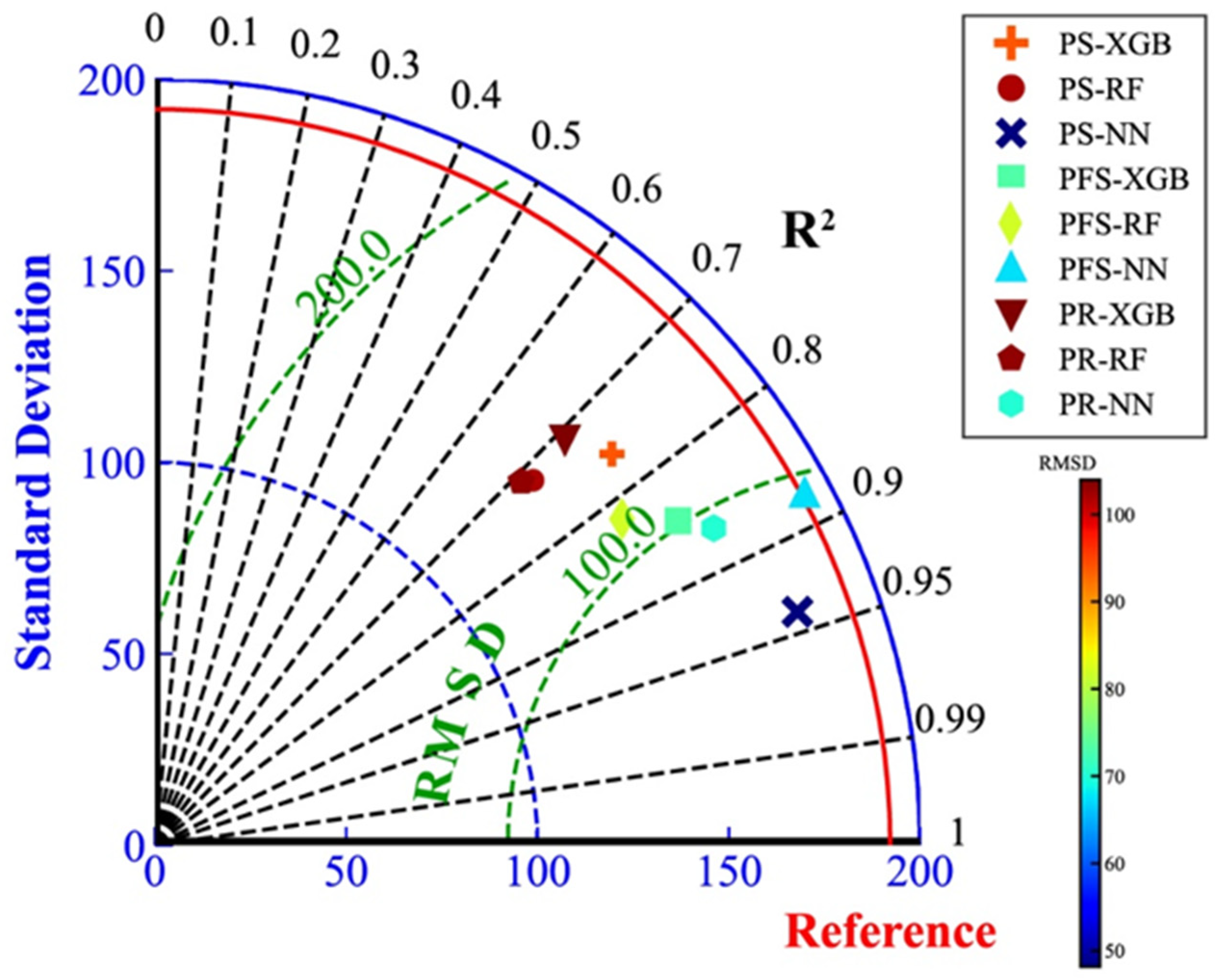
4.5. Correlation coefficient comparison
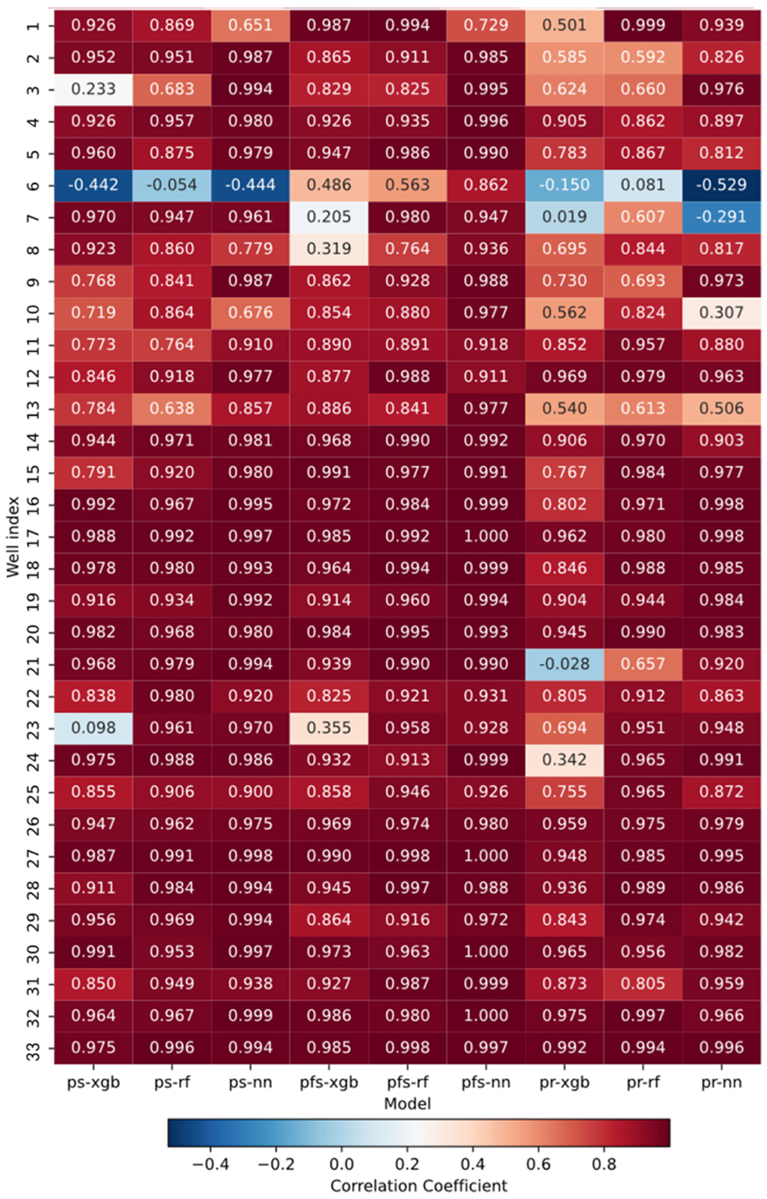
5. Conclusion
- After extensive hyperparameter tuning, it became evident that logging parameters can indeed correlate with productivity, and the prediction trends are generally on point. As such, this approach holds promise as a surrogate model for reservoir numerical simulations;
- Segmenting post-fracturing production based on well logging data at different depths is instrumental in maximizing the sample size for data-driven production predicting;
- In the context of oil and gas extraction from low-permeability and low-porosity formations, machine learning models offer an intuitive representation of the productivity distribution in relation to well depth. This is pivotal in guiding the selection of the most suitable fracturing stage during field operations. And this approach provides reservoir engineers an efficient way in reservoir performance oversight.
Nomenclature
| the original dataset | |
| the mean of the dataset | |
| the standard deviation of the dataset | |
| the formation pressure, MPa | |
| the processed value | |
| a value from the original dataset | |
| the median of the dataset | |
| the interquartile range of the dataset | |
| the prediction of the i-th instance at the t-th iteration | |
| the prediction of the k-th tree for instance xi | |
| the leaf weight assigned to the i-th instance when it reaches a leaf in the tree | |
| the function mapping an instance to the corresponding leaf in the tree | |
| the objective is a sum of a loss term (how well the model predicts) and a regularization term (to keep the model simple) | |
| the loss function that measures the difference between the true label and the predicted label for the i-th instance at the t-th iteration | |
| the first order gradient statistics of the loss function with respect to the prediction from the previous iteration | |
| he second order gradient statistics of the loss function with respect to the prediction from the previous iteration | |
| regularization term for the k-th tree | |
| the k-th real production, m3/d | |
| the k-th predicted production, m3/d | |
| the k-th real production, m3/d | |
| the mean predicted production of all wells, m3/d | |
| the standard deviation of pipelines real production, m3/d | |
| the standard deviation of pipelines predicted production, m3/d | |
| the total count of specimens | |
| the gas production of a sampling point after segmenting, m3/d | |
| the total gas production, m3/d | |
| permeability, md | |
| oil saturation, % | |
| porosity, % |
References
- Amineh M P, Yang G. China’s geopolitical economy of energy security: a theoretical and conceptual exploration[J]. African and Asian studies, 2018, 17(1-2): 9-39. [CrossRef]
- Tang, J., Wang, X., Du, X., et al. 2023. Optimization of Integrated Geological-engineering Design of Volume Fracturing with Fan-shaped Well Pattern. Petroleum Exploration and Development. 50(4): 1-8. [CrossRef]
- Tang, J., Wu, K., Zuo, L., et al. 2019. Investigation of Rupture and Slip Mechanisms of Hydraulic Fracture in Multiple-layered Formation. SPE Journal. 24(05): 2292-2307. [CrossRef]
- Huang L, Jiang P, Zhao X, et al. A modeling study of the productivity of horizontal wells in hydrocarbon-bearing reservoirs: effects of fracturing interference[J]. Geofluids, 2021, 2021: 1-13. [CrossRef]
- Zhao, X., Jin, F., Liu, X., et al. 2022. Numerical study of fracture dynamics in different shale fabric facies by integrating machine learning and 3-D lattice method: A case from Cangdong Sag, Bohai Bay basin, China. Journal of Petroleum Science and Engineering. 218: 110861. [CrossRef]
- Li, Y., Li, Z., Shao, L., et al. 2023. A new physics-informed method for the fracability evaluation of shale oil reservoirs. Coal Geology & Exploration. 51(10): 1−15. [CrossRef]
- Yang C, Bu S, Fan Y, et al. Data-driven prediction and evaluation on future impact of energy transition policies in smart regions[J]. Applied Energy, 2023, 332: 120523. [CrossRef]
- Parvizi H, Rezaei-Gomari S, Nabhani F. Robust and flexible hydrocarbon production forecasting considering the heterogeneity impact for hydraulically fractured wells[J]. Energy & Fuels, 2017, 31(8): 8481-8488. [CrossRef]
- Niu W, Lu J, Sun Y. A production prediction method for shale gas wells based on multiple regression[J]. Energies, 2021, 14(5): 1461. [CrossRef]
- Luo S, Ding C, Cheng H, et al. Estimated ultimate recovery prediction of fractured horizontal wells in tight oil reservoirs based on deep neural networks[J]. Advances in Geo-Energy Research, 2022, 6(2): 111-122. [CrossRef]
- Noshi C I, Eissa M R, Abdalla R M. An intelligent data driven approach for production prediction[C]//Offshore Technology Conference. OnePetro, 2019.
- Li X, Ma X, Xiao F, et al. A physics-constrained long-term production prediction method for multiple fractured wells using deep learning[J]. Journal of Petroleum Science and Engineering, 2022, 217: 110844. [CrossRef]
- Hongliang W, Longxin M U, Fugeng S H I, et al. Production prediction at ultra-high water cut stage via Recurrent Neural Network[J]. Petroleum Exploration and Development, 2020, 47(5): 1084-1090. [CrossRef]
- Cheng B, Tianji X U, Shiyi L U O, et al. Method and practice of deep favorable shale reservoirs prediction based on machine learning[J]. Petroleum Exploration and Development, 2022, 49(5): 1056-1068. [CrossRef]
- Hou L, Zou C, Yu Z, et al. Quantitative assessment of the sweet spot in marine shale oil and gas based on geology, engineering, and economics: A case study from the Eagle Ford Shale, USA[J]. Energy Strategy Reviews, 2021, 38: 100713. [CrossRef]
- Tang J, Fan B, Xiao L, et al. A new ensemble machine-learning framework for searching sweet spots in shale reservoirs[J]. SPE Journal, 2021, 26(01): 482-497. [CrossRef]
- Ren L, Su Y, Zhan S, et al. Progress of the research on productivity prediction methods for stimulated reservoir volume (SRV)-fractured horizontal wells in unconventional hydrocarbon reservoirs[J]. Arabian Journal of Geosciences, 2019, 12: 1-15. [CrossRef]
- Wu Y, Tahmasebi P, Lin C, et al. A comprehensive study on geometric, topological and fractal characterizations of pore systems in low-permeability reservoirs based on SEM, MICP, NMR, and X-ray CT experiments[J]. Marine and Petroleum Geology, 2019, 103: 12-28. [CrossRef]
- Huang H, Sun W, Ji W, et al. Effects of pore-throat structure on gas permeability in the tight sandstone reservoirs of the Upper Triassic Yanchang formation in the Western Ordos Basin, China[J]. Journal of Petroleum Science and Engineering, 2018, 162: 602-616. [CrossRef]
- Pimanov V, Lukoshkin V, Toktaliev P, et al. On a workflow for efficient computation of the permeability of tight sandstones[J]. arXiv preprint arXiv:2203.11782, 2022. [CrossRef]
- Ucar E, Berre I, Keilegavlen E. Three-dimensional numerical modeling of shear stimulation of fractured reservoirs[J]. Journal of Geophysical Research: Solid Earth, 2018, 123(5): 3891-3908. [CrossRef]
- Shen L, Cui T, Liu H, et al. Numerical simulation of two-phase flow in naturally fractured reservoirs using dual porosity method on parallel computers: numerical simulation of two-phase flow in naturally fractured reservoirs[C]//Proceedings of the International Conference on High Performance Computing in Asia-Pacific Region. 2019: 91-100.
- Kuhlman K L, Malama B, Heath J E. Multiporosity flow in fractured low-permeability rocks[J]. Water Resources Research, 2015, 51(2): 848-860. [CrossRef]
- van der Linden J H, Jönsthövel T B, Lukyanov A A, et al. The parallel subdomain-levelset deflation method in reservoir simulation[J]. Journal of Computational Physics, 2016, 304: 340-358. [CrossRef]
- Ucar E, Berre I, Keilegavlen E. Three-dimensional numerical modeling of shear stimulation of fractured reservoirs[J]. Journal of Geophysical Research: Solid Earth, 2018, 123(5): 3891-3908.Xin L, CA S M, Liang Z, et al. Microscale crack propagation in shale samples using focused ion beam scanning electron microscopy and three-dimensional numerical modeling. Petroleum Science, 2022.
- Pimanov V, Lukoshkin V, Toktaliev P, et al. On a workflow for efficient computation of the permeability of tight sandstones[J]. arXiv preprint arXiv:2203.11782, 2022. [CrossRef]
- Liu W, Chen Z, Hu Y, et al. A systematic machine learning method for reservoir identification and production prediction[J]. Petroleum Science, 2023, 20(1): 295-308. [CrossRef]
- Li. J., Wang, T., Wang, J., et al. 2023. Machine-Learning Proxy-based Fracture Production Dynamic Inversion with Application to Coal-bed Methane Gas Reservoir Development. Well Logging Technology.
- Ramos-Carreño C, Torrecilla J L, Carbajo-Berrocal M, et al. scikit-fda: a Python package for functional data analysis[J]. arXiv preprint arXiv:2211.02566, 2022. [CrossRef]
- Yang C, Brower-Sinning R A, Lewis G, et al. Data leakage in notebooks: Static detection and better processes[C]//Proceedings of the 37th IEEE/ACM International Conference on Automated Software Engineering. 2022: 1-12.
- Schoenfeld B, Giraud-Carrier C, Poggemann M, et al. Preprocessor selection for machine learning pipelines[J]. arXiv preprint arXiv:1810.09942, 2018. [CrossRef]
- Jamieson K, Talwalkar A. Non-stochastic best arm identification and hyperparameter optimization[C]//Artificial intelligence and statistics. PMLR, 2016: 240-248.
- Bergstra J, Bengio Y. Random search for hyper-parameter optimization[J]. Journal of machine learning research, 2012, 13(2).
- Li L, Jamieson K, DeSalvo G, et al. Hyperband: A novel bandit-based approach to hyperparameter optimization[J]. The journal of machine learning research, 2017, 18(1): 6765-6816.
- Huang. L., Qi, Y., Chen, W., et al. 2023. Geomechanical Modeling of Cluster Wells in Shale Oil Reservoirs using GridSearchCV. Well Logging Technology.
- Standardscaler S P. Available online: https://scikit-learn. org/stable/modules/generated/sklearn. preprocessing[J]. StandardScaler. html (accessed on 20 May 2022).
- BUITINCK L, LOUPPE G, BLONDEL M, et al. RobustScaler: Scikit-Learn Documentation[J]. 2018.
- Chen T, Guestrin C. Xgboost: A scalable tree boosting system[C]//Proceedings of the 22nd acm sigkdd international conference on knowledge discovery and data mining. 2016: 785-794.
- Breiman, L. (2001). Random Forests. Machine Learning, 45(1), 5–32. [CrossRef]
- Roubícková, A., MacGregor, L., Brown, N., Brown, O. T., & Stewart, M. (2020). Using machine learning to reduce ensembles of geological models for oil and gas exploration. Retrieved from http://arxiv.org/abs/2010.08775v1.
- Chang P. Multi-Layer Perceptron Neural Network for Improving Detection Performance of Malicious Phishing URLs Without Affecting Other Attack Types Classification[J]. arXiv preprint arXiv:2203.00774, 2022. [CrossRef]
- Liu T. MLPs to Find Extrema of Functionals[J]. arXiv preprint arXiv:2007.00530, 2020. [CrossRef]
- Zhu Z, Zhao J, Mu T, et al. MC-MLP: Multiple Coordinate Frames in all-MLP Architecture for Vision[J]. arXiv preprint arXiv:2304.03917, 2023. [CrossRef]
- Tran D T, Kiranyaz S, Gabbouj M, et al. Heterogeneous multilayer generalized operational perceptron[J]. IEEE transactions on neural networks and learning systems, 2019, 31(3): 710-724. [CrossRef]
- Ravanbakhsh S. Universal equivariant multilayer perceptrons[C]//International Conference on Machine Learning. PMLR, 2020: 7996-8006.
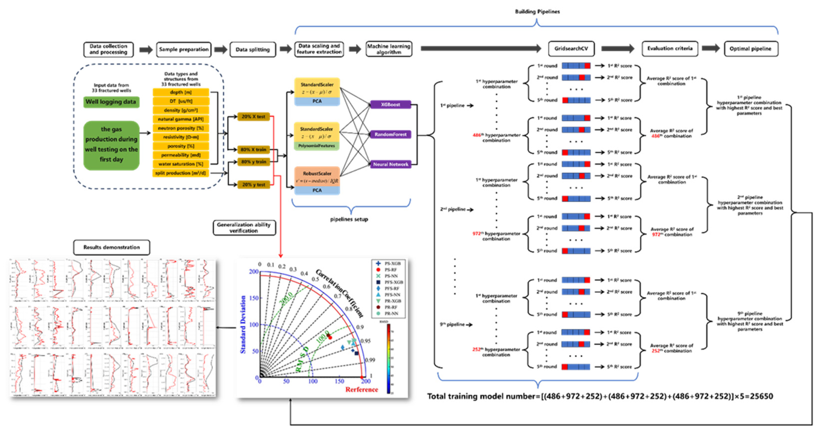
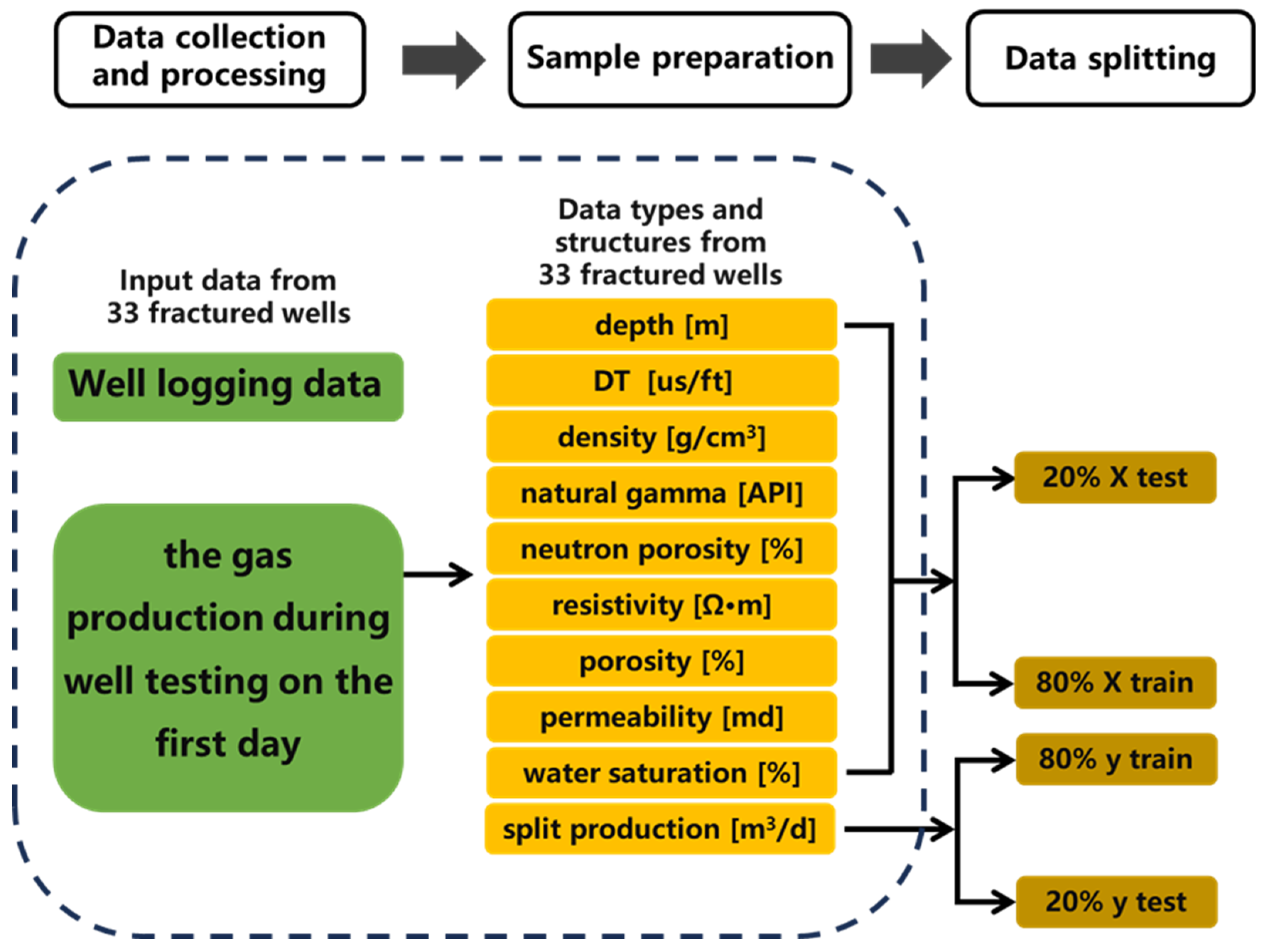
| Pipelines setup | Pipelines abbreviation |
|---|---|
| Standardscaler + PCA + XGBoost | PS-XGB |
| Standardscaler + PCA + RandomForest | PS-RF |
| Standardscaler + PCA + Neural Network | PS-NN |
| Standardscaler + PolynomialFeatures + XGBoost | PFS-XGB |
| Standardscaler+ PolynomialFeatures + RandomForest | PFS-RF |
| Standardscaler + PolynomialFeatures + Neural Network | PFS-NN |
| Robustscaler + PCA + XGBoost | PR-XGB |
| Robustscaler + PCA + RandomForest | PR-RF |
| Robustscaler + PCA + Neural Network | PR-NN |
| Pipeline | Method | Hyperparameter | Range of values |
|---|---|---|---|
| PS-XGB | PCA | n_components | 2/4/6 |
| XGBoost | learning_rate | 0.01/0.1/0.5 | |
| n_estimators | 50/100/200 | ||
| max_depth | 1/2/3 | ||
| min_child_weight | 1/3/5 | ||
| booster | 'gbtree'/'gblinear' | ||
| PS-RF | PCA | n_components | 2/4/6 |
| Random Forest | n_estimators | 400/500/600 | |
| max_depth | 2/6/10 | ||
| min_samples_split | 10/15/20 | ||
| min_samples_leaf | 4/6/8 | ||
| max_features | 'auto'/'sqrt' | ||
| bootstrap | True/False | ||
| PS-NN | PCA | n_components | 2/4/6 |
| Neural Network | hidden_layer_sizes | (50,), (100,), (200,), (100, 50), (200, 100), (300, 200, 100), (400, 300, 200, 100) | |
| alpha | 0.0001/0.001/0.01/0.1 | ||
| max_iter | 3000/5000/7000 | ||
| PFS-XGB | Polynomial Features | poly_degree | 2/3/4 |
| XGBoost | learning_rate | 0.01/0.1/0.5 | |
| n_estimators | 50/100/200 | ||
| max_depth | 1/2/3 | ||
| min_child_weight | 1/3/5 | ||
| booster | 'gbtree'/'gblinear' | ||
| PFS-RF | Polynomial Features | poly__degree | 2/3/4 |
| Random Forest | n_estimators | 400/500/600 | |
| max_depth | 2/6/10 | ||
| min_samples_split | 10/15/20 | ||
| min_samples_leaf | 4/6/8 | ||
| max_features | 'auto'/'sqrt' | ||
| bootstrap | True/False | ||
| PFS-NN | Polynomial Features | poly__degree | 2/3/4 |
| Neural Network | hidden_layer_sizes | (50,), (100,), (200,), (100, 50), (200, 100), (300, 200, 100), (400, 300, 200, 100) | |
| alpha | 0.0001/0.001/0.01/0.1 | ||
| max_iter | 3000/5000/7000 | ||
| PR-XGB | PCA | n_components | 2/4/6 |
| XGBoost | learning_rate | 0.01/0.1/0.5 | |
| n_estimators | 50/100/200 | ||
| max_depth | 1/2/3 | ||
| min_child_weight | 1/3/5 | ||
| booster | 'gbtree'/'gblinear' | ||
| PR-RF | PCA | n_components | 2/4/6 |
| Random Forest | n_estimators | 400/500/600 | |
| max_depth | 2/6/10 | ||
| min_samples_split | 10/15/20 | ||
| min_samples_leaf | 4/6/8 | ||
| max_features | 'auto'/'sqrt' | ||
| bootstrap | True/False | ||
| PR-NN | PCA | n_components | 2/4/6 |
| Neural Network | hidden_layer_sizes | (50,), (100,), (200,), (100, 50), (200, 100), (300, 200, 100), (400, 300, 200, 100) | |
| alpha | 0.0001/0.001/0.01/0.1 | ||
| max_iter | 3000/5000/7000 |
| Pipeline | Hyperparameter | The best of values |
|---|---|---|
| PS-XGB | n_components | 6 |
| learning_rate | 0.5 | |
| n_estimators | 200 | |
| max_depth | 3 | |
| min_child_weight | 5 | |
| booster | 'gbtree' | |
| PS-RF | n_components | 6 |
| n_estimators | 400 | |
| max_depth | 10 | |
| min_samples_split | 10 | |
| min_samples_leaf | 4 | |
| max_features | 'sqrt' | |
| bootstrap | False | |
| PS-NN | n_components | 6 |
| hidden_layer_sizes | (400, 300, 200, 100) | |
| alpha | 0.01 | |
| max_iter | 7000 | |
| PFS-XGB | poly_degree | 3 |
| learning_rate | 0.1 | |
| n_estimators | 200 | |
| max_depth | 3 | |
| min_child_weight | 5 | |
| booster | 'gbtree' | |
| PFS-RF | poly__degree | 3 |
| n_estimators | 500 | |
| max_depth | 10 | |
| min_samples_split | 10 | |
| min_samples_leaf | 4 | |
| max_features | 'sqrt' | |
| bootstrap | False | |
| PFS-NN | poly__degree | 2 |
| hidden_layer_sizes | (300, 200, 100) | |
| alpha | 0.0001 | |
| max_iter | 3000 | |
| PR-XGB | n_components | 6 |
| learning_rate | 0.5 | |
| n_estimators | 200 | |
| max_depth | 3 | |
| min_child_weight | 1 | |
| booster | 'gbtree' | |
| PR-RF | n_components | 6 |
| n_estimators | 600 | |
| max_depth | 10 | |
| min_samples_split | 10 | |
| min_samples_leaf | 4 | |
| max_features | 'sqrt' | |
| bootstrap | False | |
| PR-NN | n_components | 6 |
| hidden_layer_sizes | (400, 300, 200, 100) | |
| alpha | 0.01 | |
| max_iter | 3000 |
| Model | R2 | RMSE | SD |
|---|---|---|---|
| Reference | 1 | 0 | 192.2 |
| PS-XGB | 0.76 | 93.79 | 157.19 |
| PS-RF | 0.72 | 101.78 | 137.29 |
| PS-NN | 0.94 | 48.15 | 178.68 |
| PFS-XGB | 0.85 | 73.19 | 160.85 |
| PFS-RF | 0.82 | 81.86 | 148.87 |
| PFS-NN | 0.88 | 67.35 | 192.99 |
| PR-XGB | 0.71 | 103.98 | 150.94 |
| PR-RF | 0.71 | 102.93 | 134.86 |
Disclaimer/Publisher’s Note: The statements, opinions and data contained in all publications are solely those of the individual author(s) and contributor(s) and not of MDPI and/or the editor(s). MDPI and/or the editor(s) disclaim responsibility for any injury to people or property resulting from any ideas, methods, instructions or products referred to in the content. |
© 2023 by the authors. Licensee MDPI, Basel, Switzerland. This article is an open access article distributed under the terms and conditions of the Creative Commons Attribution (CC BY) license (http://creativecommons.org/licenses/by/4.0/).


