Autonomous Vehicle Decision Making with Policy Prediction for Handling a Round Intersection

Preprint

Article

Autonomous Vehicle Decision Making with Policy Prediction for Handling a Round Intersection

This version is not peer-reviewed.

This version is not peer-reviewed.

Altmetrics

Downloads

101

Views

Comments

Submitted:

22 October 2023

Posted:

24 October 2023

You are already at the latest version

A peer-reviewed article of this preprint also exists.

Abstract

Autonomous shuttles have been used as end mile solutions for smart mobility in smart cities. The urban driving conditions of smart cities with many other actors sharing the road and the presence of intersections have posed challenges to the use of autonomous shuttles. Round intersections are more challenging as it is more difficult to perceive the other vehicles in and near the intersection. Thus, this paper focuses on decision making of autonomous vehicles for handling round intersections. The round intersection is introduced first, followed by introductions of the Markov Decision Process (MDP), the Partially Observable Markov Decision Process (POMDP) and the Object Oriented Partially Observable Markov Decision Process (OOPOMDP) which are used for decision making with uncertain knowledge of the motion of the other vehicles. The Partially Observable Monte-Carlo Planning (POMCP) algorithm is used as the solution method and OOPOMDP is applied to decision making for autonomous vehicles in round intersections. Decision making is formulated first as a POMDP problem, and the penalty function is formulated and set accordingly. This is followed by improvement of decision making with policy prediction. Augmented objective state and policy-based state transition are introduced and simulations are used to demonstrate the effectiveness of the proposed method for collision free handling of round intersections by the ego vehicle.

Keywords:

Subject:

Engineering - Transportation Science and Technology

1. Introduction

Active mobility and last mile delivery are crucial aspects of urban transportation, and autonomous vehicles are increasingly being proposed and used in pilot deployments worldwide to help. Current shuttles used for solving the last mile problem have difficulty in handling intersections autonomously and the operator must check the intersection and press a proceed type button after making sure that it is safe to enter. Understanding how autonomous vehicles navigate complex intersections is essential for their safe and efficient integration into the existing transportation infrastructure. This paper, therefore, focuses on decision making for handling a round intersection with partially observable information about the motion of the other vehicles.

Self-driving or autonomous vehicles are already available in limited scale operations around the world and are expected to become more available soon [1]. When autonomous vehicles also use on-board units which are vehicular to everything communication modems, they become connected and autonomous vehicles (CAV) [2,3,4,5]. Due to their increasing availability, CAVs have been the focus of both academic and industry research and, as a result, there is lot of research on autonomous driving function controls and their higher-level decision-making algorithms. For example, reference [6] treats motion planning for autonomous vehicles driving on highways. Real time motion planning for urban autonomous vehicles is presented in [7]. A survey of autonomous vehicle common practices and emerging technologies is the topic of [8]. A survey of autonomous vehicle localization methods can be found in [9]. Robust control of path tracking is treated in [10]. Reference [11] is on path planning and control of autonomous vehicles and presents rule-based decision making. A survey of autonomous vehicle decision making at straight intersections is presented in [12].

Planning and decision making are the core functions of an autonomous vehicle for driving safely and efficiently under different traffic scenarios. As discussed in [13], the decision making and planning algorithms for autonomous vehicles aim at solving problems like: (a) determining the future path, (b) utilizing observations of the surrounding environment using the perception system, (c) acting properly when interacting with other road users, (d) instructing the low-level controller of the vehicle and (e) ensuring that autonomous driving is safe and efficient. Therefore, planning and decision making are very important for autonomous driving. Depending on the traffic scenario, autonomous driving functions are designed for highway driving, off-road driving, or urban driving. Research for highway driving and off-road driving have been going on for a long time with many results on planning and decision making. Due to the complexity of the urban traffic scenario, the decision making and planning for the urban traffic environment has always been very challenging with many unsolved problems remaining.

The complexity of the urban traffic scenario is manifested in the following aspects which are discussed next. The first problem is the presence of a large variation of road types. Roads on a highway scenario are quite similar. Vehicles should either stay in their lane or execute lane changes if needed. Unlike a highway, an urban traffic scenario is composed of different road types, including lanes, intersections, traffic circles, roundabouts as well as lanes for bicyclists and crosswalks for pedestrians. Hence, the decision making and planning need to include intersection management and driving on different types of roads including one-way ones. The second problem is the presence of many different types of road users who share the road. In an urban traffic scenario, the road users are not only vehicles, but also vulnerable road users (VRU) such as bicyclists, pedestrians, scooterists etc. It will cause much more damage when VRUs are involved in traffic accidents. The safety of driving, thus, is what the autonomous vehicle and its planning algorithm should always prioritize. Then, there are intersections which may or may not be signalized. Decision making is easier when the intersection is signalized and there are traffic lights in addition [14]. The rules of interaction in a signalized intersection with stop signs are also well established but the interpretation or lack of knowledge of these rules by drivers may make it difficult for an autonomous vehicle to handle the intersection. Handling a round intersection is always a more challenging task for an autonomous vehicle as decision making requires knowledge of the other vehicles in the intersection and prediction of their intent. This paper focuses on decision making of autonomous vehicles in round intersections and is motivated by the difficulty of autonomously handling the two round intersections by the AV shuttles of the recent Linden LEAP deployment in Columbus, Ohio, U.S.A. as part of its Smart Columbus project [15,16].

An intersection is a junction where roads meet and cross. One of the major challenges of autonomous vehicle decision making in urban traffic is handling intersections, especially round intersections that are not signalized. This paper, therefore, focuses on autonomous vehicle decision making and planning in round intersections. A round intersection is a special case of unsignalized intersections. Intersections, based on the existence of traffic signals, are usually categorized into two types: signalized intersections and unsignalized intersections. The signalized intersection is a centralized control system where the traffic flow is controlled by the traffic signal, either traffic lights or traffic signs. Thus, vehicles will behave according to the traffic signal, not requiring extra decision making or behavior planning. In contrast, at an unsignalized intersection, the decision making and planning are decided upon by the driver or the planner for an autonomous vehicle for determining their behavior when approaching the intersection as well as for interacting with other nearby road users or the traffic within the intersection zone.

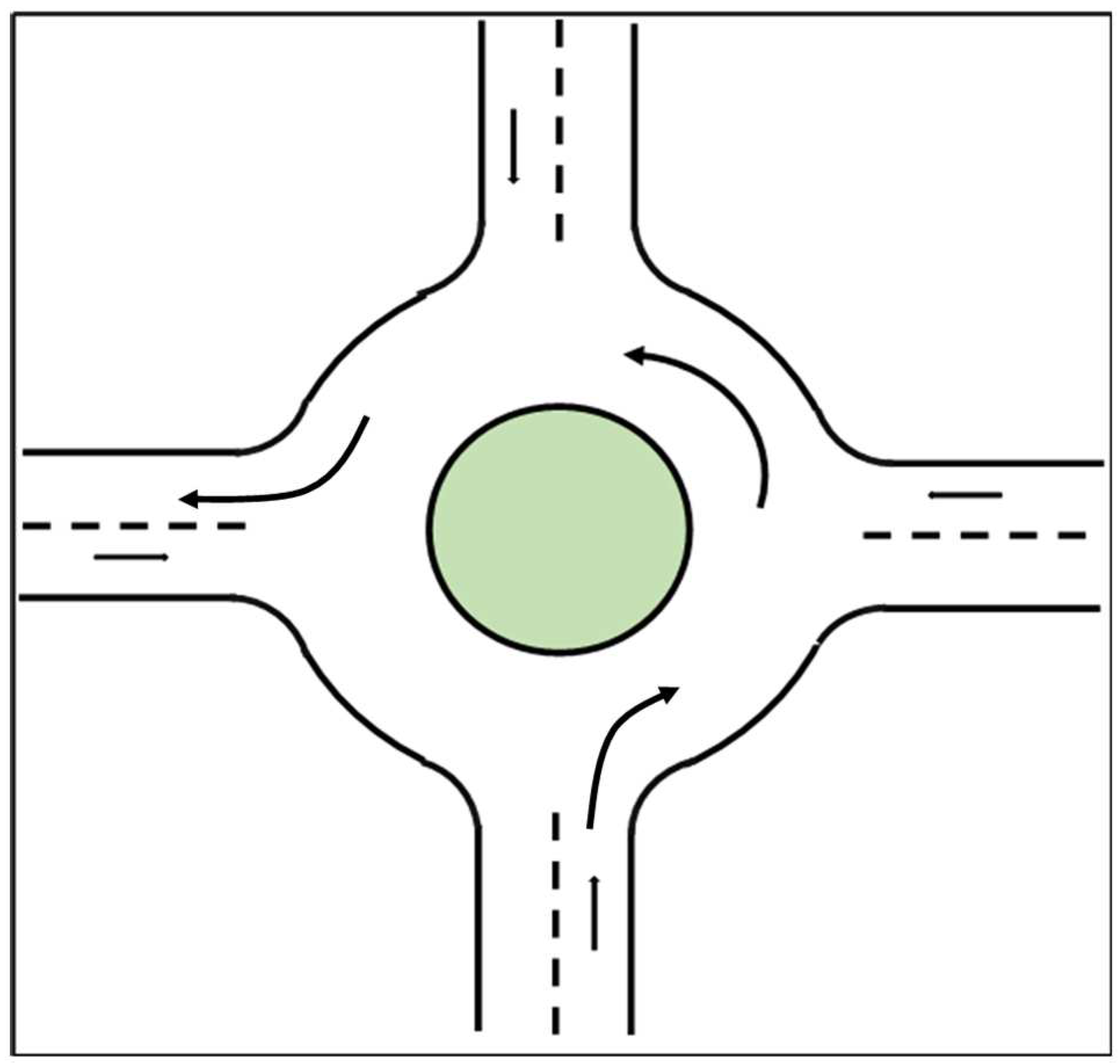
The geometric layout of the round intersection considered in this paper is shown in Figure 1 and resembles the two Linden LEAP AV shuttle route intersections in references [15,16]. The round intersection in Figure 1 can be viewed as a combination of three types of roads: the one lane straight road before the round intersection, the entry/exit part of the round intersection and the round part of the intersection where the vehicle can only drive in the counterclockwise direction. Vehicles enter the round intersection from the straight road and exit in the area of exit/entry. Vehicles will follow the straight and curved lane in straight roads and in the round intersection, respectively. For a single vehicle, the change of angular velocity in different parts of the road makes it difficult for the vehicle motion model to track the vehicle behavior. When there are multiple vehicles in the traffic scenario, the interaction between vehicles requires a good decision making and planning algorithm for the autonomous vehicle. In this paper, a decision-making algorithm based on the Partially Observable Markov Decision Making Process (POMDP) for planning the acceleration of the autonomous vehicle is proposed. A policy prediction method is also used for better tracking of trajectories of other vehicles which leads to better decision making.

The organization of the rest of the paper is as follows. The Markov Decision Process (MDP), the Partially Observable Markov Decision Process (POMDP), the Object Oriented Partially Observable Markov Decision Process (OOPOMDP) and Partially Observable Monte-Carlo Planning algorithm (POMCP) solution are introduced in Section 2. OOPOMDP is also applied to decision making for autonomous vehicles in round intersections in Section 2 where the penalty function is formulated and set. Improvement of decision making with policy prediction is presented in Section 3. The augmented objective state and policy-based state transition are introduced in Section 4. Simulations are used in Section 5 to demonstrate the effectiveness of the proposed method. The paper ends with conclusions and recommendations in the last section.

2. Decision Making and Planning for Handling Round Intersections

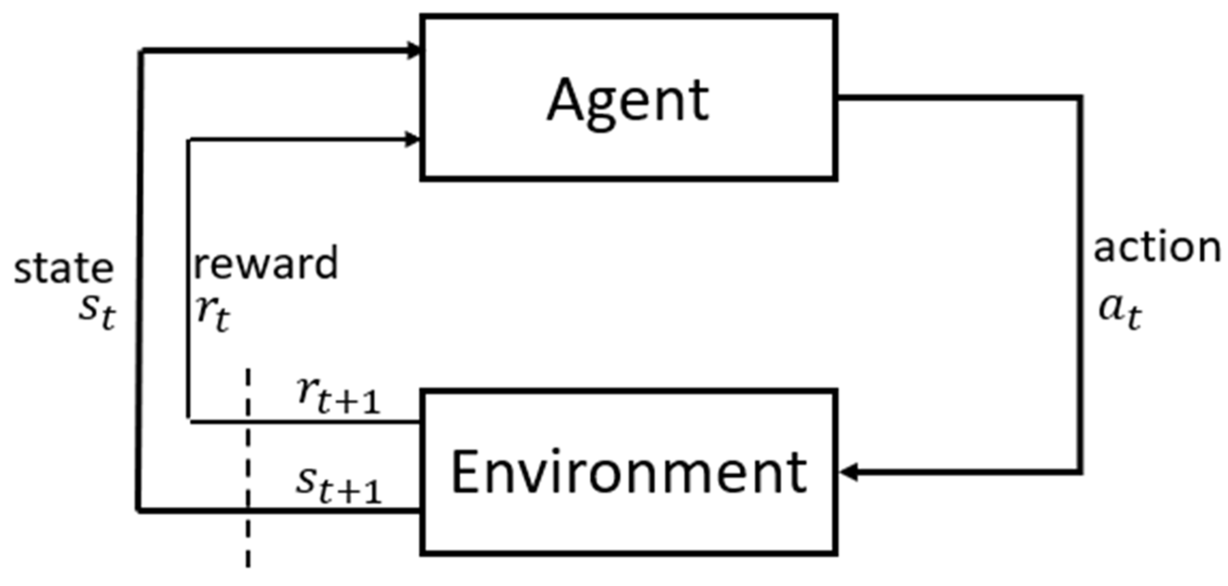
The motion planning and decision making of autonomous vehicles can be viewed as a sequential decision-making problem. The Markov Decision Process (MDP) and the Partially Observable Markov Decision Process (POMDP) represent a very wide range of methods for solving the sequential decision-making problem. In the Markov Decision Process, an agent takes actions that affect the whole system which includes the environment and the agent itself. The agent is looking for actions which lead to future maximal rewards collected from the whole system as illustrated in Figure 2.

Formally, MDP is defined by the 5-tuple

〈 S, A, T, R, γ 〉

, where

S

represents the collection of states

s

, including the states of the agent as well as uncontrollable factors in the environment. A represents the action space which is a set of executable actions that the agent can take. T is the transition model. R is the reward function with

γ

representing the discount factor. The transition model

T (s' | s, a)

denotes the probability that the system updates to state

s'

given that the system takes an action

a

at the state

s

. The reward function

R (s, a)

provides the immediate reward when the system takes an action

a

at the state

s

. The action

a

is derived from the policy function

π (s, a) = P (a | s)

, or probability of a given s, to achieve the overall optimization goal of the cumulative expected reward of

E [\sum_{t = 0}^{\infty} γ^{t} R (s_{t}, a_{t})] .

(1)

The discount factor γ reduces the effect of the reward with time. The difference of POMDP from MDP is that the system state

s

is not fully observable to the agent. Instead, the agent can only access observations that are generated probabilistically, based on the action and the possible true states. The PODMP can be represented as a 7-tuple extended from MDP as

〈 S, A, T, R, O, Z, γ 〉

where

S, A, T, R

and

γ

have the same meanings as in an MDP. Of the two additional elements,

O

represents the observation space which contains observations

o

that the agent perceives from the system and the environment and

Z

is the observation model with

Z (o | s', a, s)

denoting the probability or probability density of receiving observation

o

in state

s'

given the previous state and action were

s, a

, respectively.

The distinction between POMDP and MDP is that the agent does not have a full knowledge of the environment and the system. Hence, the state information must be inferred from the entire history of previous actions and observations as well as the initial belief information

b_{0}

. The policy is now a mapping from history to an action. The history at time t is denoted as

h_{t} = {b_{0}, a_{0}, o_{1}, a_{1}, o_{2}, ..., a_{t - 1}, o_{t}}

. As a contrast, the policy mapping function now depends on the history rather than the states themselves,

π (h_{t}, a) = P (a | h_{t})

. Due to the lack of knowledge of state

s

, the belief state which is the probability distribution over states given the history is introduced as

b (s) = \Pr (s_{t} | h_{t} = h)

(2)

which is important for the POMDP for updating the belief states. After reaching a new state

s'

, the agent observes a new observation

o

based on the observation model. The belief update rule for POMDP is

b' (s') = η Z (o | s', a) \sum_{s \in S} T (s' | s, a) b (s)

(3)

The overall optimization is refined as

a^{*} = \arg \max_{a_{t}} E [\sum_{t = 0}^{\infty} γ^{t} R (s_{t}, a_{t}) | b_{0}]

(4)

In the case of the autonomous driving decision making problem, the ego-vehicle does not have full observation over other vehicles or road user states. Hence, POMDP provides a better method for solving the sequential decision-making problem for autonomous driving under uncertainties and partial observability.

Traditional POMDP works well for problems with a state space which is of small domain and low dimension. However, POMDP becomes computationally intractable for planning over large domain and results in the “curse of dimensionality” issue for its solution [17]. Since the state space is not fully observable for the agent, the agent needs to develop a belief representation over the state space which grows exponentially with the number of the state variables. As for the decision-making problem of autonomous vehicle driving, the number of other vehicles in the environment will normally be large, and the decision horizon can be long to finish a driving task in specific traffic scenarios. Both of these factors in a traffic scenario will lead to the large domain for the POMDP problem.

To improve the performance and deal with the intractability of POMDP over a large domain, an Object-Oriented POMDP was proposed in [18] for solving a multi-object search task. It is also useful when applied to solving autonomous driving decision making problems due to the large domains in the problem formulation of a traffic scenario with multiple vehicles in it. Object-Oriented POMDP (OOPOMDP) provides an extension for POMDPs by factorizing both state and observation spaces in terms of object. It uses object state abstractions to enable the agent to reason about objects and relations between objects. The OOPOMDP problem can be represented as an 11-tuple

〈 C, A t t (c), D o m (a), O b j, S, A, T, R, Z, O, γ 〉

. In this notation, the

S, A, T, R, O, Z

and

γ

have the same meanings as those in the POMDP problems. However, in the problem of OOPOMDP, a new set

O b j

is introduced.

O b j = {o b j_{1}, ..., o b j_{n}}

is a set that the state space

S

and observation space

O

are factored into. Each

O b j_{i}

is an instance of a particular class,

c \in C

. Those classes have their class specific attribute that are defined in the set

A t t (c)

D o m (a)

defines the possible values of each attribute in the attribute set. The dual factorization of S and

O

allows the observation functions to exploit shared structure to define observations grounded in the state with varying degrees of specificity: over a class of objects, a single object, or an object’s attribute.

One of the important steps in solving a POMDP that causes the problem of “curse of dimensionality” is the belief update procedure, as given by Equation (3). The belief state over possible state space has to be updated according to the transition and observation models. The state space grows exponentially along the update of the belief space regarding the number of objects. Assume that there are

M

possible states for the

N

objects in the current decision region. Then, the states to be covered by the POMDP are:

| S | = \prod_{i = 1}^{N} | S_{o b j_{i}} | = | M |^{N}

(5)

Therefore, the dimension of the belief state

b (s)

also grows exponentially with the state space.

The OOPOMDP method improves the step for belief update over multiple objects and reduces the dimension of states by exploring one possible independence assumption. When assuming that objects in the environment are independent from each other, the belief state over the state space can be viewed as a union of belief states over the state of each object as

\begin{array}{l} b (s) = b (\cup_{i = 1}^{N} s_{i}) = b (s_{1}) b (s_{2}) ... b (s_{N}) \\ = \prod_{i = 1}^{N} b (s_{i}) \end{array}

(6)

Thus, the exponentially growing belief state now scales linearly in the number of objects

N

in the environment. The dimension of the unfactored belief, which are the beliefs that are not processed by the OOPOMDP, is

| M |^{N}

. While the dimension of the factored belief state is

N | M |

. When providing object-specific observation

o_{i}

with respect to each of the independent objects in the environment, the belief update can also be object-specific for object i as

b_{i}^{'} (s_{i}) = η p (o_{i} | s_{i}) b_{i} (s_{i})

(7)

where i denotes the

i^{t h}

object and

η

is the normalization factor for the belief state within the range of

[0, 1]

To solve the OOPOMDP problem, a modified version of the Partially Observable Monte-Carlo Planning (POMCP) algorithm [19] is used. The POMCP algorithm is a well-known online POMDP planning algorithm that shows significiant success over large domain POMDP problems. POMCP applies Monte-Carlo Tree search to find the optimal policy and best action by estimating the Q-value over a certain action and next belief state [19].

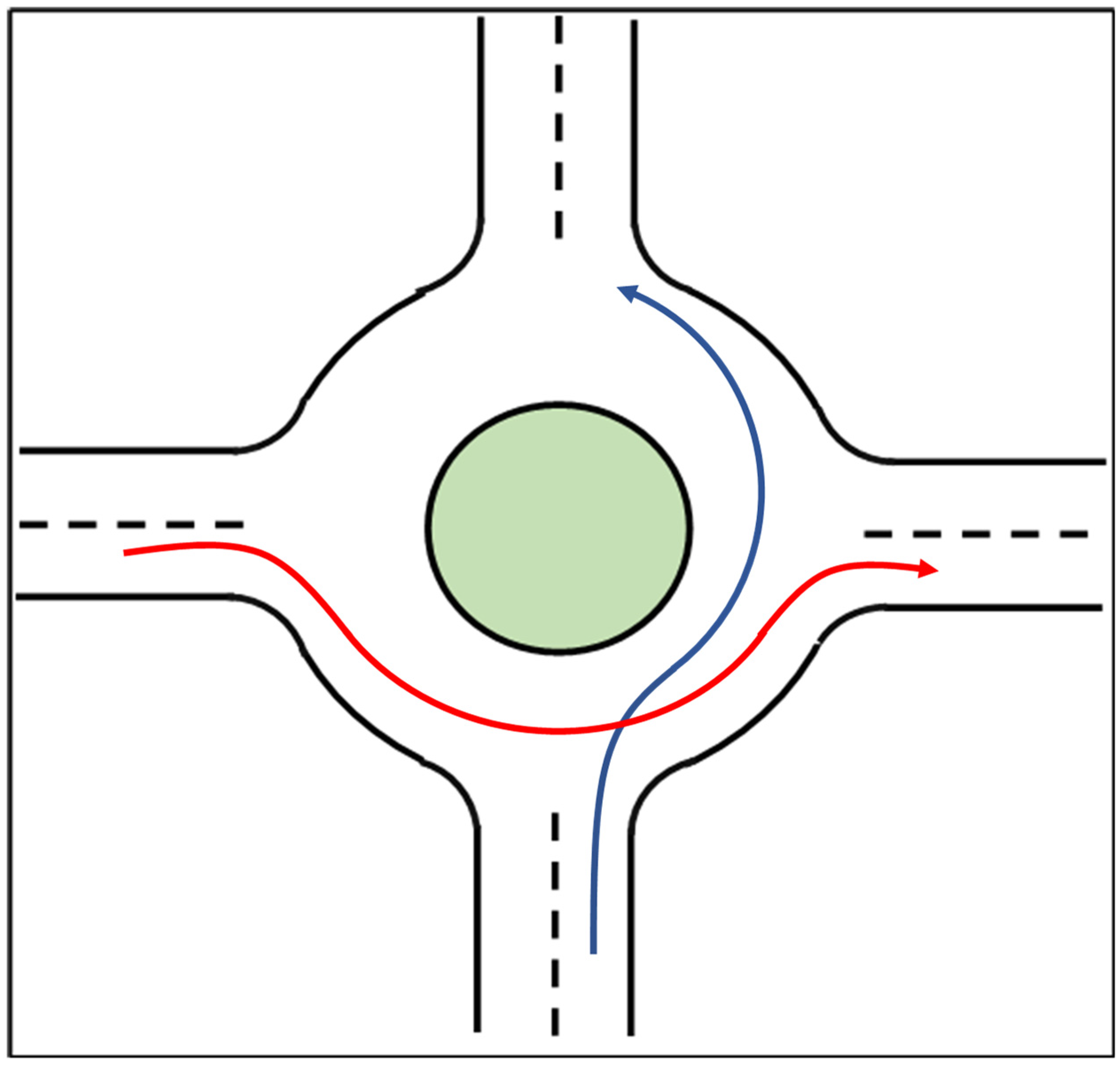
The goal of implementing the decision-making algorithm at a round intersection is to realize safe, comfortable and efficient driving of an autonomous vehicle that interacts with multiple other vehicles. To achieve this goal, not only is a decision-making algorithm necessary but good path planning is also required. However, path planning is out of the scope of this paper, and we will not discuss the path planning method here. The assumption made here is that the vehicle will drive on a designated path through a round intersection as illustrated in Figure 3 for two different vehicles. The blue line represents the path for the ego autonomous vehicle and the red line shows the path for another vehicle which could be a human driven vehicle or an autonomous vehicle. These two paths have an intersection point. Thus, to make sure that a collision does not happen at the intersection point between these two paths and that the ego-vehicle can pass through the round intersection within a shorter time as compared to executing a stop-wait-and-then-pass policy, a decision-making algorithm for a round intersection is necessary.

The vehicle model is an important factor for vehicle control in autonomous driving. Even though there is no perfect model to describe how the vehicle is moving, there are several vehicle models commonly used since they show good approximations and performance for the vehicle control problem. An example is the single-track vehicle model [11]. Autonomous vehicle control can be modeled in a hierarchical architecture. High level control for decision making and low level control for path following as well as the control for brake and throttle. In this paper, as we are mainly concentrating on the high-level decision making part of vehicle control, a model which describes the vehicle kinematic motion will be sufficient. Hence, we will be using the vehicle kinematic motion model in discrete time domain at a round intersection. The vehicle model for the ego vehicle with the subscript of r is given by

S_{t + 1} = T_{r} (S_{t}, a_{t})

(8)

where

S_{t}

represents the state vector of the vehicle and

a_{t}

is the input to drive the model. Model (8) is expanded in detail as,

x (t + 1) = x (t) + v (t) \cos θ (t) Δ t

(9)

y (t + 1) = y (t) + v (t) \sin θ (t) Δ t

(10)

v (t + 1) = v (t) + a (t) Δ t

(11)

θ (t + 1) = θ (t) + w (t) Δ t

(12)

In Equations (9)–(12),

x (t), y (t)

describe the 2D planar position and

θ (t)

is the heading angle of the vehicle model with respect to a fixed coordinate system.

v (t)

is the linear velocity of the vehicle. The input

a_{t}

that drives the vehicle is

〈 a (t), w (t) 〉

, the linear acceleration and the angular velocity or the yaw rate of the vehicle. The acceleration determines how fast the vehicle can change its speed and direction.

Δ t

is the time-step for the discrete model. In this paper, the above model is used for updating the states of the agent. Since the agent has no information of other vehicles, we assume that other vehicles will follow a similar model but with no speed or direction change given by

S_{t + 1} = T_{_{v}} (S_{t})

(13)

which can be expanded as

x (t + 1) = x (t) + v (t) \cos θ (t) Δ t

(14)

y (t + 1) = y (t) + v (t) \sin θ (t) Δ t

(15)

v (t + 1) = v (t)

(16)

θ (t + 1) = θ (t)

(17)

The position information, the heading angle and the velocity of other vehicles will be collected at each time a perception snapshot is made.

In this paper, the input of the ego vehicle is selected from a finite set of actions,

{a_{1}, a_{2}, ..., a_{m}} \times {w_{1}, w_{2}, ..., w_{k}}

for linear acceleration and angular velocity. At every decision step, the ego vehicle will take a linear acceleration for determining its velocity and an angular velocity for determining its direction of driving. The change of direction of the yaw rate introduces the discontinuity of tracking the vehicle motion using the model in Equation (8) and will influence the decision making for the forward Monte-Carlo simulation part and will be discussed in detail later.

In this paper, without loss of generality, all road users are considered as vehicles driving on the road. Based on the vehicle models provided, the state space of all the objects contains states of all the vehicles involved in the decision making problem. For the decision-making cycle at time

k

, the state space is given by

S_{k} = {s_{k}^{e}, s_{k}^{1}, ..., s_{k}^{m}}

(18)

The subscripts are the time stamps of the current decision-making cycle. The ego-vehicle’s state is represented with superscript

e

and superscripts

1, ..., m

are for the m other vehicles that are not controllable with the decision-making algorithm.

s^{e} = {[x, y, θ, v, w]}^{T}

x, y, θ

represent the longitudinal position, lateral position and yaw angle of the vehicle, respectively. These three values provide vehicle pose information.

v, w

are the linear velocity and yaw rate for describing the motion of the ego vehicle. For the other vehicles

s^{i} = {[x, y, θ, v]}^{T}, i = 1, ..., m

(19)

where

x, y, θ

are the vehicle pose information and

v

is linear velocity of the observed vehicle i. The difference in the state vector between the ego vehicle and other vehicles reveals the partial observability in vehicle decision making problems. Using the vehicle on-board sensors such as IMU, the ego vehicle can sense its yaw rate during driving. However, due to the limitation of sensors, the ego-vehicle will not be able to access other vehicles’ yaw rate values, hence the need to predict other vehicles’ future trajectories for planning and decision making. The transition models are the vehicle models provided before. We assume that the state transitions are deterministic with a probability of transition given by

T : P (s' | s, a) = 1

(20)

The observation states of the agent vehicle and the other vehicles are the same with their state vector with an observation probability of 1. The uncertainty of perception and sensing is not discussed here, and is out of the scope of this paper with

Z : P (o | s, a) = 1

(21)

Since the OOPOMDP method is employed for the decision-making problem with multi-vehicle round intersection traffic scenario, we also formalize the state space and observation space in the OOPOMDP fashion noting the following.

$C = {c_{r}, c_{v}}$ is the class of objects in the decision-making problem. In this problem, we consider two classes of objects which are the ego vehicle class $c_{r}$ for the ego vehicle and other vehicle class $c_{v}$ for other vehicles in the environment.
$A t t (C)$ are the attributes of objects in different classes. The attributes of the ego vehicle class include position information $(X, Y, θ)$ and motion information $(v, w)$ . The attributes of the other vehicle class include position information $(X, Y, θ)$ and velocity $v$ .
$D o m (a)$ is the domain of attributes. The domain of attributes in this paper is mainly on the poses of vehicles. For both the ego vehicle class and the other vehicle class, the positional domain is within the area of the round intersection, the heading angle is within the range of $[0, 2 π)$ .
A is action set. The action is a combination of two finite set of actions, $A = {a_{1}, a_{2}, ..., a_{m}} \times {w_{1}, w_{2}, ..., w_{k}}$ for linear acceleration and angular velocity. Each action is selected from the set and results in a pair $(a_{i}, w_{j}), i = 1... m, j = 1 \dots k$ .

The decision-making algorithm for a round intersection is based on the Partially Observable Markov Decision Making Process which can also be viewed as an optimization problem that optimizes the expected summary reward in the future horizon. Hence, a reward function or penalty function is required for awarding or penalizing the current action. In this paper, a penalty style reward function is implemented. Wrong actions will be penalized which makes it a negative reward. The goal of the decision-making algorithm is to minimize the overall negative reward (penalization) of the agent traveling along the designated path through the round intersection as given by

a^{*} = \underset{a \in A}{\arg \max} E [\sum_{t = 0}^{\infty} γ^{t} R (s_{t}, a_{t}) | b_{0}]

(22)

The goal of this decision-making algorithm is to make sure that the agent can drive through the round intersection safely, efficiently and comfortably. The requirements for these three perspectives lead to the penalization of the risk of collision, the speed, the acceleration, and the sound-use of the road. The overall reward function for each step is given by

R (s_{t}, a_{t}) = c_{1} R_{c o l l i s i o n} (s_{t}, a_{t}) + c_{2} R_{g a p} (s_{t}, a_{t}) + c_{3} R_{v e l o c i t y} (s_{t}, a_{t}) + c_{4} R_{t a r g e t} (s_{t}, a_{t}) + c_{5} R_{a c c} (s_{t}, a_{t})

(23)

The reward in Equation (23) is made up of five different components. For the collision reward, the ego vehicle should not collide with other road users as avoiding collisions and reducing traffic accidents is the top priority in designing any kind of decision-making algorithm. This reward is related to the nearest vehicle. Every time an action makes the ego vehicle get closer than some threshold safe distance to the nearest other vehicle, a large penalty given by

R_{c o l l i s i o n} (s_{t}, a_{t}) = {\begin{matrix} - 1000 if d (v_{e}, v) < = d_{s a f e} \\ 0 otherwise \end{matrix}

(24)

will be applied. In the above equation, d is the distance between the two vehicles given by

d (v_{e}, v) = \sqrt{| x_{e} - x |^{2} + | y_{e} - y |^{2}}

(25)

which is the distance between the center of mass of the agent vehicle (ego vehicle) and that of the nearest vehicle of detection.

d_{s a f e}

is determined by the dimensions of the vehicles and the speed limit of the road. As illustrated in Figure 4 below, for determining the safety bound of vehicles, a circular range around each vehicle is considered such that the boundary will not be influenced by the heading direction of vehicles. Therefore, the safety threshold distance is a summary of the threshold distance as well as the two radii of the circular boundaries generated from the vehicles’ dimensions and is given by

d_{s a f e} = d_{t h r e s h o l d} + R_{e, b o u n d a r y} + R_{b o u n d a r y}

(26)

d_{t h r e s h o l d} = \frac{v_{\lim}^{2}}{2 a_{\max}}

(27)

R_{e, b o u n d a r y} = \sqrt{W_{e}^{2} + {(L_{e} / 2)}^{2}}, R_{b o u n d a r y} = \sqrt{W^{2} + {(L / 2)}^{2}}

(28)

In Equations (26-28),

v_{\lim}

is the speed limit on a given road segment,

a_{m a x}

is the maximum allowed deceleration of a vehicle for which the passengers in the vehicle will not feel uncomfortable and

d_{t h r e s h o l d}

shows the emergency distance when the ego vehicle (the blue vehicle in the back) needs to make an emergency brake to fully stop in order to avoid collision with the front vehicle (the orange vehicle).

W

represents the width of the vehicles.

L

is the length of the vehicles.

The ego vehicle is penalized for its speed being lower than the speed limit of the current road segment as the vehicle is always expected to drive at the limit speed of the current road segment for efficiency. It is also penalized if it exceeds the speed limit. The penalty for exceeding the speed limit is larger than being lower than the limit speed. The penalty for discomfort is, then, introduced as

R_{v e l o c i t y} = {\begin{matrix} C_{e x c e e d} \frac{| v_{e} - v_{d e s} |}{v_{d e s}} if v_{e} > v_{d e s} \\ C_{l o w e r} \frac{| v_{e} - v_{d e s} |}{v_{d e s}} if v_{e} < v_{d e s} \end{matrix}

(29)

C_{e x c e e d}

and

C_{l o w e r}

are negative constant coefficients for the situation where ego velocity

v_{e}

is larger than or smaller than the desired velocity

v_{d e s}

, respectively. The desired velocity is determined according to the largest tolerance to lateral acceleration for passengers in the vehicle if the vehicle is turning and follows the road speed limitation if the vehicle is traveling on straight road as

v_{d e s} = {\begin{matrix} \sqrt{a_{y, \max} / κ} if turning \\ v_{l i m i t} otherwise \end{matrix}

(30)

κ

in Equation (30) is the radius of curvature while turning. The velocity reward will drive the ego vehicle towards desired velocity if there is no risk of collision with the other vehicles. If there is a chance of collision, the velocity reward will be dominated by the penalty caused by collision risk due to the difference of scales between these two rewards. Regarding the comfort of the passengers in the vehicle, the maximum acceleration is limited as

a = \sqrt{a_{x}^{2} + a_{y}^{2}} < = a_{\max} .

(31)

Therefore, once the overall acceleration is larger than

a_{\max}

, a penalty for discomfort is introduced in the reward function for causing discomfort to the passengers in the vehicle. The longitudinal acceleration part

a_{x}

is the currently selected action from the action set. The lateral acceleration

a_{y}

is derived from the lateral motion of the vehicle as

a_{y} = v^{2} / r = v^{2} κ

(32)

Since the vehicle is following a designated path, the target area is also pre-determined on the path. Once the vehicle is within the target point of the path, it will be rewarded.

Apart from the commonly seen reward settings as can be seen in other works, a gap reward is also proposed for driving efficiency on the road in the decision-making algorithm of this paper. Intersections, especially round ones, are the most crowded traffic scenarios in urban traffic with vehicles merging from different road segments. Besides the requirement of safety, efficient use of the road space is also necessary to reduce the chance of traffic jam. The gap reward aims to drive the agent vehicles to follow the proceeding vehicle at a certain distance. A commonly accepted 3-second rule for vehicle following is adopted for generating the desired gap between the agent vehicle with the preceding vehicle as

v_{3 s} = \max {v_{e} - 3 * b_{\max}, 0}

(33)

d_{d e s i r e d} = \frac{v_{e}^{2} - v_{3 s}^{2}}{2 a_{\max}}

(34)

R_{g a p} = c_{g a p} | d (v_{e}, v) - d_{d e s i r e d} |

(35)

Here in Equation (33),

v_{3 s}

is the target velocity when acting emergency full brake at the maximum brake acceleration

b_{\max}

and

d_{d e s i r e d}

is the preferred gap between the ego vehicle and the nearest preceding vehicle. A negative reward R_gap will be assigned according to Equation (35) if the distance is different from the desired gap between vehicles.

3. Improving Decision Making with Policy Prediction

Decision making and planning for autonomous vehicles in urban traffic scenarios has always been a challenging problem due to the complexity of urban traffic. Another challenge is the tracking of vehicle driving motion in the urban area that largely influences the performance of the decision-making algorithm. There are several research works that have been conducted to improve the vehicle planning algorithm performance. Reference [21] proposes the method of adjusting the vehicle model parameters (Intelligent Driver Model or IDM model parameters) to emulate different style of driving and tries to improve the decision-making algorithm for highway autonomous driving performance. Reference [22] proposed a game-theoretic planning algorithm for all vehicles in the traffic scenario in round intersections. Reference [23] proposed a method that uses hidden mode stochastic hybrid system to model different human driving behaviors to assist the performance of decision making in a driver assistance system. Yet, there are rare works for improving the autonomous vehicle decision making problem for round intersections with multiple vehicles involved. Hence, in this section, a policy prediction method based improvement for autonomous vehicle decision making is proposed as one of the main contributions of this paper.

The planning and decision-making problem can be regarded as a receding horizon optimization problem starting from current time and extending to a future time based on the horizon of the optimization problem. The ego vehicle obtains an observation of all the other surrounding vehicles at time t, noted as

o_{t}

and tries to find an optimal action such that the total reward is maximized as

a^{*} = \underset{a \in A}{\arg \max} E [\sum_{t = t}^{t + k} γ^{t} R (s_{t}, a_{t})] .

(36)

We do not have full knowledge of all the future states along the planning horizon. It is essential to have a good prediction over the future state trajectories and the state transition model needs to have good precision on tracking the future potential trajectories.

For decision making and planning of autonomous vehicles, the vehicle trajectory tracking over a future horizon can be done with the state transition model as described in Equations (13) – (17). For highways, it is rather simple since the vehicles tend to not have rough behaviors like multiple lane-changing within a short time for example. The model in Equation (13) can provide good trajectory tracking for the decision-making problem on a highway. The case is different for planning in the urban traffic environment for intersections, especially round intersections. The vehicle needs to change the direction of driving in a short period of time due to the geometric features of intersections. The current observations of other vehicles do not provide enough information on how they will be moving in the future time horizon for planning.

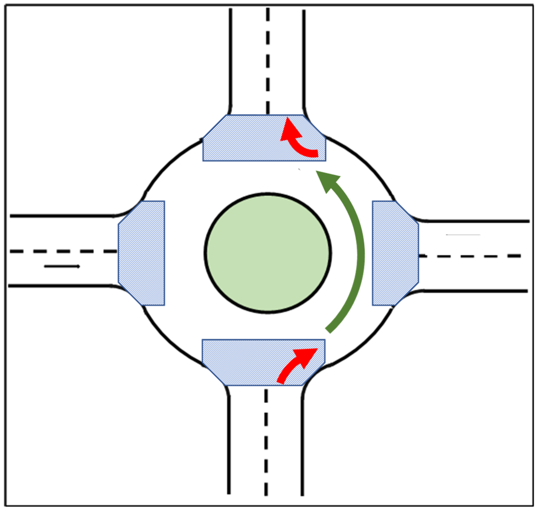
As a demonstration example, the path of a vehicle passing a round intersection is shown in Figure 5. The shadowed areas in the figure are the areas in which a vehicle is entering or exiting the round intersection. The vehicle first travels through a shadowed area to enter the round intersection and takes a turn in clockwise direction as shown by the bottom red arrow. After passing the shadowed area to enter the round intersection, the vehicle follows the lane area and takes a constant yaw angle turning in the counterclockwise direction as shown by the green arrow. Reaching the target connection point to exit, the vehicle now, takes a clockwise turn to exit the round intersection and drive on the straight road again as shown by the red arrow on the top. Through the whole procedure of passing the round intersection, the vehicle shows a discontinuous motion in driving direction and the yaw rate keeps changing along the path and makes it hard for the vehicle motion model (10) to track given a single initial condition.

In a decision making cycle, the planning starts from some initial state sampled from the belief state space at current time, denoted as

t_{0}

, and carries out a forward simulation to generate potential trajectories of the states for optimizing the expected cumulative reward along the optimization horizon

t_{0} ~ t_{0} + k

, with

k

being the decision making horizon. Directly implementing the vehicle motion models in Equation (10), even with the knowledge of yaw rate at

t_{0}

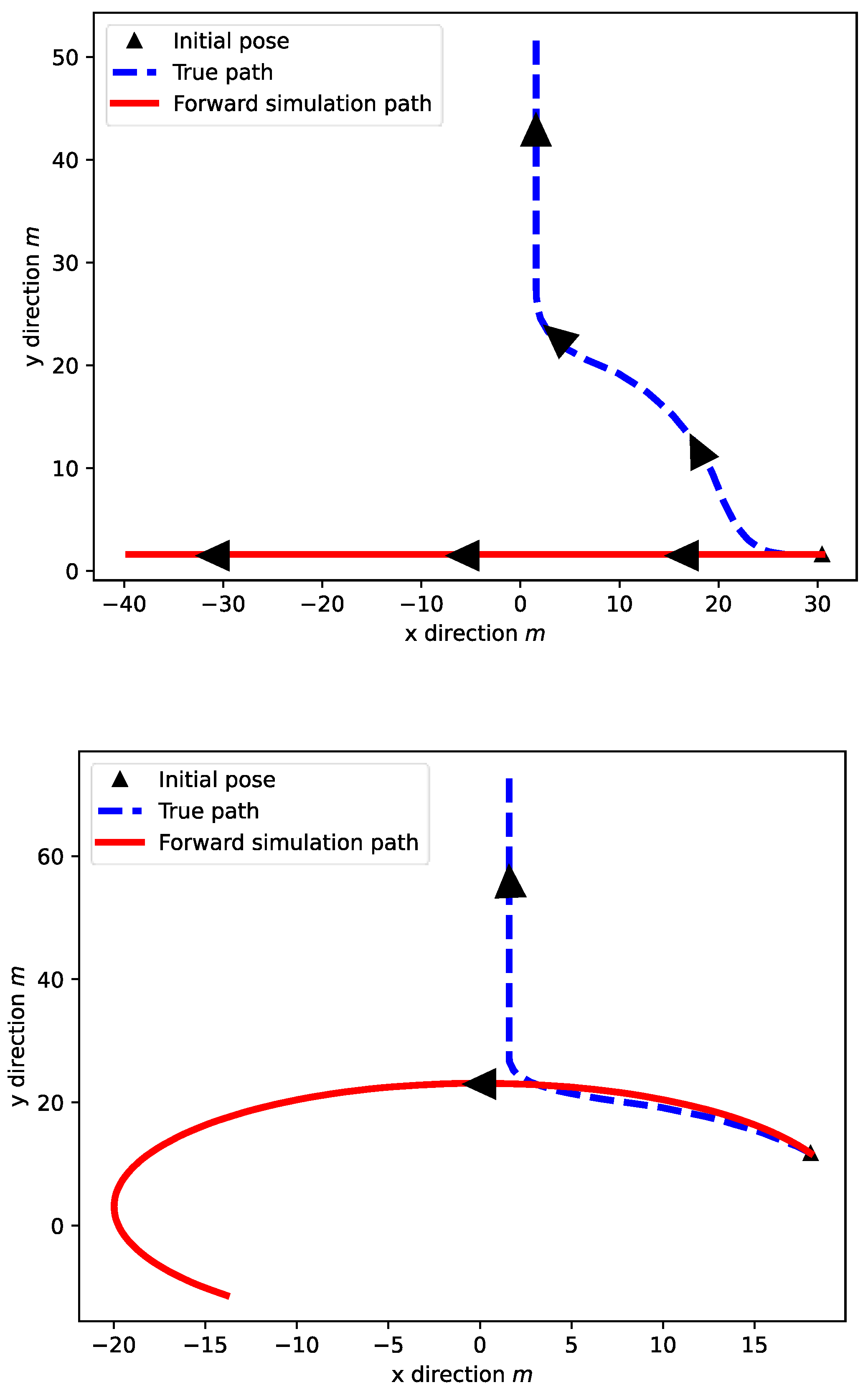
, the true trajectory deviates a lot from the simulated trajectory that tracks the potential vehicle trajectory on the optimization horizon. The model alone is not enough to describe the vehicle state transitions under the round intersection traffic scenarios, as shown in Figure 6. In Figure 6, the true trajectories are not successfully tracked by directly implementing the state transition equations from the initial state. The forward simulation path is calculated for 100 steps and the arrows show the direction of the vehicle moving or the direction of simulation. This will cause a lot of issues when making decisions for the ego vehicle to pass the round intersection safely and efficiently. This issue will also affect the solution of the POMDP problem based on Monte-Carlo Tree search since Monte- Carlo simulation for the state particles is the core procedure for the tree search algorithm.

To overcome the issue caused by discontinuity of vehicle motion, a policy prediction based decision making method is proposed here such that the state transition of the vehicle can be better tracked and simulated during the decision making cycle. The policy prediction method is based on change point policy prediction method. This paper mainly focuses on the traffic scenario of round intersections and an abstract policy set is applied here for the decision making algorithm. This method utilizes the recorded history of the decision-making algorithm based on OOPOMDP so that it avoids additional memory cost.

4. Augmented Objective State and Policy Based State Transition

The original setting of the observation state is the same as the state of other vehicles, that is

s_{t}^{i} = o_{t}^{i} = {[x_{i}, y_{i}, θ_{i}, v_{i}]}^{T}

(37)

where, the observation state

o_{t}^{i}

is the real observation made by the agent from the environment. It does not contain any of the policy information so that the states sampled from the updated belief states will directly accomplish state transition using the model (10) during the decision cycle. This will lead to the issue of the simulated path deviating from the true path and causing inaccuracy of decision making. Here, an attribute is added to other vehicle class

c_{v}

for the most recent policy

π_{i}

that augments the state space and observation space into

s_{t, a}^{i} = o_{t, a}^{i} = {[x_{i}, y_{i}, θ_{i}, v_{i}, π_{i}]}^{T}

(38)

where

π_{i}

is the most likely policy that the observed vehicle is executing at the time that current observation is made for vehicle i. Denote the policy prediction method as

F : h \to π_{t}^{i}, i \in {1, 2, ..., n}

(39)

Here,

h

is the current history in the POMDP problem, and as shown in a previous section, is a series of actions and observations made by the agent and given by

h_{t} = {b_{0}, a_{0}, o_{1}, a_{1}, o_{2}, ..., a_{t - 1}, o_{t}} .

(40)

According to the feature of OOPOMDP, the observations of other vehicles can also be indexed by object in the history. So, we can use it for policy prediction method for each of the vehicles involved in the traffic scenario.

π_{t}^{i} \in Π

is a policy for vehicle i selected from the pre-determined policy set. For every decision cycle, we first obtain the history of observations on vehicle

i

and implement the policy prediction method to find the policy over the last segment of the vehicle, then augment the observations state and state of vehicle i with the potential policy so that the policy can be used for state transition during the Monte-Carlo Tree search. The state transition equation of other vehicles is now modeled as

S_{t + 1} = T_{v} (S_{t}, π_{t})

(41)

with

x (t + 1) = x (t) + v (t) \cos θ (t) Δ t

(42)

y (t + 1) = y (t) + v (t) \sin θ (t) Δ t

(43)

v (t + 1) = v (t)

(44)

θ (t + 1) = θ (t) + w (π_{i}, {\hat{θ}}_{π_{i}}) d t

(45)

The vehicle model (13) now becomes a constant velocity and turn rate model for vehicle trajectory tracking. The yaw rate is generated based on current policy

π_{i}

and parameter

{\hat{θ}}_{π_{i}}

that will help with the vehicle trajectory tracking in the decision-making cycle and improve the performance of the decision making based on the OOPOMCP algorithm.

Since the decision-making algorithm is mainly used for vehicles traversing the round intersection, we take advantage of its geometry to simplify the generation procedure of vehicle yaw rate based on the policy. According to the geometric features of the round intersection, we know that a round intersection has mainly three types of areas: straight road segments, enter/exit area and round area. The vehicle yaw rate will also be determined by the road curvatures in these three different types of areas based on

w = v / r = v \cdot κ

(46)

where r is the turning radius of the vehicle trajectory and

κ

is the road curvature.

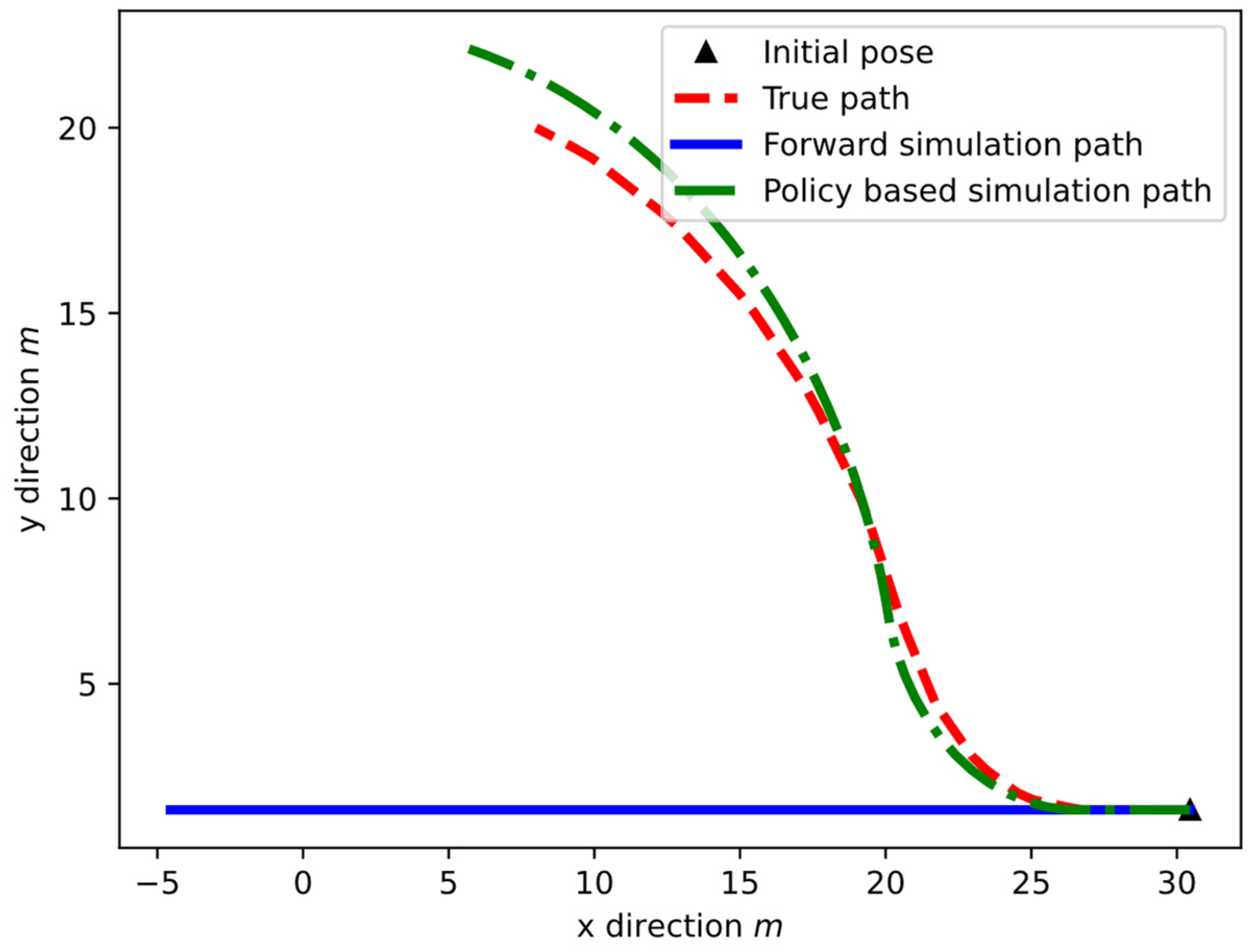
To illustrate the difference in utilizing this method, a forward simulation trajectory is generated by the policy-based state transition model and shown Figure 7. From Figure 7, we can see that the policy based simulated path is very similar to the true path of a vehicle passing the round intersection where only the initial state is given. In the simulated path generation, we assume that the policy of entering the round intersection is given such that the vehicle yaw rate is generated based on the policy, so the vehicle is turning in a clockwise direction to enter the round intersection instead of keeping the original heading angles and yaw rate from the straight lane. In this case, the decision made by the agent vehicle will be closer to the real situation and improve the performance of the decision-making algorithm.

Besides using the policy-based state transition in the decision making problem of vehicles in a round intersection, the control of the autonomous vehicle also considers vehicle jerk. Since the reward function can measure how good it is for current selection of an action from the action set, it is able to measure the rewards caused by velocity that exceeds the speed limit or exceeds the maximum lateral acceleration that causes discomfort. However, it is not capable of measuring the change of acceleration (jerk) since the reward function does not have access to previous actions. Therefore, the previous linear acceleration is stored for comparison with current acceleration determined by the tree search. We approximate the jerk of the vehicle to be given by

J_{t} = | Δ a | = | a_{t} - a_{t - 1} |

(47)

Based on this jerk indication

J_{t}

, an acceleration re-selection is made to ascertain that the acceleration change does not exceed a maximum allowed jerk so that the vehicle speed change is smooth and passengers will feel comfortable. This is based on

a_{t} = {\begin{matrix} a_{t} if J_{t} < = J_{\max} \\ \begin{matrix} a_{t - 1} + J_{m a x} if a_{t} - a_{t - 1} > = J_{\max} \\ a_{t - 1} - J_{m a x} if a_{t} - a_{t - 1} < = - J_{\max} \end{matrix} \end{matrix}

(48)

which is used to make sure that the jerk of the autonomous vehicle will not be too large.

5. Simulations and Discussion

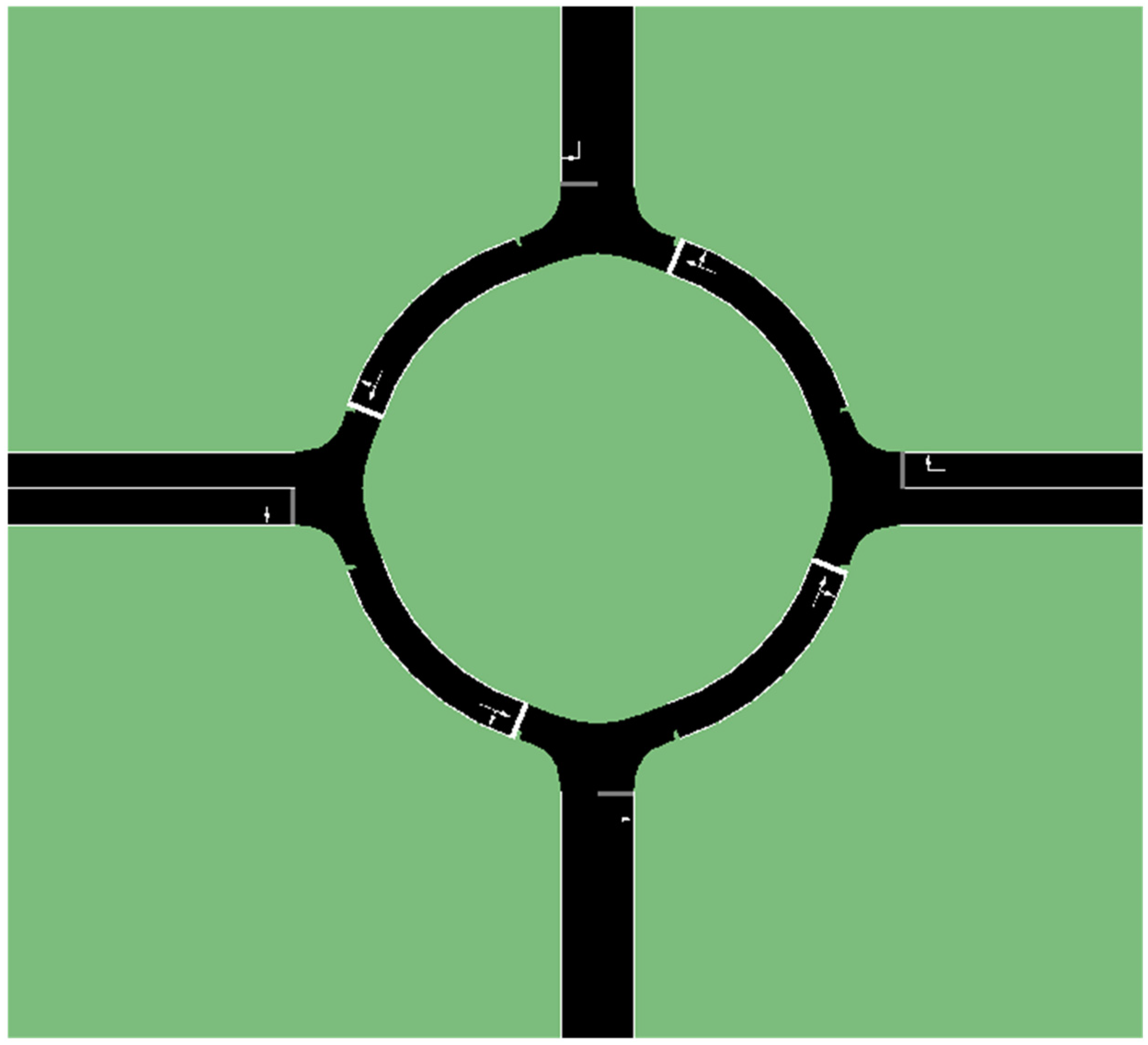
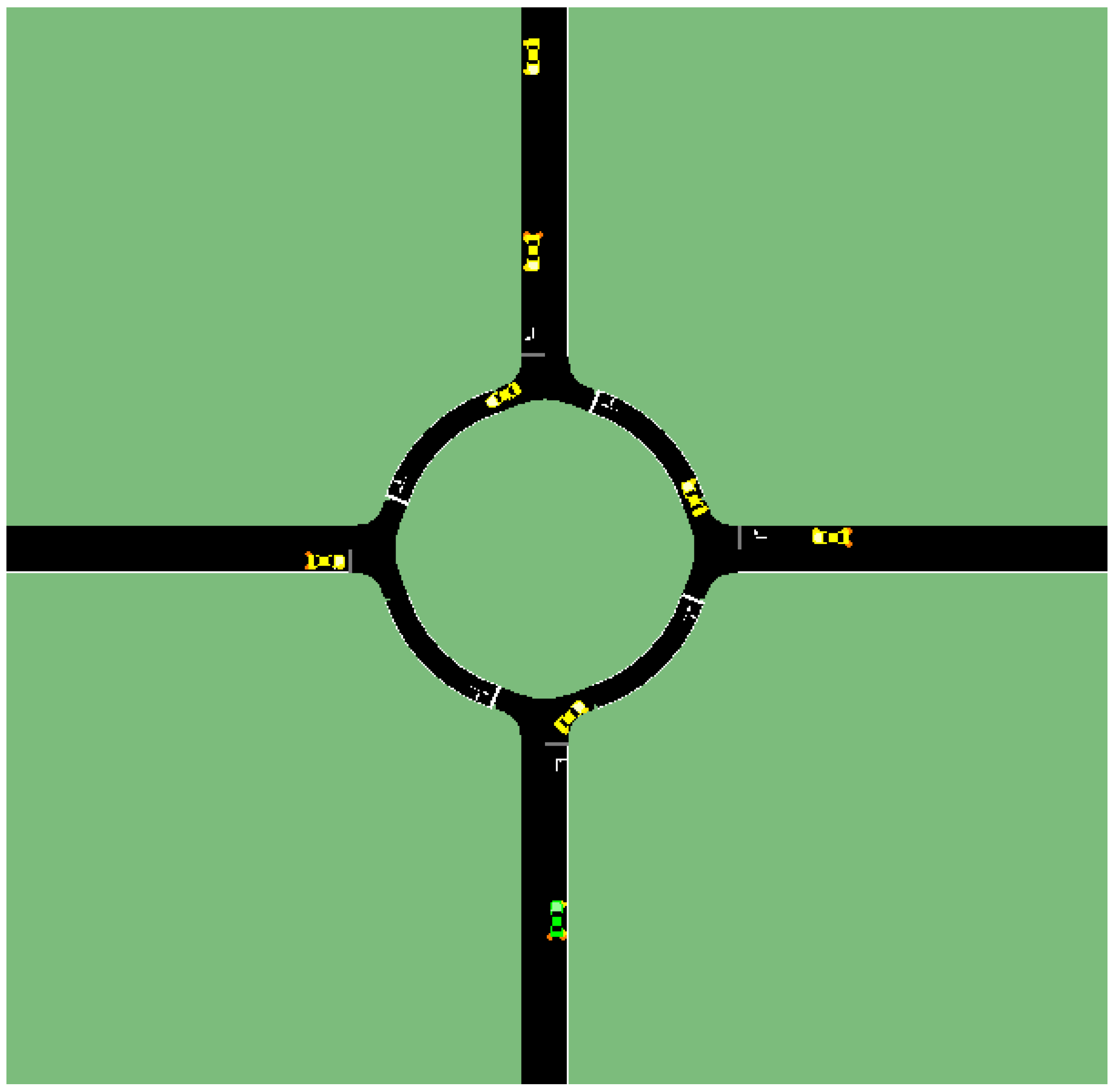
The simulation of decision making for autonomous vehicles passing a round intersection is carried out and exemplary results are summarized here to test and validate the decision making algorithm with policy based state transition. The traffic scenario in the simulation is a typical 4-way round intersection as shown in Figure 8. Vehicles enter the scenario from the straight lane segment and move towards its destination area. For simplifying the test environment, we assume the round intersection is a circle so that the road curvature within the round intersection is a constant:

κ = 1 / r

where

r

is the radius of curvature of the lanes in the round intersection. During the simulation, vehicles drive on the right side of the road on the straight lane segment and in the counterclockwise direction while they are within the round intersection.

For the OOPOMCP algorithm to solve the Object-Oriented POMDP Problem, the parameters used in the tree search are:

Planning time for each step: 1.0 s
Maximum search depth in the tree: 100
Exploration constant value: 2.0
Discount factor of the cumulative expected reward: 0.99

In the action set, the discrete linear acceleration set given by

A c c = {- 3.0, - 2.0, - 1.0, 0, 0.5, 1.5, 2.5} m / s^{2}

(49)

is used. The yaw rate of the vehicle can be determined according to the road curvature using the linear velocity at different road segments for the round intersection. As for a single lane round intersection with straight road segment connecting to it, the yaw rate appears to have 3 features:

In the straight lane segments, the vehicle’s yaw rate is maintained at zero as it keeps driving straight.
In the round intersection part, the vehicle will drive along the road at the yaw rate of $w = \frac{v}{R}$ where $R$ is the radius of the round intersection and $v$ is the vehicle linear velocity, and this is a positive value when setting the counterclockwise direction as the positive direction.
When the vehicle is entering/exiting the round intersection, the yaw rate $w'$ , is some negative value when the counterclockwise direction is taken as the positive direction. In the simulation, since the entering/exiting process only takes a very short time of period, the yaw angle change is approximated with a yaw rate determined by the process of uncontrolled simulation vehicles entering the round intersection.

In the simulation, the round intersection has a radius of curvature of 20 m, hence the road curvature in the roundabout intersection is 1/20. Additionally, based on the test data, the curvature of the entering/exiting area in the simulation is approximated to be 0.15 and will be used in the transition model. Apart from those parameters in the action set, parameters for the reward function in the decision-making problem are listed below. Currently, all the factors in the total reward are equally weighted, hence the coefficients used are

c_{1} = c_{2} = c_{3} = c_{4} = c_{5} = 1 .

(50)

The collision reward depends on the vehicle dimensions. In this test, the vehicles have same dimension, which are

L = 5.0 m, W = 1.8 m

, which is the default settings of the passenger vehicles in SUMO simulation.

The overall maximum acceleration required in Equation (14) is set to be 4.0

m / s^{2}

, and the maximum lateral acceleration caused by vehicle turning is set to be 2.0

m / s^{2}

. The cost due to exceeding the desired velocity in Equation (10) is

C_{e x c e e d} = - 100

for penalizing the unsafe maneuvering of exceeding the maximum allowed velocity, and the cost for being lower than the desired velocity is

C_{l o w e r} = - 10

. The maximum brake acceleration is the lowest acceleration from the action set that is -3.0

m / s^{2}

and

c_{g a p} = - 10

．

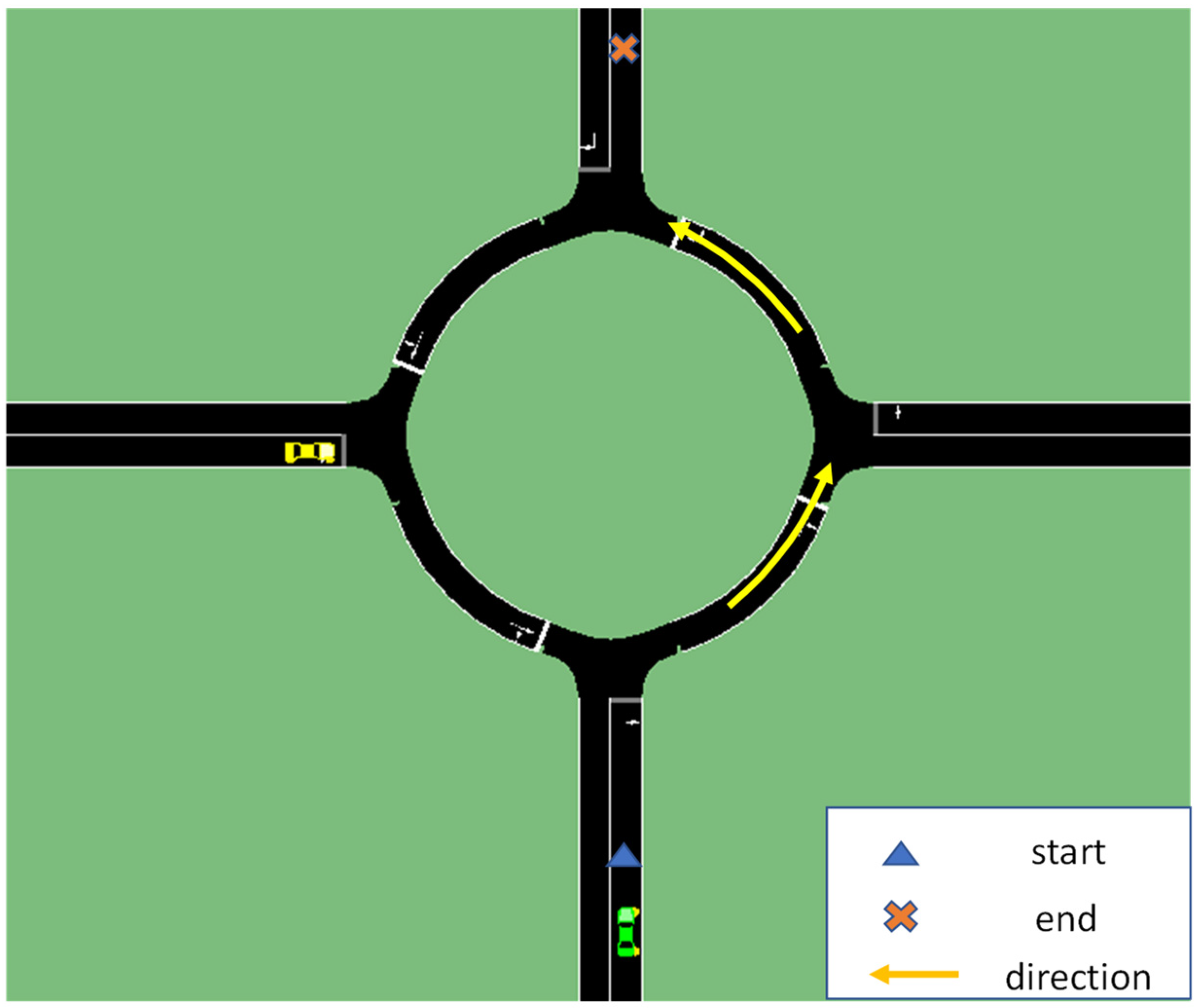
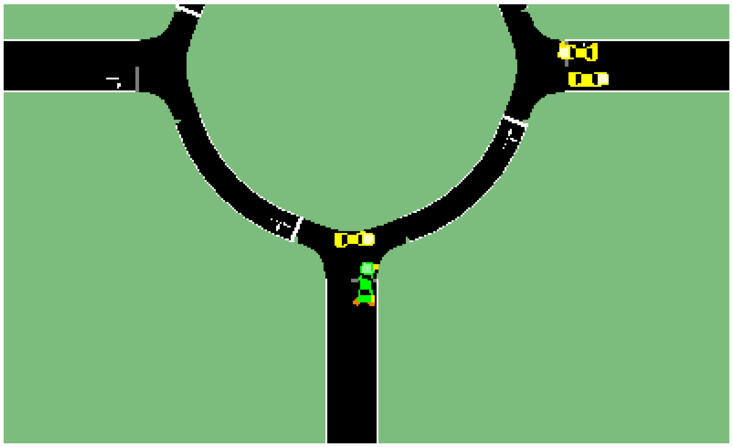
The simulation results compare the performance of the decision-making algorithm with decision making using OOPOMDP with and without policy-based state transition against the benchmarking system of the SUMO simulation system built in vehicle model, which is an Intelligent Driver Model (IDM) that executes lane following. The results compare the total travel time, total reward and if there is emergency brake acted by other vehicles in the system. First a two-vehicle scenario simulation is done, and the results are presented below. The diagram of the two-vehicle scenario is presented in Figure 9. The autonomous vehicle colored green is traversing the round intersection starting from the bottom and trying to reach the destination points at the top in the figure. The simulation results for this two-vehicle scenario are summarized in Table 1.

From the results above in Table 1, we can find that the OOPOMDP with policy based state transition method proposed in this paper achieves higher reward (less negative) compared with the one which directly implements the state transition model proposed in Equation (13). With the policy-based state transition, the ego vehicle can better predict the future trajectory of the surrounding vehicles and control the speed and direction to reach destination in a shorter time. Also, since it avoids the risk of colliding with other vehicles, no emergency brake or aggressive maneuvers need to be made by other vehicles while they are following the lane with their IDM models. Also, the shorter time achieved when comparing to the system driver proves the efficiency of implementing such decision-making algorithm for autonomous vehicles in round intersections.

Another simulation is carried out for a multi-vehicle scenario. Eight vehicles in total are involved in the simulation with different departure times. Hence, they will interact within the region of the round intersection, as shown in Figure 10. The green vehicle shows the ego vehicle that deploys the decision-making algorithm, and the test results are summarized in Table 2.

In this simulation whose results are summarized in Table 2, the decision making with policy-based state transition is able to achieve the goal of traversing the round intersection safely and efficiently without any potential collision and takes advantage of road space to drive fast. Yet, we see that the OOPOMDP based decision making has large penalty (negative total reward) because a potential collision that generates a very large penalty happens due to the inaccuracy of predicting other vehicles’ trajectories as shown in Figure 11. The long traversal time of the system driver is due to the right of way. The ego vehicle has to wait for other vehicles to pass in the round intersection. Thus, the waiting time is very long as compared to the result of implementing the POMDP decision making algorithms of this paper.

6. Conclusions and Recommendations

In this paper, methods for decision making and planning of autonomous vehicles in handling a round intersection were introduced and discussed along with simulation results for validation of the algorithms. POMDP was first introduced as a powerful tool for solving the sequential decision-making problem with uncertainties and states that are not fully observable. The OOPOMDP algorithm was later introduced as a method for factoring object states and observations individually and making the belief update more efficient and low cost. Utilizing the feature of OOPOMDP, a policy-based state transition was employed for the decision-making algorithm. Since the OOPOMDP stores the history of all the involved agents and environment objects, the agent gets to determine the most recent policy of other vehicles based on the policy prediction method that was introduced. This OOPOMDP decision-making with policy prediction largely improves the performance of the decision making for the traffic scenario of round intersections. The reward function was formulated for safe and efficient travel while keeping passenger comfort in mind.

The approach in this paper can be applied to other relevant connected and autonomous driving tasks. For example, platooning or convoying of vehicles in the form of adaptive and cooperative adaptive cruise control [24,25] on highways is a topic of high research attention. More recent work focuses on similar cooperative driving in urban roads including cooperative handling of an intersection by a convoy of cooperating vehicles [26]. While there are results for straight intersections, corresponding results for round intersections are missing. The approach in this paper can be useful for cooperative handling of round intersections by a convoy of connected and autonomous vehicles. Active safety control systems like yaw stability controllers [27,28] are also important as the vehicles in the round intersections follow a circular path and yaw stability problems may occur due to weather conditions or emergency maneuvers. Extension of the approach of this paper can incorporate a more detailed model of the ego vehicle and can be integrated with yaw stability control to accommodate such problems.

Author Contributions

Conceptualization, X.L., L.G. and B.A.-G.; methodology, X.L. and L.G.; software, X.L.; validation, X.L.; formal analysis, X.L.; investigation, X.L.; resources, L.G. and B.A.-G.; data curation, X.L.; writing—original draft preparation, X.L.; writing—review and editing, L.G. and B.A.-G.; visualization, X.L.; supervision, L.G.; project administration, L.G. and B.A.-G..; funding acquisition, L.G. and B.A.-G. All authors have read and agreed to the published version of the manuscript.

Funding

The authors acknowledge the partial support through the Smart Campus organization (21824) of the Ohio State University in support of the Smart Columbus project.

Data Availability Statement

Not applicable.

Acknowledgments

The authors thank the support of the Automated Driving Lab at the Ohio State University.

Conflicts of Interest

The authors declare no conflict of interest.

References

Gkartzonikas, C.; Gkritza, K. What have we learned? A review of stated preference and choice studies on autonomous vehicles. Transp. Res. Part C: Emerg. Technol. 2018, 98, 323–337. [Google Scholar] [CrossRef]
Rana, M.; Hossain, K. Connected and Autonomous Vehicles and Infrastructures: A Literature Review. Int. J. Pavement Res. Technol. 2021, 16, 264–284. [Google Scholar] [CrossRef]
Reyes-Muñoz, A.; Guerrero-Ibáñez, J. Vulnerable Road Users and Connected Autonomous Vehicles Interaction: A Survey. Sensors 2022, 22, 4614. [Google Scholar] [CrossRef]
Sadid, H.; Antoniou, C. Modelling and simulation of (connected) autonomous vehicles longitudinal driving behavior: A state-of-the-art. IET Intelligent Transport Systems 2023, 17, 1051–1071. [Google Scholar] [CrossRef]
Guvenc, L.; Guvenc, B.A.; Emirler, M.T. Connected and Autonomous Vehicles. In Internet of Things and Data Analytics Handbook; John Wiley & Sons, Ltd.: Hoboken, NJ, USA, 2017; ISBN 978-1-119-17360-1. [Google Scholar]
Claussmann, L.; Revilloud, M.; Gruyer, D.; Glaser, S. A Review of Motion Planning for Highway Autonomous Driving. IEEE Trans. Intell. Transp. Syst. 2019, 21, 1826–1848. [Google Scholar] [CrossRef]
Kuwata, Y.; Teo, J.; Fiore, G.; Karaman, S.; Frazzoli, E.; How, J.P. Real-Time Motion Planning With Applications to Autonomous Urban Driving. IEEE Trans. Control Syst. Technol. 2009, 17, 1105–1118. [Google Scholar] [CrossRef]
Yurtsever, E.; Lambert, J.; Carballo, A.; Takeda, K. A Survey of Autonomous Driving: Common Practices and Emerging Technologies. IEEE Access 2020, 8, 58443–58469. [Google Scholar] [CrossRef]
Kuutti, S.; Fallah, S.; Katsaros, K.; Dianati, M.; Mccullough, F.; Mouzakitis, A. A Survey of the State-of-the-Art Localization Techniques and Their Potentials for Autonomous Vehicle Applications. IEEE Internet Things J. 2018, 5, 829–846. [Google Scholar] [CrossRef]
Guvenç, L.; Guvenç, B.A.; Demirel, B.; Emirler, M.T. Control of Mechatronic Systems; IET Control, Robotics and Sensors Series, Ed.; The Institute of Engineering and Technology: London, UK, 2017; ISBN 978-1-78561-145-2. [Google Scholar]
Güvenç, L.; Aksun--Güvenç, B.; Zhu, S. ; Gelbal,.Y. Autonomous Road Vehicle Path Planning and Tracking Control; Wiley: Hoboken, NJ, United States, 2021; ISBN 9781119747949. [Google Scholar]
Li, S.; Shu, K.; Chen, C.; Cao, D. Planning and Decision-making for Connected Autonomous Vehicles at Road Intersections: A Review. Chin. J. Mech. Eng. 2021, 34, 1–18. [Google Scholar] [CrossRef]
Schwarting, W.; Alonso-Mora, J.; Rus, D. Planning and Decision-Making for Autonomous Vehicles. Annu. Rev. Control. Robot. Auton. Syst. 2018, 1, 187–210. [Google Scholar] [CrossRef]
Al-Turki, M.; Ratrout, N.T.; Rahman, S.M.; Assi, K.J. Signalized Intersection Control in Mixed Autonomous and Regular Vehicles Traffic Environment—A Critical Review Focusing on Future Control. IEEE Access 2022, 10, 16942–16951. [Google Scholar] [CrossRef]
Li, X.; Doss, A.C.A.; Guvenc, B.A.; Guvenc, L. Pre-Deployment Testing of Low Speed, Urban Road Autonomous Driving in a Simulated Environment. SAE Int. J. Adv. Curr. Pr. Mobil. 2020, 2, 3301–3311. [Google Scholar] [CrossRef]
Li, X.; Zhu, S.; Aksun-Guvenc, B.; Guvenc, L. Development and Evaluation of Path and Speed Profile Planning and Tracking Control for an Autonomous Shuttle Using a Realistic, Virtual Simulation Environment. J. Intell. Robot. Syst. 2021, 101, 1–23. [Google Scholar] [CrossRef]
Ye, N.; Somani, A.; Hsu, D.; Lee, W.S. DESPOT: Online POMDP Planning with Regularization. J. Artif. Intell. Res. 2017, 58, 231–266. [Google Scholar] [CrossRef]
Wandzel, A.; Oh, Y.; Fishman, M.; Kumar, N.; Wong, L.S.; Tellex, S. Multi-object search using object-oriented POMDPs. In Proceedings 2019 International Conference on Robotics and Automation (ICRA) 2019, 7194-7200. IEEE.
Silver, D.; Veness, J. Monte-Carlo planning in large POMDPs. In Proceedings Advances in neural information processing systems 2010, 2164–2172. [Google Scholar]
Hubmann, C.; Schulz, J.; Becker, M.; Althoff, D.; Stiller, C. Automated Driving in Uncertain Environments: Planning With Interaction and Uncertain Maneuver Prediction. IEEE Trans. Intell. Veh. 2018, 3, 5–17. [Google Scholar] [CrossRef]
Sriram, N. , Liu, B., Pittaluga, F., Chandraker, M.: Smart: Simultaneous multi-agent recurrent trajectory prediction. In: European Conference on Computer Vision 2020, pp. 463-479.
Tian, R.; Li, S.; Li, N.; Kolmanovsky, I.; Girard, A.; Yildiz, Y. Adaptive Game-Theoretic Decision Making for Autonomous Vehicle Control at Roundabouts. 2018 IEEE Conference on Decision and Control (CDC). LOCATION OF CONFERENCE, COUNTRYDATE OF CONFERENCE; pp. 321–326.
Lam, C.-P.; Yang, A.Y.; Driggs-Campbell, K.; Bajcsy, R.; Sastry, S.S. Improving human-in-the-loop decision making in multi-mode driver assistance systems using hidden mode stochastic hybrid systems. 2015 IEEE/RSJ International Conference on Intelligent Robots and Systems (IROS). LOCATION OF CONFERENCE, GermanyDATE OF CONFERENCE;
Emirler, M.T.; Güvenç, L.; Güvenç, B.A. Design and Evaluation of Robust Cooperative Adaptive Cruise Control Systems in Parameter Space. Int. J. Automot. Technol. 2018, 19, 359–367. [Google Scholar] [CrossRef]
Ma, F.; Wang, J.; Zhu, S.; Gelbal, S.Y.; Yang, Y.; Aksun-Guvenc, B.; Guvenc, L. Distributed Control of Cooperative Vehicular Platoon With Nonideal Communication Condition. IEEE Trans. Veh. Technol. 2020, 69, 8207–8220. [Google Scholar] [CrossRef]
Ma, F.; Yang, Y.; Wang, J.; Li, X.; Wu, G.; Zhao, Y.; Wu, L.; Aksun-Guvenc, B.; Guvenc, L. Eco-driving-based cooperative adaptive cruise control of connected vehicles platoon at signalized intersections. Transp. Res. Part D: Transp. Environ. 2021, 92. [Google Scholar] [CrossRef]
Guvenc, B.; Guvenc, L.; Ozturk, E.; Yigit, T. Model regulator based individual wheel braking control. Conference on Control Applications. LOCATION OF CONFERENCE, TurkeyDATE OF CONFERENCE; pp. 31–36.
Aksun-Guvenc, B.; Guvenc, L. The Limited Integrator Model Regulator and its Use in Vehicle Steering Control. Turkish Journal of Engineering and Environmental Sciences 2002, 473–482. [Google Scholar]

Figure 1. Diagram of a round intersection with arrows showing allowed direction of travel.

Figure 2. Diagram of sequential decision-making problem.

Figure 3. Diagram of two vehicles passing through the round intersection.

Figure 4. Diagram of reward (cost) for collision.

Figure 5. Diagram of vehicle passing a round intersection (vehicles enter/exit the round intersection through the shaded areas, arrows show direction of travel).

Figure 6. Forward simulated path obtained by using the state transition model directly, large arrows show direction of travel.

Figure 7. Policy based forward simulation.

Figure 8. SUMO simulation environment.

Figure 9. Two-vehicle scenario of passing the intersection.

Figure 10. Multi-vehicle scenario.

Figure 11. Potential collision.

Table 1. Simulation Result of the 2-vehicle Scenario.

	Total Reward	Total Travel time	Emergency Brake
OOPOMDP with policy based state transition	-527.9	21s	No emergency brake performed
OOPOMDP based decision making	-593.674	23s	Emergency brake performed by another vehicle
System driver		23s	Not applicable

Table 2. Simulation Test Result of Multi-vehicle Simulation.

	Total Reward	Total Travel time	Emergency Brake
OOPOMDP with policy-based state transition	-450	20.9s	No emergency brake performed
OOPOMDP based decision making	-14516.3	22s	Potential Collision
System driver		33.7s	Not applicable

Disclaimer/Publisher’s Note: The statements, opinions and data contained in all publications are solely those of the individual author(s) and contributor(s) and not of MDPI and/or the editor(s). MDPI and/or the editor(s) disclaim responsibility for any injury to people or property resulting from any ideas, methods, instructions or products referred to in the content.

© 2023 by the authors. Licensee MDPI, Basel, Switzerland. This article is an open access article distributed under the terms and conditions of the Creative Commons Attribution (CC BY) license (https://creativecommons.org/licenses/by/4.0/).

Copyright: This open access article is published under a Creative Commons CC BY 4.0 license, which permit the free download, distribution, and reuse, provided that the author and preprint are cited in any reuse.

Alerts

MDPI Initiatives

Important Links

Choose an area of interest and we will send you notifications of new preprints at your preferred frequency.

Disclaimer

Autonomous Vehicle Decision Making with Policy Prediction for Handling a Round Intersection

Abstract

Keywords:

Subject:

1. Introduction

2. Decision Making and Planning for Handling Round Intersections

3. Improving Decision Making with Policy Prediction

4. Augmented Objective State and Policy Based State Transition

5. Simulations and Discussion

6. Conclusions and Recommendations

Author Contributions

Funding

Data Availability Statement

Acknowledgments

Conflicts of Interest

References

MDPI Initiatives

Important Links

Subscribe