Preprint
Article

Network Inference from Cancer and Epithelial Cell Co-Culture Reveal Microenvironmental Configurations That Drives Population Dynamics

Altmetrics

Downloads

325

Views

477

Comments

1

Submitted:

06 November 2023

Posted:

07 November 2023

You are already at the latest version

Alerts
Abstract
Human keratinocytes and melanoma can stick together to form clusters after eight days in co-culture. As in dynamic system concepts, one can consider cluster formation as the system attractor, cell seeding as the initial condition, and density change over time as a path within the basin of attraction. Herein, Cellular Automata, which is a class of Agent-Based Models, and Boolean Networks are discrete modeling methods used in population dynamics such that running the dynamics of cellular automata backward reveals an underlying network in terms of basin of attraction, also known as global dynamics. Thus, we hypothesize that one can estimate the local dynamic of an agent-based model from the basin of attraction of a boolean network. Here, we propose an approach to estimating these agent-based model rules, which consists of comparing the density states within each state transition and reaching a consensus among state transitions belonging to a basin of attraction of a boolean network. The objectives of this study are: (1) to infer a boolean network from the co-culture growth curve; (2) to estimate the rules of agent-based models; and (3) to implement spatial dynamics simulations. The binarization of the growth curve shows high population density after four days; the estimated agent-based model rules were compatible with cell proliferation and migration in agreement with literature, so we had to propose individual rules for survival and death. Spatial dynamics shows that (1) keratinocytes exhibit a higher density in neighborhoods where melanoma is present; (2) the chance of keratinocyte migration increases until the fourth day, then decreases, and the probability of survival increases substantially after four days; and (3) cells with low proliferation capacity die and free space for those with high ones. Our approach suggests that the attractor state of cell co-culture is induced mainly by an increase in keratinocyte migration and survival. Our approach has the potential to offer valuable clues about microenvironmental interactions or configurations that drive population dynamics.
Keywords: 
Subject: Computer Science and Mathematics  -   Mathematical and Computational Biology

1. Introduction

In cell co-culture experiments, after eight days, keratinocytes surround the melanoma clusters, limiting the growth of the melanoma cells. The keratinocytes are denser near the melanoma clusters and less dense further away [1]. It’s interesting that when keratinocytes are cultured with melanoma, they become less differentiated and connect with the melanoma instead of other keratinocytes nearby [2,3]. These observations may explain biologically the different levels of tolerance to high density between melanoma and keratinocytes [1].
As in concepts about continuous/discrete dynamic system modeling, considering the time interval, this spatial characteristic observed at the end of the experiment corresponds to an equilibrium state or attractor of the population dynamics. Conversely, the initial distribution of cells on the cell culture plate is the initial condition of the basin of attraction. Thus, the system shift from the initial condition to its attractor through growth dynamics such proliferation, migration, survival, and cell death, causing changes in cell density and in the spatial pattern of the population.
Herein, among system biology approaches to modeling population dynamics is the Agent-Based Model (ABM) and Boolean Networks (BN). ABM is a bottom-up simulation technique where agents interact with each other [4]. Among the ABM classes, one can find the Cellular Automata (CA), which is a collection of cells on a grid that evolves through a number of discrete time steps, obeying rules based on the states of neighboring cells, such that a spatial patterns emerge [5,6]. Firstly, the CA was one-dimensional, where the rules of cell state transition were dependent on cells alignment in the neighborhood, but in the first two-dimensional CA, the Conway Game of Life, also known as a life-like CA, the rules of state transition of the cells were dependent of neighborhood cell count and described as inequalities [7]. The Square-Lattice Cellular Automata (SLCA) in turn, a two dimensional CA, has been successfully used to simulate avascular and vascular tumor growth [12,13,14,15,16,17,18,19], invasion [20,21,22,23], tumor interactions with environmental cues [24,25,26,27,28,29,30], stromal composition [30,31,32,33,34] and tissue architecture [35,36,37,38].
On the other hand, BN are models wide used in gene expression or signaling pathway studies. They consist of a collection of variables (the nodes), with binary states determined by other variables in the network through logical functions [8,9]. There is already efforts to link BN and population dynamic such as microbiome gut genus abundance through BN inference [10,11], and they reveal ecological interaction among bacterias. Similarly, BN has been applied in many fields, including quantitative System Pharmacology [39], competition in microbiome [10], stability of apoptosis [40,41], epithelial-mesenchymal transition [42] and target therapy [43].
CA is also considered a network because each neighboring cell is wired to a focal cell and vice versa, and the rules determined by the local dynamic of all N cells in the grid contributes to the evolution of CA [46]. Based on this, some authors inverted the forward mappings of CA local dynamics to calculate the backward trajectory, thereby unveiling the network of CA dynamics also known as global dynamics [44,45,46,47,48,49]. For this reason, CA are generalizations of BN one another in terms of basins of attraction and are considered instances of discrete dynamical systems composed of parallel-acting components [46]. Here, we argue that if one can find a network underlying an ABM dynamic such CA and reveal its basins of attraction in a BN manner, one can estimate rules of an ABM evolution based in neighborhood cells state through the BN state transitions within the basin of attraction.
We argue the above because the cell density is a fundamental dimensional unit in a cell culture plate, and one can qualitatively characterize the cell density state as "high" or "low", like the confluence itself. So BN inference from co-culture growth curve data would provide the cell density state that changes over time. By comparing these cells density states within state transitions and along a basin of attraction, we can derive an inequality in relation to cell neighborhood count, such as life-like CA, that can describe any regulation among cells because the growth curve emerges from local regulations amid the Tumor Microenvironment (TME) [50,51,52,53]. We aim (1) to infer a BN from the growth curve time series obtained from in vitro co-culture, (2) to estimate the rule ABM from the IBN basin of attraction by comparing the density states within state transitions and reaching a consensus among state transitions about density states, and (3) to implement an ABM to simulate spatial dynamics.
We observed that the binarization of the time series points to a high population density after the fourth day. The IBN functions allowed us to choose a regulator for each node that is supported by the literature, and the rules estimated from the IBN basin of attraction point to conditions for cells migration and proliferation in agreement with experimental data [1,3]. The rules aforementioned do not embrace known conditions to cells survival and death, therefore we ended up proposing intrinsic conditions to cells survive and die. The migration of keratinocytes increases smoothly until the fourth day of the simulation, making them denser near melanoma clusters. In the mean time, the survival probability increases substantially, constraining melanoma proliferation. Therefore, the simulation suggests that the attractor state of cell co-culture population dynamics could be induced by an increase in keratinocyte migration and survival.

2. Material and Methods

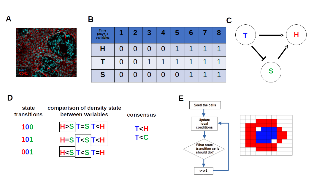
In this section, we present the methodological approach used for data inference and modeling. We shall highlight that the modeling process is contingent upon the outcomes derived from the inference. Figure 1 illustrates the workflow for data analysis and modeling. The source code link can be found at S4 Source code.

2.1. Experimental Data

We use previously published cell proliferation data measured in co-culture [1]. The data are the density ( c e l l s / m m 2 ) of normal human keratinocytes (HaCaT), metastatic melanoma (SK-MEL-147), at co-culture with the initial proportion of 1:10 (SK-MEL-147:HaCaT) [54] measured along 8 days in triplicate. To quantify the cell density necessary to achieve the carrying capacity, we introduced the variable S to express the difference between the carrying capacity (K) and the population density at each specific time point. This additional variable is justified because the space has a significant impact on the population dynamics. Hence, the more cells need to reach carrying capacity, less space is available, and the fewer cells need to reach carrying capacity, more space is available. Consequently, this variable serves as an initial arithmetic approximation of the space availability. Throughout this paper T will represent melanoma, H keratinocyte, and S space availability.

2.2. Boolean Network Inference

BN inference involves two steps: 1) binarization, which transforms cell counts per day in binary discrete data, and 2) network learning. We evaluated three different binarization methods: (1) k-means, (2) iterative k-means [10,55] and (3) BASC [56]. The binarization outcome chosen to network learning shall be the one which point highest density after confluence onset in agreement with Morais et al [1]. We used BoolNet 2.1.8 from R 4.2 [57] to implement the binarization by BASC and k-means, and Python 3.10.2 to implement the binarization by iterative k-means, adapted from Steinway et al [10]. In the context of this work, the number 0 denotes low density, and the number 1 denotes high density. We performed BN learning using the BestFit algorithm [58] through the BoolNet package 2.1.8 from R 4.2 [57].

2.3. Estimating the Agent-Based Models Rules from BN Basins through Consensus of State Transition Comparison

Here propose a simple method to estimate ABM rules from BN basin of attraction. The proposed approach involves two steps. First, we compare the density states among variables within state transitions belonging to a given basin of attraction and generate some sub-logic rules in term of inequalities. Second, we obtain a consensus about sub-logic rules among all state transitions belonging to the same basin of attraction. For instance, while analyzing six state transitions, it is observed that a specific variable A = 1 and variable B = 0 ( A B ) in three of them, while A = 0 and B = 1 ( A B ) in one of them, and A = 0 and B = 0 ( A = B ) in two of them. The most observed inequalities are A B and A = B , and we define the ABM rule as A B . We determine absence of regulation between variables when >, = and <, have the same frequencies such in case.

2.4. Implementation of Agent Based Model

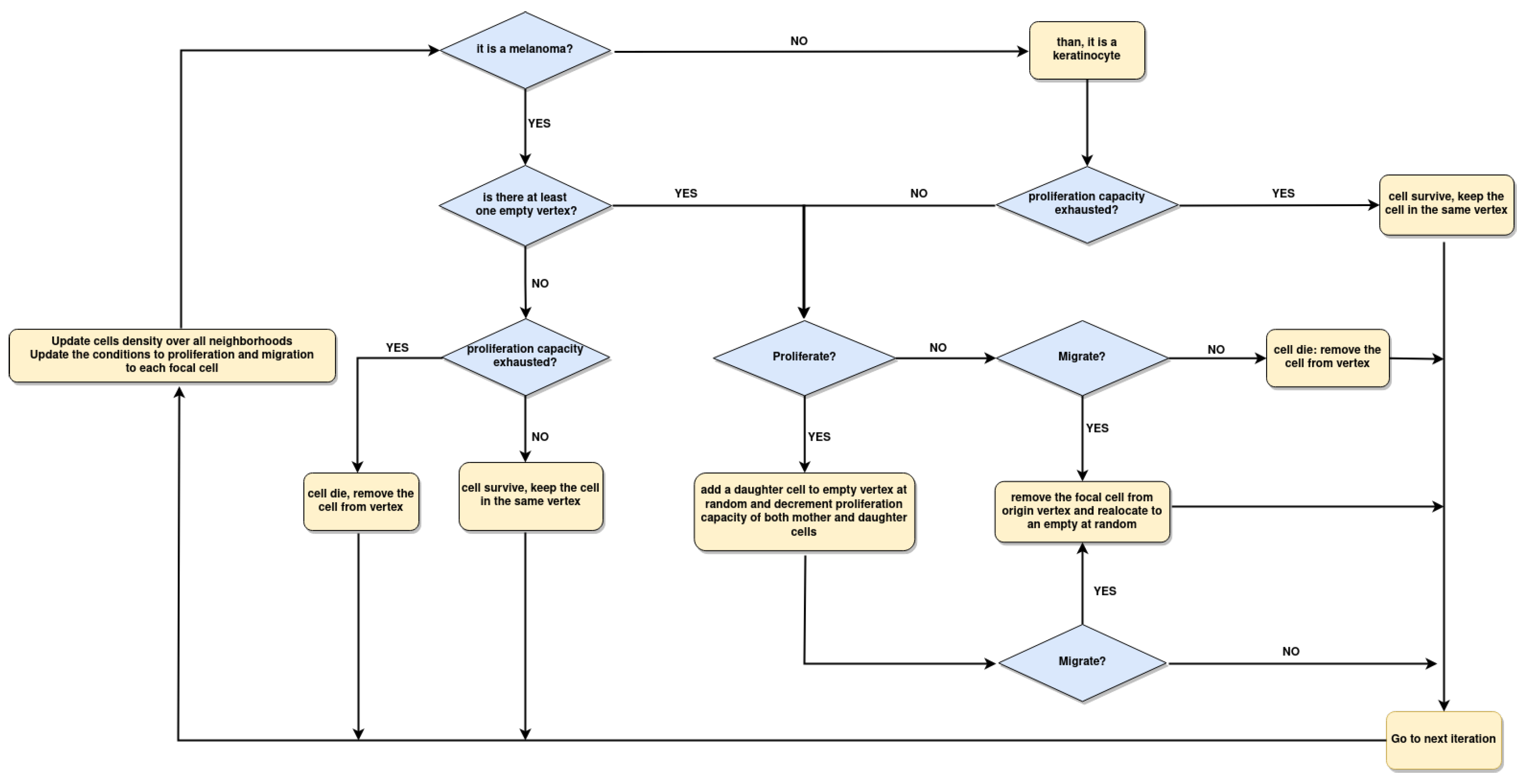
Among ABM classes we’ve implemented a SLCA which was built based on the estimation of growth dynamic rule from the BN basin (Figure 1). The model consists of a tissue scale, resulting in a single discrete variable, namely the cells. The model encompasses a dynamic process involving cell proliferation, death, migration, and survival. This process runs on a two-dimensional grid ( n × n with n = 200) with Moore neighborhood. The criteria for determining grid size was based on the spatial model developed by Morais et al [1]. Each vertex can accommodate only one tumor cell. During each iteration, all cells undergo the actions outlined in Figure 5. The cells were randomly distributed over the grid in a ratio of 1 T to 10 H according to [1]. We assume a time-step of 12 hours resulting in a total of 16 iteration, corresponding to 8 days-culture. Section 3.3 describes further detail about the state transition rules.

2.5. Spatial Configuration, Parameter Estimation, and Population Dynamics Process Probabilities

We applied a convolutional Gaussian filter of size k = 5 × 5 and standard deviation σ 2 to estimate the relative local density of H cells (arbitrary units) in the simulation domain. To calculate the growth curve of both cell lines we fitted the logistic model (Equation (1)) using the curve fit function of the optimize module of the Scipy library (version 1.7.1) in Python (version 3.10.2)
N ( t ) = K 1 e ρ ( t τ ) ,
where K denotes carrying capacity, ρ denotes proliferation rates and τ denotes time for half asymptote.
Throughout the simulations, we calculate the probability of the cells going through those tumor growth dynamic processes described in Section 2.4. Denote i = 1 , . . . , n as an element of the list ω = (Proliferation, Death, Migration, Survive) and f the frequency of occurrence of one of the processes in the list ω , thus
P r ( ω i ) = f ω i i = 1 n f ω i ,
for both T and H.

3. Results

3.1. The Iterative k-Means Binarization Method Demonstrated That Both Populations Are in High Density after 4 Days

As described in Section 2.2, the time series was binarized, and then we learned a BN. The binarization by iterative k-means showed a high density of H and T and a low availability of S, after four days (Figure 1 and in Figure S1).
Figure 2. The heatmap represents the binarization of co-culture time series by iterative k-means. The yellow cells represent 1, which means high density, and the blue cells represent 0, which means low density. Each row represents the binarized trajectories of H, T, and S, and each column represents the state transition of the network over eight days.
Preprints 89831 g002
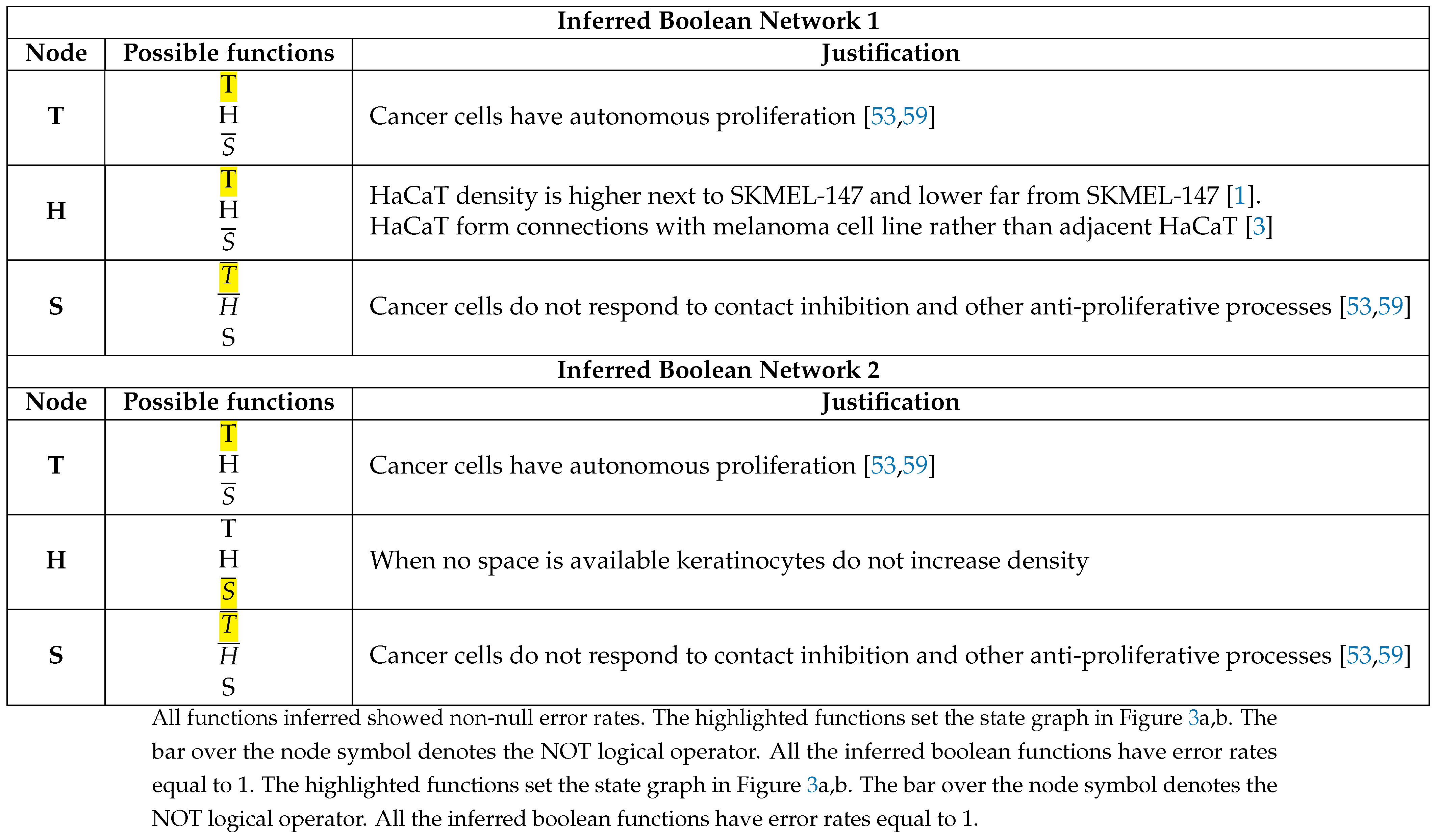
Table 1 shows the possible Boolean functions for each variable. The possible function for each variable is highlighted in yellow with its explanation. The intention of showing two different biologically reasonable networks is to ascertain possible plasticity in the estimated rules for ABM as the BN basin topologies change once a BN has 2 n possible state transitions, here n=3 (H, T, and S).

3.2. The Network Dynamics Exhibit Two Singleton Attractors

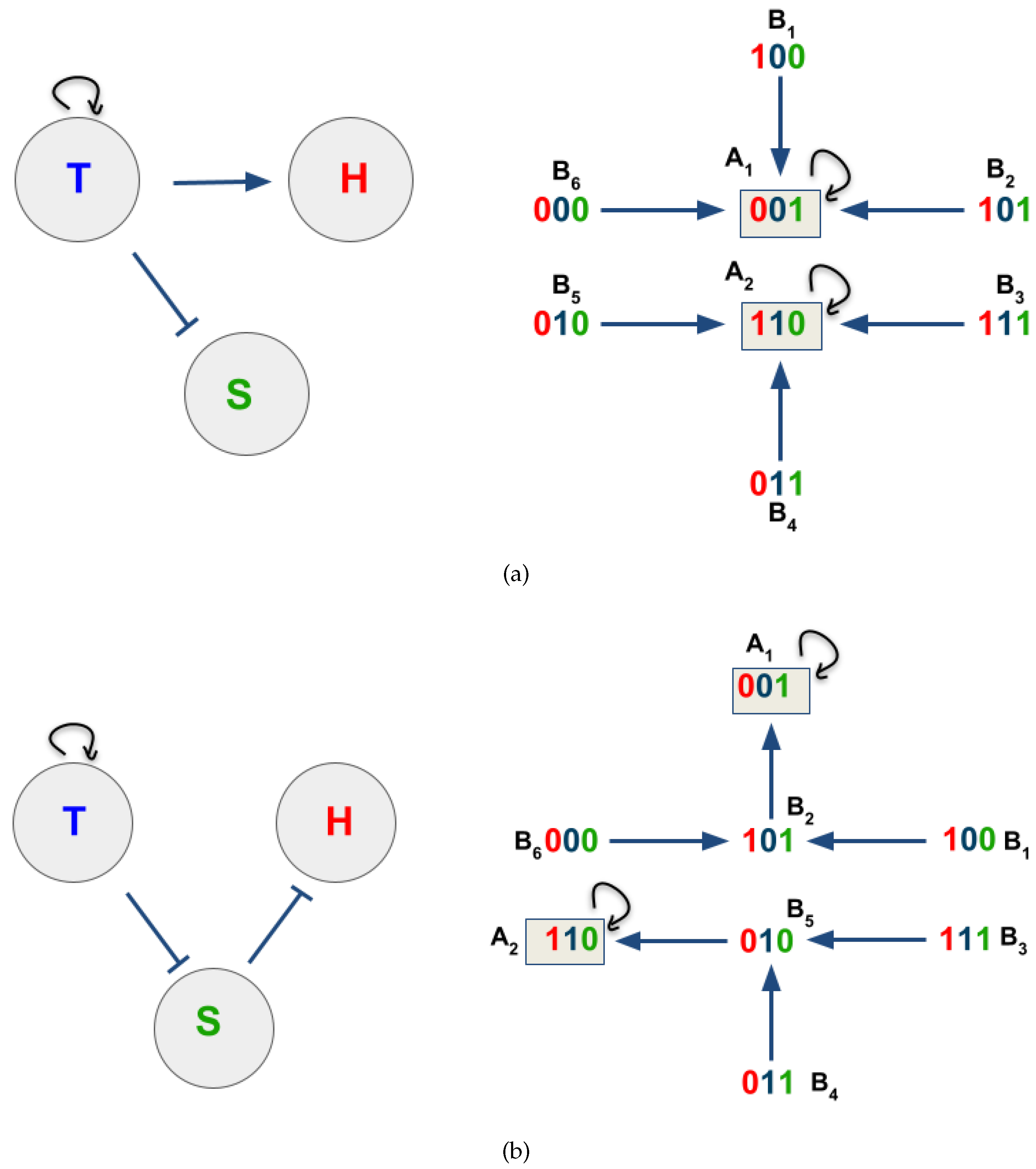
After we binarized the time series and applied a method of network learning, we generated the state graph, and observed two singletons (fix points) attractors in both IBN 1 (Figure 3a) and 2 (Figure 3b). Before evaluating the attractors and proceeding with the estimation of CA dynamics rules, we labeled each transition state as B 1 , B 2 , B 3 , B 4 , B 5 , B 6 , A 1 , A 2 . These IDs belongs to the same state transition in both IBN 1 and 2. The attractor A 1 shows T and H in low density, while S is in high density, which ultimately means high space availability or the population is scattered. The attractor A 2 shows H and T in high density and S in low density, which ultimately means low space availability or that the population is in high density. The IBN 1 has no predecessor state transition from initial condition among basins of attraction, while the IBN 2 present an small sequence of state transition not.

3.3. Boolean Network Basin Provide Growth Dynamic Rules for Proliferation and Migration

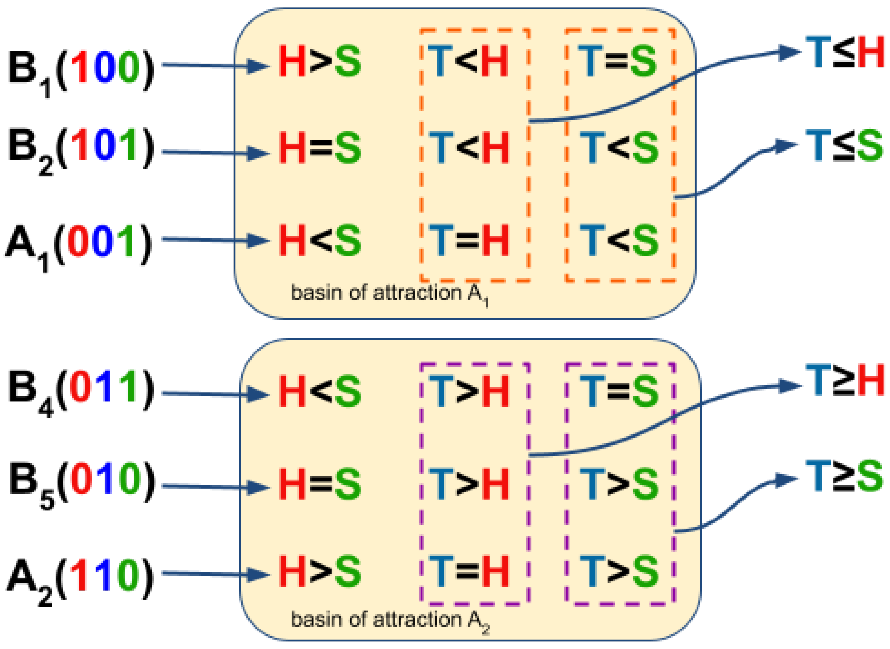
To estimate the growth dynamic rules to ABM from BN basin of attraction, we analyze the state transitions in terms of density state comparison. We ignore the state transitions that do not have a reasonable biological meaning considering a cell culture plate. B 3 presents a low cell density and low space availability, and B 6 presents a high cell density and high space availability. When we compare the density states between T and S among state transitions B 1 , B 2 , and A 1 , T < S is in two-thirds of these state transitions (orange-dash rectangle at Figure 4). Additionally, T < H is in 2/3 of the aforementioned state transitions (orange-dash rectangle at Figure 4). Thus, the consensus of the density state comparisons among these state transitions shows two inequalities: T S and T H (Figure 4). In contrast, upon comparing the density states between T and S among transition states B 4 , B 5 , and A 2 , T S is in two-thirds of these state transitions (purple-dash rectangle at Figure 4). Furthermore, T H is in 2/3 of those state transitions (purple-dash rectangle at Figure 4), so by consensus among these state transitions, we obtained two new inequalities: T S and T H (Figure 4).
The sub-logic rules T S and T H represent a condition in which there is a low amount of T and a high amount of H or S, which do not favor an increase in density, and according to [3], we determine that it favors migration. Thus, we set Equation (3) where M T , H denotes migration.
M T , H = ( T S ) ( T H )
The sub-logic rule T S and T H represent a condition where a higher density of T and a lower density H or S, favors density increase. Thus, P T and P H denotes proliferation of T and H in Equations (4) and (5), respectively. Due to the lack of data about the resources present in the cell culture media, we decided to augment Equations (4) and (5) with the probability of instantaneous proliferation 1 N K [60], since the logistic model fitted to the growth curves present in Morais et al [1]. If the probability of instantaneous proliferation is satisfied ( 1 N K r , where r is a random number) then the cells can proliferate. Another important condition to simulate cell dynamics is cell death, represented by the death term D ¯ T in Equation (4) and (5), and the survive term S V ¯ H that blocks H cell proliferation, as explained in Section 3.4.
P H = 1 N K ( ( T S ) ( T H ) ) S V ¯ H
P T = 1 N K ( ( T S ) ( T H ) ) D ¯ T

3.4. Data from Cell Lines and Growth Curves Allow Us to Propose an Intrinsic Rule to Describe Survival and Death of Each Agent
Here, we only could estimate a rule based in neighbors count that are compatible with migration and proliferation. Hence, we assigned an intrinsic rule to the agents survives or die. So in order to describe the survival and death of cells, we turn to Hayflick’s limit [61,62,63] concept to H and cancer stem cell hypothesis [64,65,66,67,68,69] to T because both can embrace the so-called parameter proliferation capacity ( ρ m a x ). Thus, with each cell division, the proliferation capacity of T and H will decrease by one unit, ρ m a x = ρ m a x 1 . It is well documented that H undergoes a limited number of duplications in the cell culture plate and does not always reach 100% confluence; thus, once H reaches ρ m a x = 0 , they survive ( S V H ), as proposed in Equation (6). We assume that when T reaches ρ m a x = 0 and in circumstances where there is no space ( D T ), the crowding situations might yield cell de-adherence and death [70], as in Equation (7).
S V H = ρ m a x = 0
D T = ρ m a x = 0 S = 0
Once H does not migrate, proliferate, or survive, they die, as in Equation (8). Alternately, once T does not migrate, proliferate, and die, they survive, Equation (9).
D H = M ¯ H P ¯ H S V ¯ H
S V T = M ¯ T D ¯ T P ¯ T
Figure 5. Flowchart of the ABM implementation. First, we set the initial density of cells and a random initial distribution of them over grid. At each iteration, the algorithm updates the amount of T, H, and empty vertex (S) in all focal cell neighborhoods. The conditions described in Equations (3) to (9) are updated in each cell. When there is at least one empty vertex, the cells proliferate or migrate, but when the proliferation capacity is exhausted, the cells survive or die.
Preprints 89831 g005

3.5. The Parameter Estimation Are in Agreement with Experimental Data

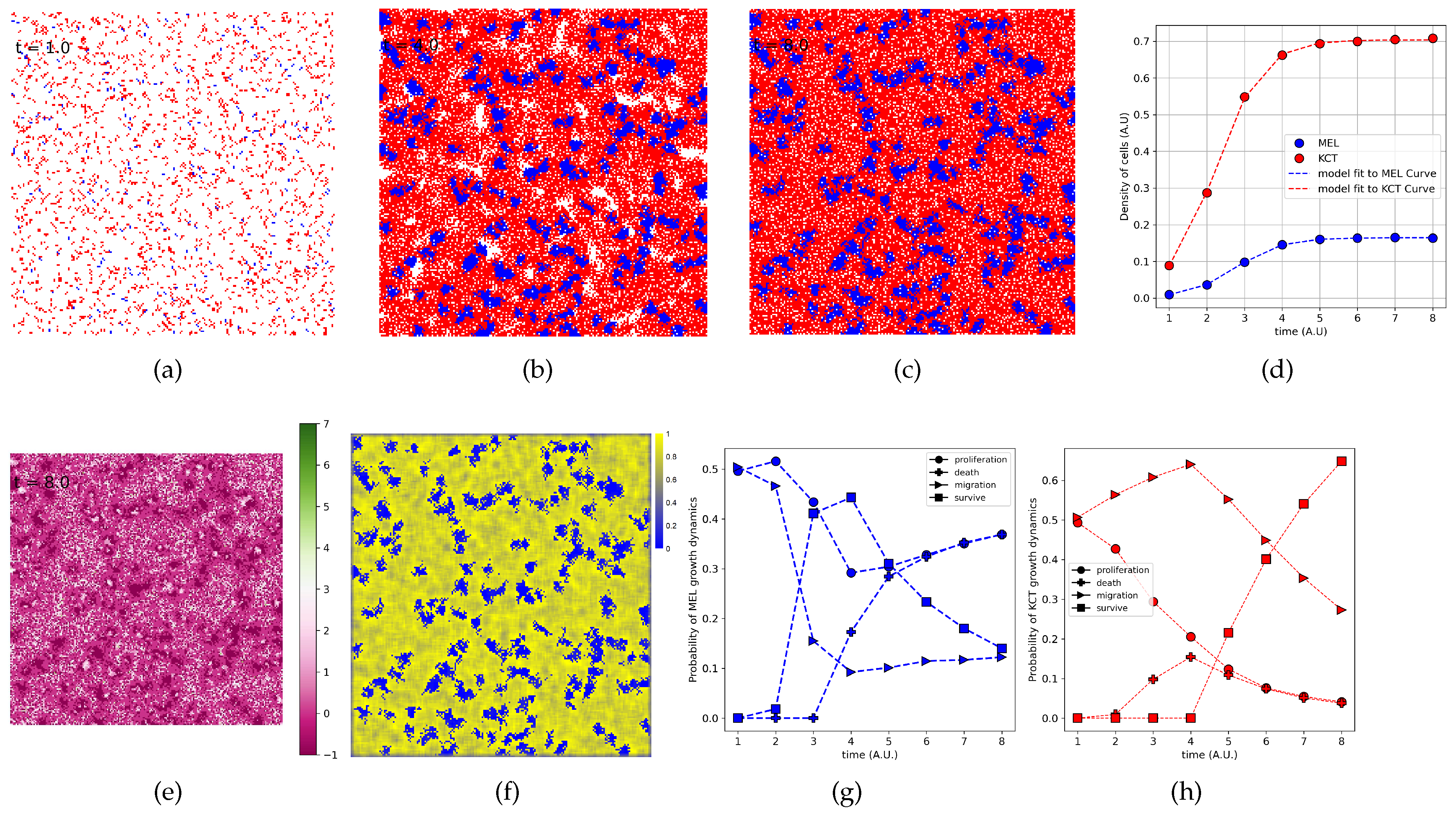
The values of cells density and the frequency of proliferating, migrating, surviving, and dying cell in the overall simulation were used to evaluate if the growth curve fit to the logistic model (Equation (1)). The growth curves fit the logistic model (Figure 6g) and the estimated values for the parameter K, ρ , and τ are presented at Table 2. Considering each iteration as a Δ t = 12 hours favored the estimation of ρ T ρ H and τ T τ H . We shall recall that the results in Figure 6 concern ρ m a x T = 7 and ρ m a x H = 6 . According to Morais et al [1] the values estimated to ρ T and ρ H are equal as well those estimated to τ T and τ H .

3.6. The Density of H Indeed Is Higher Close to T Cluster

We implemented the spatial model using ABM (Section 2.4, Section 3.3 and Section 3.4) and, starting from a given an initial distribution of cells. on the fourth day we can already see some T clusters surrounded by H, so this spatial pattern is consolidated on the eighth day (Figure 6a–c and animation in S3 Video). The heat map shows H density in the neighborhood of each focal cell (Figure 6f) points to higher yellow intensity around T clusters. This can be explained by the smooth increase in H migration probability from the beginning of the simulation (Figure 6(h)) as well as the increase in T survival probability from day 4 onward (Figure 6g). Therefore, as T clusters consolidate, more of the H neighborhood lacks T; hence the probability of migration decrease mostly because the probability of H survive increase substantially after four days (Figure 6(h)).

4. Discussion

In this study, we used the time series of the growth curve in the co-culture of T and H to infer a BN. Through BN inference, we were able to determine the boolean functions that led to network dynamics. These dynamics were shown in a state graph, where we arranged the state transitions according to the basin of attraction and estimated the ABM rules. These estimated rules were used in the implementation of an ABM to simulate spatial population dynamic. The binarization of the growth curve data reveals that the population attained a high density after 4 days. This observation aligns with the findings of Morais et al [1], who reported that the population achieves confluence after the same 4-day period. The proposed methodology captured the relationship between the confluence observed on the cell culture plate and the corresponding cell density. A boolean network of n nodes exhibits 2 n state transitions; hence, our time series, consisting of a sequence of 8 data points, can fully define the system. The occurrence of non-null error rates in the inferred boolean network arises due to the similarity of the H and T binarized trajectories, also known an identifiability, nevertheless, this issue can be solved by prior biological knowledge or by pruning the network nodes according to the context [39]. The BestFit BN learning paradigm searches for possible boolean functions that describe the state of a given variable (node) at time t + 1 as a function of the network state (the states of all nodes) at time t. In the heatmap (Figure 2), S is ON when both T and H are OFF, and vice versa, which means that S inhibits both T and H, which in turn inhibits S, and finally both T and H can "activate" each other. The IBN 1 in Table 1 and Figure 3a shows a canalizing node and a initial condition with no predecessor state transitons throughout basin of attraction. The IBN 2 in table Table 1 and Figure 3b, on the other hand, shows a small number of states before reaching the attractor. However, both networks (Figure 3a,b) have the same attractor. Hence, different BNs can lead to the same attractors. This indicates that the estimation of ABM rules was not affected by changes in the topology of the state graph, suggesting a system plastic capacity, as in the genetic networks [71]. Indeed melanoma affects keratinocytes phenotypes [2,3], our approach only captured an attractor state concerning local density of both melanoma and keratinocyte. By comparing the density states within state transitions B 4 , B 5 , and A 2 , we could estimate ( T S ) ( T H ) , suggesting that T will only proliferate where there is more T, since experiments with model organisms like zebrafish have shown that melanoma tends to cluster [72]. Likewise, we could estimate ( T S ) ( T H ) based on how the density states within states transition B 1 , B 2 , and A 1 , meaning that either H or T will move away [1,3]. It is worth highlighting that these Boolean expressions can be concurrently satisfied in a dynamic context, so the potential for cell proliferation and migration is inherently incorporated, which reduces any challenges in modeling associated with the go-or-grow phenomenon [73,74,75,76,77]. The spatial dynamic shows H more denser nearby T clusters than close to themselves (Figure 6a,b); moreover, the values estimated for ρ T , H and τ T , H are very similar. The value estimated to τ T , H is initial cell density-dependent and it is in agreement with [1]. The growth curve certainly did not emerge from the dynamics itself, but it is likely hardwired to the instantaneous probability term present in Equation (5) and (6) that was employed to represent the resources in the culture medium. Normal cells like H undergo a limited number of duplications in the cell culture plate and do not always reach 100% confluence because at each duplication the telomeres shorten, yielding to the onset of replicative senescence [61,62,63]. In the case of cancer cells, i.e., T, the telomeres shorten with doublings, and the cells will enter a state of crisis or death. Both normal and cancer cells could die whenever there is no space, because in vitro crowding situations lead some cells to undergo de-adherence and die [70]. Moreover, crowding-induced elimination facilitates the expansion of the malignant clones [78,79,80,81]. Due to the duration of the in vitro experiment (see Section 2.1) and for simplification, we discarded stem cells with ρ m a x = in the model. The proliferation capacity parameter ( ρ m a x ) as attribute to T death shows that cells with a lower ρ m a x value tend to be at the edges of the clusters, probably competing for space with cells with a higher ρ m a x value (Figure 6e). As soon as the cells on the periphery die, the others proliferate and thus decrease their proliferation capacity. In this respect, the ignition of stem cells by space freed and/or their capacity to proliferate more than those with no stemness are in agreement with previously published theoretical models [64,65,66,67,68,69], experimental evidence [82], and the amalgamation of experimental data with mathematical modeling [83,84]. The proliferation capacity as a simpler rule to distinguish death from survival allowed us to observe a decrease in the H:T density ratio (from 10:1 to 4:1) (Figure 6g). It is biologically sound because pathways involved in contact inhibition might go through a transition towards the regulation of autophagy, which in turn can yield survival and proliferation [85]. Hitherto, we could only estimate ABM rules for proliferation and migration and several intrinsic conditions of cells beyond proliferation capacity play an important role in survival and/or death. Probably, a time series with more variables or data points than ours could display more basins of attraction; in this manner, the rules for survival and death could be estimated. In doing so, if one can estimate the rules by which cells proliferate, migrate, die, and survive, an implementation of life-like CA become possible [7]. In that scenario, it would be possible to map the ABM dynamic backward through algorithms like those presented at the software DDLAB (www.ddlab.org) in order to evaluate the dynamic upon or on the network [44,49] and to develop a bioinformatic pipeline to evaluate if an ABM is chaotic or ordered as well gain insight about the path to system attractors. Despite this, here we propose a possibility of describe TME regulations in terms of a logical rules from the tumor growth curve, moreover, the logical rules ( T S ) ( T H ) and ( T S ) ( T H ) serves to define how neighborhood state cells drive population dynamics. Either model-driven experimentation or data-driven modeling is a key way to improve and combine mathematical, biological, and clinical models [86]. Concomitantly, a discrete approach can also be combined with a continuous one [87,88], and it is possible to estimate important parameters that go beyond how dynamics change locally or globally. Our approach deserves room for further refinement because cell co-culture is an experimental system where many data points can be obtained, as well as images of spatial patterns. This makes it much easier to explore networks at the tissue scale, especially when it comes to figuring out how to reconstruct population dynamics.

5. Conclusion

In this work, we introduce a novel approach to cell proliferation dynamics. We present a approach to estimate ABM rules from the basins of attraction of a Boolean network and, also, align them with experimental conditions. By establishing a direct connection between our theoretical model and experimentally observed spatial patterns, we attain a significant milestone in the field of cellular analysis by effectively connecting computation and experimental methods. This modeling approach can make a significant advancement in our ability to comprehend and predict complex biological phenomena.

Supplementary Materials

The following supporting information can be downloaded at the website of this paper posted on Preprints.org. Figure S1. Binarization heatmaps of both replicates and consensus of replicates according to different methods. The figures at the left side represent the binarization of replicates, and the figures at the right side represent the consensus of the binariztion. (A) BASC-A and k-means, (B) BASC-B, (C) iterative k-means. Figure S2. Probabilities of MEL growth dynamics according to the value assigned to (A) ρ m a x = 7. (B) ρ m a x = 8. (C) ρ m a x =5. Source code at github. Video S3. Animation of spatial population dynamic over time. GIF file with simulation frames. S4 Sorce Code. The source code can be found at the follow Github link. https://github.com/AlexandreSarmento/BooleanTumorGrowthKinetics.

Acknowledgments

We would like to thank NPAD/UFRN for computational resources. MCCM is supported by São Paulo State Research Foundation (FAPESP process n. 2020/12017-9). ASQ thanks Prof. Dr. Roger Chammas, who read the very first version of the article and assured him that the idea was coherent. Also ASQ thanks to Dr. Andrew Wuensche who gave him a feedback about the preprint version. The authors are thankful for anonymous reviewers whose comments enhanced manuscript’s quality.

References

  1. Morais MCC, Stuhl I, Sabino AU, Lautenschlager WW, Queiroga AS, Tortelli Jr TC, et al. Stochastic model of contact inhibition and the proliferation of melanoma in situ. Sci Rep. 2017; 7: 8026. [CrossRef]
  2. Kodet O, Lacina L, Krejčí E, Dvořánková B, Grim M, Štork J, et al. Melanoma cells influence the differentiation pattern of human epidermal keratinocytes. Mol Cancer. 2015; 14: 1-12. [CrossRef]
  3. Mazurkiewicz J, Simiczyjew A, Dratkiewicz E, Kot M, Pietraszek-Gremplewicz K, Wilk D, et al. Melanoma stimulates the proteolytic activity of HaCaT keratinocytes. Cell Commun Signal. 2022; 20: 1-17. [CrossRef]
  4. Garcia, JM. Agent-based Modeling and Simulation. Amazon Digital Service: Seattle; 2021.
  5. Neumann JV. Theory of self-reproducing automata. Edited by Arthur WBurks. 1966.
  6. Wolfram S. Statistical mechanics of cellular automata. Rev Mod Phys. 1983; 55: 601. [CrossRef]
  7. Gardner, M. Mathematical Games The fantastic combinations of John Conway’s new solitaire game ’life’. Scientific American 223. pp. 120–123, 1970.
  8. Kauffman S. Homeostasis and differentiation in random genetic control networks. Nature. 1969; 224: 177-178. [CrossRef]
  9. Bornholdt S. Boolean network models of cellular regulation: prospects and limitations. J R Soc Interface. 2008; 5: 85-94. [CrossRef]
  10. Steinway SN, Biggs MB, Loughran Jr TP, Papin JA, Albert R. Inference of network dynamics and metabolic interactions in the gut microbiome. PLoS Comput Biol. 2015; 11: e1004338. [CrossRef]
  11. Claussen JC, Skiecevičienė J, Wang J, Rausch P, Karlsen TH, Lieb W, Baines JF, Franke A, Hütt MT. Boolean analysis reveals systematic interactions among low-abundance species in the human gut microbiome. PLoS Comput Biol. 2017;13:e1005361. [CrossRef]
  12. Dormann S, Deutsch A. Modeling of self-organized avascular tumor growth with a hybrid cellular automaton. In Silico Biol. 2002; 2: 393-406.
  13. Spencer SL, Gerety RA, Pienta KJ, Forrest S. Modeling somatic evolution in tumorigenesis. PLoS Comput Biol. 2006; 2: 108. [CrossRef]
  14. Enderling H, Hlatky L, Hahnfeldt P. Migration rules: tumours are conglomerates of self-metastases. Br J Cancer. 2009; 100: 1917-1925. [CrossRef]
  15. Enderling H, Anderson AR, Chaplain MA, Beheshti A, Hlatky L, Hahnfeldt P. Paradoxical dependencies of tumor dormancy and progression on basic cell kinetics. Cancer Res. 2009; 69: 8814-8821. [CrossRef]
  16. Kansal A, Torquato S, Chiocca E, Deisboeck T. Emergence of a subpopulation in a computational model of tumor growth. J Theor Biol. 2000; 207: 431-441. [CrossRef]
  17. Zhang L, Strouthos CG, Wang Z, Deisboeck TS. Simulating brain tumor heterogeneity with a multiscale agent-based model: linking molecular signatures, phenotypes and expansion rate. Mathematical and computer modelling. 2009; 49: 307-319. [CrossRef]
  18. Wcisło R, Dzwinel W, Yuen DA, Dudek AZ. A 3-D model of tumor progression based on complex automata driven by particle dynamics. J Mol Mod 2009; 15: 1517-1539. [CrossRef]
  19. Wang Z, Deisboeck TS. Computational modeling of brain tumors: discrete, continuum or hybrid? Sci Mod Sim. 2009; 381–393. [CrossRef]
  20. Anderson AR, Rejniak KA, Gerlee P, Quaranta V. Microenvironment driven invasion: a multiscale multimodel investigation. J Math Biol. 2009; 58: 579-624. [CrossRef]
  21. Zhang L, Wang Z, Sagotsky JA, Deisboeck TS. Multiscale agent-based cancer modeling. J Math Biol. 2009; 58: 545–559. [CrossRef]
  22. Anderson AR. A hybrid mathematical model of solid tumour invasion: the importance of cell adhesion. Math Med Biol. 2005; 22: 163-186. [CrossRef]
  23. Sottoriva A, Verhoeff JJ, Borovski T, McWeeney SK, Naumov L, Medema JP, et al. Cancer stem cell tumor model reveals invasive morphology and increased phenotypical heterogeneity. Cancer Res. 2010; 70: 46-56. [CrossRef]
  24. Gatenby RA, Smallbone K, Maini PK, Rose F, Averill J, Nagle RB, et al. Cellular adaptations to hypoxia and acidosis during somatic evolution of breast cancer. Br J Cancer. 2007; 97: 646-653. [CrossRef]
  25. Gerlee P, Anderson A. Evolution of cell motility in an individual-based model of tumour growth. J Theor Biol. 2009; 259: 67-83. [CrossRef]
  26. Silva AS, Yunes JA, Gillies RJ, Gatenby RA. The potential role of systemic buffers in reducing intratumoral extracellular pH and acid-mediated invasion. Cancer Res. 2009; 69: 2677-2684. [CrossRef]
  27. Zhang L, Chen LL, Deisboeck TS. Multi-scale, multi-resolution brain cancer modeling. Math Comput Simul. 2009; 79: 2021-2035. [CrossRef]
  28. Gerlee P, Anderson AR. A hybrid cellular automaton model of clonal evolution in cancer: the emergence of the glycolytic phenotype. J Theor Biol. 2008; 250: 705-722. [CrossRef]
  29. Smallbone K, Gatenby RA, Gillies RJ, Maini PK, Gavaghan DJ. Metabolic changes during carcinogenesis: potential impact on invasiveness. J Theor Biol. 2007; 244: 703-713. [CrossRef]
  30. Anderson AR, Hassanein M, Branch KM, Lu J, Lobdell NA, Maier J, et al. Microenvironmental independence associated with tumor progression. Cancer Res. 2009; 69: 8797-8806. [CrossRef]
  31. Anderson AR, Weaver AM, Cummings PT, Quaranta V. Tumor morphology and phenotypic evolution driven by selective pressure from the microenvironment. Cell. 2006; 127: 905-915. [CrossRef]
  32. Basanta D, Strand DW, Lukner RB, Franco OE, Cliffel DE, Ayala GE, et al. The role of transforming growth factor-β–mediated tumor-stroma interactions in prostate cancer progression: An integrative approach. Cancer Res. 2009; 69: 7111-7120.
  33. de Pillis LG, Mallet DG, Radunskaya AE. Spatial tumor-immune modeling. Comput Math Methods Med. 2006;7: 159-176. [CrossRef]
  34. Enderling H, Alexander NR, Clark ES, Branch KM, Estrada L, Crooke C, et al. Dependence of invadopodia function on collagen fiber spacing and cross-linking: computational modeling and experimental evidence. Biophys J. 2008; 95: 2203-2218.
  35. Bankhead A, Magnuson NS, Heckendorn RB. Cellular automaton simulation examining progenitor hierarchy structure effects on mammary ductal carcinoma in situ. J Theor Biol. 2007; 246: 491-498. [CrossRef]
  36. Gevertz J, Torquato S. Growing heterogeneous tumors in silico. Phys Rev E. 2009;80: 51-91. [CrossRef]
  37. Anderson AR, Basanta D, Gerlee P, Rejniak KA. Evolution, regulation, and disruption of homeostasis, and its role in carcinogenesis. Multiscale Cancer Modeling. Boca Raton: Taylor and Francis; 2011. pp. 1–30.
  38. Silva AS, Gatenby RA, Gillies RJ, Yunes JA. A quantitative theoretical model for the development of malignancy in ductal carcinoma in situ. J Theor Biol. 2010; 262: 601-613. [CrossRef]
  39. Putnins M, Campagne O, Mager D, Androulakis I. From data to QSP models: a pipeline for using Boolean networks for hypothesis inference and dynamic model building. J Pharmacokinet Pharmacodyn. 2022; p. 1–15.
  40. Schlatter R, Schmich K, Avalos Vizcarra I, Scheurich P, Sauter T, Borner C, et al. ON/OFF and beyond-a Boolean model of apoptosis. PLoS Comput Biol. 2009; 5: e1000595. [CrossRef]
  41. Mai Z, Liu H. Boolean network-based analysis of the apoptosis network: irreversible apoptosis and stable surviving. J Theor Biol. 2009; 259: 760-769. [CrossRef]
  42. Steinway SN, Zañudo JG, Ding W, Rountree CB, Feith DJ, Loughran Jr TP, et al. Network modeling of TGFβ signaling in hepatocellular carcinoma epithelial-to-mesenchymal transition reveals joint sonic hedgehog and Wnt pathway activation. Cancer Res. 2014; 74: 5963-5977.
  43. Fumia HF, Martins ML. Boolean network model for cancer pathways: predicting carcinogenesis and targeted therapy outcomes. PLoS One. 2013; 8: e69008. [CrossRef]
  44. Wuensche A, Lesser M. Global dynamics of cellular automata: An atlas of basin of attraction fields of one-dimensional cellular automata. vol 1. Colorado: Westview Press; 1992.
  45. Voorhees B Predecessors of cellular automata states II. Pre-images of finite sequences. Physica D. 1994;73 :136-151.
  46. Wuensche A. Attractor basins of discrete networks. Cogn Sci Res Paper. 1997; 461.
  47. Jeras I, Dobnikar A. Algorithms for computing preimages of cellular automata configurations. Physica D. 2007; 233: 95-111. [CrossRef]
  48. Soto JMG. Computation of explicit preimages in one-dimensional cellular automata applying the De Bruijn diagram. J Cell Autom. 2008; 3: 219-230.
  49. Wuensche A. Exploring discrete dynamics. 1st ed. United Kingdom: Luniver Press; 2011.
  50. West J, Newton PK. Cellular interactions constrain tumor growth. Proc Natl Acad Sci U S A. 2019;116: 1918-1923. [CrossRef]
  51. Quail DF, Joyce JA. Microenvironmental regulation of tumor progression and metastasis. Nature medicine. 2013; 19: 1423-1437. [CrossRef]
  52. Maley CC, Aktipis A, Graham TA, Sottoriva A, Boddy AM, Janiszewska M, et al. Classifying the evolutionary and ecological features of neoplasms. Nat Rev Cancer. 2017;17 : 605-619. [CrossRef]
  53. Hanahan D. Hallmarks of cancer: new dimensions. Cancer Discov. 2022; 12: 31-46. [CrossRef]
  54. Cichorek M, Wachulska M, Stasiewicz A, Tymińska A. Skin melanocytes: biology and development. Postepy Dermatol Alergol. 2013; 30: 30-41.
  55. Berestovsky N, Nakhleh L. An evaluation of methods for inferring boolean networks from time-series data. PLoS One. 2013; 8: e66031. [CrossRef]
  56. Hopfensitz M, Mussel C, Wawra C, Maucher M, Kuhl M, Neumann H, et al. Multiscale binarization of gene expression data for reconstructing Boolean networks. IEEE/ACM Trans Comput Biol Bioinform. 2011; 9: 487-498. [CrossRef]
  57. Müssel C, Hopfensitz M, Kestler HA. BoolNet—an R package for generation, reconstruction and analysis of Boolean networks. Bioinform. 2010;26(10):1378–1380. [CrossRef]
  58. Lähdesmäki H, Shmulevich I, Yli-Harja O. On learning gene regulatory networks under the Boolean network model. Mach Learn. 2003; 52: 147–167. [CrossRef]
  59. Weinberg RA. The biology of cancer. WW Norton and Company. 2013.
  60. Benzekry S, Lamont C, Beheshti A, Tracz A, Ebos JM, Hlatky L, et al. Classical mathematical models for description and prediction of experimental tumor growth. PLoS Comput Biol. 2014;10: e1003800. [CrossRef]
  61. Hayflick L, Moorhead PS. The serial cultivation of human diploid cell strains. Exp Cell Res. 1961;25: 585-621. [CrossRef]
  62. Hayflick L. The limited in vitro lifetime of human diploid cell strains. Exp Cell Res. 1965; 37: 614-636. [CrossRef]
  63. Blackburn EH, Gall JG. A tandemly repeated sequence at the termini of the extrachromosomal ribosomal RNA genes in Tetrahymena. J Mol Biol. 1978; 120: 33-53. [CrossRef]
  64. Poleszczuk J, Hahnfeldt P, Enderling H. Biphasic modulation of cancer stem cell-driven solid tumour dynamics in response to reactivated replicative senescence. Cell Prolif. 2014; 47: 267-76. [CrossRef]
  65. Poleszczuk J, Enderling H. A high-performance cellular automaton model of tumor growth with dynamically growing domains. Appl. Math. 2014; 5: 144-152. [CrossRef]
  66. Poleszczuk J, Hahnfeldt P, Enderling H. Evolution and phenotypic selection of cancer stem cells. PLoS Comput Biol. 2015; 11: e1004025. [CrossRef]
  67. Poleszczuk J, Enderling H. Cancer stem cell plasticity as tumor growth promoter and catalyst of population collapse. Stem Cells Int. 2016;2016. [CrossRef]
  68. Morton CI, Hlatky L, Hahnfeldt P, Enderling H. Non-stem cancer cell kinetics modulate solid tumor progression. Theor Biol Med Model. 2011; 8:1-13. [CrossRef]
  69. Shyntar A, Patel A, Rhodes M, Enderling H, Hillen T. The Tumor Invasion Paradox in Cancer Stem Cell-Driven Solid Tumors. Bull Math Biol. 2022; 84 :139. [CrossRef]
  70. Topman G, Sharabani-Yosef O, Gefen A. A method for quick, low-cost automated confluency measurements. Microsc Microanal. 2011; 17: 915-922. [CrossRef]
  71. Martin S, Zhang Z, Martino A, Faulon JL. Boolean dynamics of genetic regulatory networks inferred from microarray time series data. Bioinform. 2007; 23: 866-874. [CrossRef]
  72. Campbell NR, Rao A, Hunter MV, Sznurkowska MK, Briker L, Zhang M, et al. Cooperation between melanoma cell states promotes metastasis through heterotypic cluster formation. Dev Cell. 2021; 56: 2808-2825. [CrossRef]
  73. Hatzikirou H, Basanta D, Simon M, Schaller K, Deutsch A. ‘Go or grow’: the key to the emergence of invasion in tumour progression? Math Med Biol. 2012; 29: 49-65.
  74. Gallaher J, Anderson AR. Evolution of intratumoral phenotypic heterogeneity: the role of trait inheritance. Interface Focus. 2013; 3: 20130016. [CrossRef]
  75. Kimmel GJ, Dane M, Heiser LM, Altrock PM, Andor N. Integrating mathematical modeling with high-throughput imaging explains how polyploid populations behave in nutrient-sparse environments. Cancer Res. 2020; 80: 5109-5120. [CrossRef]
  76. Garay T, Juhász É, Molnár E, Eisenbauer M, Czirók A, Dekan B, et al. Cell migration or cytokinesis and proliferation?–revisiting the “go or grow” hypothesis in cancer cells in vitro. Exp Cell Res. 2013; 319: 3094-3103.
  77. Vittadello ST, McCue SW, Gunasingh G, Haass NK, Simpson MJ. Examining go-or-grow using fluorescent cell-cycle indicators and cell-cycle-inhibiting drugs. Biophys J. 2020; 118: 1243-1247. [CrossRef]
  78. Kon S, Ishibashi K, Katoh H, Kitamoto S, Shirai T, Tanaka S, et al. Cell competition with normal epithelial cells promotes apical extrusion of transformed cells through metabolic changes. Nat Cell Biol. 2017; 19: 530-541. [CrossRef]
  79. Hill W, Zaragkoulias A, Salvador-Barbero B, Parfitt GJ, Alatsatianos M, Padilha A, et al. EPHA2-dependent outcompetition of KRASG12D mutant cells by wild-type neighbors in the adult pancreas. Curr Biol. 2021; 31: 2550-2560. [CrossRef]
  80. Martins VC, Busch K, Juraeva D, Blum C, Ludwig C, Rasche V, et al. Cell competition is a tumour suppressor mechanism in the thymus. Nature. 2014; 509: 465-470. [CrossRef]
  81. Wagstaff L, Goschorska M, Kozyrska K, Duclos G, Kucinski I, Chessel A, et al. Mechanical cell competition kills cells via induction of lethal p53 levels. Nature Commun. 2016; 7: 11373. [CrossRef]
  82. Alowaidi F, Hashimi SM, Alqurashi N, Alhulais R, Ivanovski S, Bellette B, et al. Assessing stemness and proliferation properties of the newly established colon cancer ‘stem’cell line, CSC480 and novel approaches to identify dormant cancer cells. Oncol Rep. 2018; 39: 2881-2891.
  83. Gao X, McDonald JT, Hlatky L, Enderling H. Acute and fractionated irradiation differentially modulate glioma stem cell division kinetics. Cancer Res. 2013; 73: 1481-1490. [CrossRef]
  84. Tang J, Fernandez-Garcia I, Vijayakumar S, Martinez-Ruis H, Illa-Bochaca I, Nguyen DH, et al. Irradiation of juvenile, but not adult, mammary gland increases stem cell self-renewal and estrogen receptor negative tumors. Stem Cells. 2014; 32: 649-661. [CrossRef]
  85. Pavel M, Renna M, Park SJ, Menzies FM, Ricketts T, Füllgrabe J, et al. Contact inhibition controls cell survival and proliferation via YAP/TAZ-autophagy axis. Nature Commun. 2018; 9: 2961.
  86. Enderling, H., Wolkenhauer, O. Are all models wrong? Comput Sys Oncol. 2020; 1: e1008.
  87. Wittmann DM, Krumsiek J, Saez-Rodriguez J, Lauffenburger DA, Klamt S, Theis FJ. Transforming Boolean models to continuous models: methodology and application to T-cell receptor signaling. BMC Syst Biol. 2009; 3: 1-21. [CrossRef]
  88. Krumsiek J, Pölsterl S, Wittmann DM, Theis FJ. Odefy-from discrete to continuous models. BMC Bioinform. 2010;11: 1-10. [CrossRef]
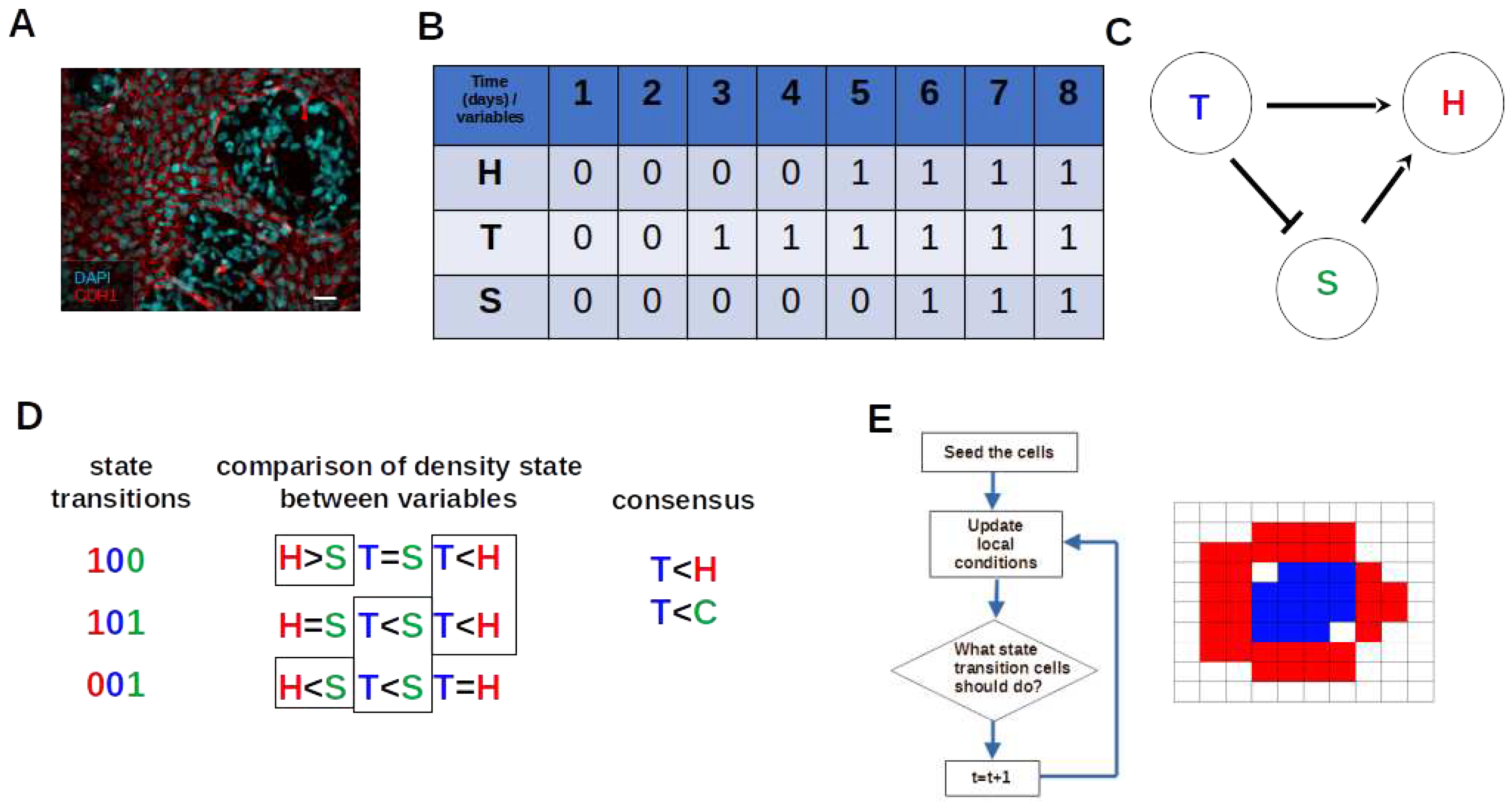
Figure 1. Workflow of data inference and population dynamic modeling. (A) Cell co-culture model of keratinocytes and melanoma cells Scale bar: 50 μ m [1]. (B) Population growth time-series binarization. Number 0 indicates a low density of cells (OFF state), and number 1 indicates a high density of cells (ON state). (C) Inferred Boolean Network Topology Arrows indicate activation and blunt arrows indicate inhibition. (D) Estimating ABM rules through comparing variable density state within state transitions and among them. (E) Implementation of simulation through cellular automata.
Preprints 89831 g001
Figure 3. The dynamics of IBN 1 and 2. (A) the topology of the network is shown on the left, and the state graph of IBN 1 on the right. (B) The topology of the network is shown on the left, and the state graph of IBN 2 on the right. A 1 and A 2 denote singleton attractors 1 and 2, respectively, and the letter B denotes state transitions. The red number represents the density state of H, the blue number represents the density state of T, and the green number, the space availability state of S.
Preprints 89831 g003
Figure 4. Estimate of the ABM dynamic rule from the BN basin. One can observe the comparison within each state transition ( B 1 , B 2 , B 4 , B 5 , A 1 and A 2 ) where the number in red indicating the density state of H, blue indicating T, and green indicating S. The dashed rectangles marks the sub-logic rules coming from comparisons among state transitions belonging to a basin of attraction, and the arrow points to the consensus of the sub-logic rules among state transitions. The orange-dash rectangle concerns the basin of attraction A 1 , while the purple-dash rectangle to A 2 .
Preprints 89831 g004
Figure 6. The spatial population and tumor growth dynamics. (A), (B), and (C) frames correspond to days 1, 4, and 8. Blue represents T, and red represents H. (D) Growth curves of T and H. E Spatial distribution of the cells according to the values of ρ m a x at day 8. In the bar of color at right, the shades of green to pink represent the ρ m a x values. (F) Heatmap representing H density over all focal cell neighborhoods at day 8. In the bar of color at right, the shades of blue to yellow represent the percentage of occupied vertex by H in all focal cell neighborhoods. (G) Probabilities of T tumor growth dynamics (H) Probabilities of H tumor growth dynamics.
Preprints 89831 g006
Table 1. Inferred boolean functions through the Best Fit algorithm.
Preprints 89831 i001
Table 2. Table of estimated values for the parameters of the logistic model.
Preprints 89831 i002
Disclaimer/Publisher’s Note: The statements, opinions and data contained in all publications are solely those of the individual author(s) and contributor(s) and not of MDPI and/or the editor(s). MDPI and/or the editor(s) disclaim responsibility for any injury to people or property resulting from any ideas, methods, instructions or products referred to in the content.
Copyright: This open access article is published under a Creative Commons CC BY 4.0 license, which permit the free download, distribution, and reuse, provided that the author and preprint are cited in any reuse.
Prerpints.org logo

Preprints.org is a free preprint server supported by MDPI in Basel, Switzerland.

Subscribe

© 2024 MDPI (Basel, Switzerland) unless otherwise stated