Stochastic Claims Reserve in the Healthcare System: A New Methodology Applied in Italy

One of the challenges in the healthcare sector is making accurate forecasts across insurance years for claims reserve. The state-of-the-art envisages various methods for estimating the claims reserve but without being applied to systems that do not present huge variability and heterogeneity, such as the healthcare sector. The methodology is based on generalized linear models using the Overdispersed Poisson distribution as shown in the state-of-the-art. In this context, we developed a method to estimate the parameters of the quasi-likelihood function using a Gauss-Newton algorithm optimized through a genetic algorithm. The genetic algorithm plays a crucial role in glimpsing the position of the global minimum to ensure a correct convergence of the Gauss-Newton method, where the choice of the initial guess is fundamental. The proposed methodology has been entirely developed using MATLAB and has been applied to estimate the claims reserve in the healthcare system of the Tuscany Region in Italy, as case study. The results obtained were validated by comparing them with the state-of-the-art by measuring the confidence intervals of the Overdispersed Poisson distribution parameters. Therefore local healthcare authorities could use the proposed and improved methodology to allocate the resources dedicated to healthcare and global management.

Keywords:

Subject: Business, Economics and Management - Econometrics and Statistics

1. Introduction

1.1. The medical malpractice in Italy: liability rule and definition of claims reserve

The term “medical malpractice” is intended to define those damages (tending to be biological, but also in perspective moral) arising from errors in the health sector of the practitioner and closely related to clinical activity in the strict sense [1]. This damage is closely correlated with civil liability in healthcare, which profoundly impacts the economy and society. Indeed, the healthcare expenditure was estimated for 2019 at 8.7% of the national Gross Domestic Product (GDP), which is below the EU average of 9.9% [3]. It should be noted that approximately 15% of hospital expenditure in high-income countries is used to correct complications of care and patient harm [2]. Although in these countries with an efficient healthcare system, adverse events seem to be progressively decreasing. It is estimated that 10% of patients experience an adverse event during medical-surgical treatment, resulting in a malpractice injury. The most frequently reported types of adverse events, on a global level, undoubtedly include surgical procedures - with significant peaks among orthopaedics and traumatology, general surgery and obstetrics and gynaecology [6] - diagnostic errors, accidental falls, and the contraction of nosocomial infections, in reference to which specific investigation would be due. In Italy, no official national published statistics on medical adverse events and/or claims exist. However, some regions have published independent reports on hospital claims in the past, showing that most complaints are received in the above-mentioned operational areas [18,24]. When an adverse event occurs, Italian healthcare liability is imposed on healthcare organizations and, potentially, healthcare professionals who committed the error. Healthcare public and private institutions are liable with contractual liability for the behaviour of healthcare professionals whose services they employ, with reference to professionals, including researchers, under any contract of the National Health Service. For this reason, public and private health and social care facilities must be provided with insurance coverage or other similar measures for third parties’ liability and towards employees. Other measures include the possibility for organizations to constitute cover funds from internal provisions to protect all or part of the health liability risk. The amount of money to pay insurance premiums or to provide coverage funds derives from the national health fund, which is then distributed to the different regions. In turn, they may distribute the money to their health organizations or centralize the resources to shield against claims. Therefore, insurance or self-insurance coverage must be provided to be operative in the event of a medical malpractice claim. However, given the significant fluctuation in medical malpractice claims, the challenge arises regarding how much money should be allocated annually to guarantee the fulfilment of its financial commitments and the payment of compensation for damages. In this study, the authors aim to address the following research questions: 1) Which models are appropriate for estimating claims reserves in the healthcare sector? 2) How can the models be adapted to enhance the state-of-the-art (SoA) models to fit our specific context?

The proposed work can be positioned in the context described above to build a solid procedure to estimate and manage the claims reserve. The treatment developed here will be technical because the authors want to provide a complete mathematical and computational tool for the healthcare system to allocate appropriate resources. The paper is organized as follows: 1) the first part is focused on the mathematical background behind the GLM to underline the foundation of the applied methodology, jointly with the definition of the quasi-likelihood function to model the response variables, as well as the algorithms to locate the best parameters that maximize these function and the corresponding errors associated to the parameters of the quasi-likelihood function; 2) the second part of the work is focused on the validation of the developed models by providing a detailed comparison with the present SoA, based on the confidence intervals of the parameters that maximize the quasi-likelihood function; 3) in the third-last part, the authors illustrate an application of the developed methodology to the disposable data coming from Tuscany Region1 to show its capability compared to the available SoA; 4) finally, discussion and conclusions are provided with improvements and future development. All the numerical analyses and computations described in this work have been implemented with the Matlab software package.

1.2. Structure and main ideas

The Generalized Linear Model (GLM) in the last few years has become a significant reality in claims reserve analysis [7,8,14,15,25]. The present work supplies the context of their forecast and applicability. The authors found the necessity, at first, to better describe and elucidate the mathematical background inside the subject and to assemble a coherent and well-defined model. In this context, the authors contributed to creating a new framework that could provide adequate and complete results in claims reserve.

The basis to estimate the claims reserve is through the construction of the Run-Off triangles [20] that estimate the total paid amount of claims incurred that are not yet reported to the insurance agency. A common methodology to estimate claims reserve is the Chain-Ladder (CL) [12,21,26]. The CL method aims to approximate the value of claims reserves that have been incurred but not yet reported and to predict the ultimate loss amounts in general insurance. The fundamental assumption on which the CL is based is that the patterns observed in historical loss development must hold for future loss development. The previous assumption represents one of the limitations of the CL and other deterministic methods because they do not extrapolate the tail factors [8] to increase the prediction performance for the paid amount. Several modifications of the CL have been proposed in the literature to improve the prediction of the claims reserve [11,23], and various stochastic claim reserving models have been developed for the general insurance to extrapolate the tail factors.

The employment of the stochastic models replicates the conventional reserve estimates produced by the CL methods, including parametric curves and smoothing techniques to reshape the runoff triangles, enabling the estimation of the tail factors through extrapolation. Stochastic models offer a significant benefit in providing precision measures for claims reserve, particularly emphasising the mean squared error of the prediction. However, understanding the stochastic distribution function of the claims reserve outcome is crucial to provide good prediction performances [19]. In this regard, the GLM has become, in the last years, a robust stochastic methodology for predicting claims reserve [12,17]. The GLM represents a wide range of models that allow the definition and estimation of parameters by maximising the likelihood function [17]. In this framework, the likelihood function is employed to evaluate the goodness of fit for a distribution that belongs to the exponential family of random variables. To define the likelihood function, one must specify the analytical form of the response variable distribution. In the works of [27,28], the last assumption has been overcome by introducing the quasi-likelihood function, which only needs the definition of the mean-variance relation of the response variable without any assumption on the shape of its distribution. Following the work of [22], the authors assume a logarithmic mean-variance relation, which provides the well-known over-dispersed Poisson (ODP) distribution model. The maximisation of the ODP quasi-likelihood function is performed using the Gauss-Newton (GN) algorithm [9,22]. This methodology has several benefits, but at the same time, it presents some crucial weaknesses that need to be considered and addressed.

Concerning the SoA, we propose a methodology to compute parameters in the framework of the GLM, which allows making good predictions for expectation value and errors without increased computational costs. Compared with other methods proposed in the SoA, our approach allows forecasting the claims reserve values and the corresponding standard errors by optimising two different residues. Consequently, it gives a better overview of the claims reserve in the healthcare sector, where the strong aleatory and peculiarity of claims’ lifespan need particular attention. The authors performed specific tests on different data-sets to validate the developed model. Firstly, the authors conducted a validation of the developed model to estimate the claims reserve to the data-sets present in the SoA, particularly from [22] and [23]. These validation tests help to understand if the developed model outperforms the ones in the literature. Subsequently, the developed model has been tested in the health insurance claims database of the Tuscany Region (Italy), which covers the period from 2010 to 2021. Dealing with this kind of database in the healthcare system is extremely rare and represents a flaw in estimating the claims reserve.

2. Theoretical background

In this Section, the authors present the theoretical background to estimate the claims reserve. The first Section (Section 2.1) describes the CL approach and how to construct the Run-Off triangles that represent the applied basis of the developed methodology. The second Subsection (Section 2.2) provides an introduction to GLM to understand the context in which our methodology is applied. The third Subsection (Section 2.3) introduces the definition of the quasi-likelihood function to make predictions of the response variable defined in the GLM framework. The fourth Subsection (Section 2.4) describes the implementation of the Gauss-Newton (GN) algorithm that maximises the quasi-likelihood function and its limitation. The fifth Subsection (Section 2.5) depicts the deployment of the genetic algorithm (GA), which overcomes the limitation problems of the GN algorithm, to provide consistent results and predictions. Finally, the sixth Subsection (Section 2.6) provides a workflow on how to estimate the errors of the quasi-likelihood function.

2.1. Run-Off triangles and Chain-Ladder approach

The characteristic feature of claims is their recognizable time lag from the point of incidence until they are notified to the insurance agency. As the reported claims are documented yearly, the insurance agency will face a significant amount of claims in a given calendar year, where each of them has a typical time delay. In this context, the Run-Off triangles [20] estimate the total paid amount of claims incurred during a period (e.g., fiscal year) that are not yet reported, and they help insurance agencies to estimate the amount of money that they will need to set aside to cover future claims that have already been incurred but have not been reported. For this reason, a reserve must be set aside for this purpose.

The Run-Off triangle is divided into cells where the row corresponds to the

i^{t h}

“incurred” year with

i \in [1, I]

, i.e. the year for which the claims happen, and the column corresponds to the

j^{t h}

“progression” year with

j \in [0, J]

, i.e. the delayed year of the payments from when the claims have been incurred. Each cell of the Run-Off triangle indicates the total paid amount

y_{i, j}

for claims that have been incurred in the

i^{t h}

year and effectively paid in the

j^{t h}

year. In the following Table 1, the representation of the Run-Off triangle.

The most common approach used to calculate the claims reserve is the CL approach. Considering the definition of the Run-Off triangle represented in Table 1, and according to [22] and [20], the first step of the CL approach is the definition of the Run-Off triangle of the cumulative payments, which is shown in the following equation 1:

C_{i, j} = \sum_{k = 0}^{j} y_{i, k}

(1)

where the variable

C_{i, j}

represents the cumulative payment concerning the incurred-year i relative to the delayed-year j. The idea behind the CL method is that the cumulative payments of two adjacent anti-duration years, i.e. the

y_{i, j - 1}

and

y_{i, j}

year, are proportional to each other, barring an erratic component

ϵ

with zero expectation value. Another vital assumption of the CL is that the system is not susceptible to structural changes over time. Therefore, the estimate of the ultimate cumulative paid

{\hat{C}}_{i, J}

is obtained through the dilation factors

{\hat{f}}_{j}^{(t)}

(called link-ratio), according to equation 2:

{\hat{C}}_{i, J}^{(t)} = C_{i, t - i} \prod_{j = t - i}^{J - 1} {\hat{f}}_{j}^{(t)}

(2)

where the index

t \in [1, I]

indicates the generic budget year, while the term

{\hat{f}}_{j}^{(t)}

represents the link-ratio which are defined through the following equation 3:

{\hat{f}}_{j}^{(t)} = \frac{\sum_{k = 1}^{t - j - 1} C_{k, j + 1}}{\sum_{k = 1}^{t - j - 1} C_{k, j}}

(3)

Hence, given the equations 2 and 3, the CL method is able to estimate the claims reserve

{\hat{R}}_{i}^{(t)}

given by equation 4:

{\hat{R}}_{i}^{(t)} = {\hat{C}}_{i, J}^{(t)} - C_{i, t - 1}

(4)

In addition, in order to estimate the claims reserve per year, the stochastic approach allows the calculation of the complete claims reserve, which predicts the total payment amount for all the incurred and delayed years. In the following Sections, the authors will show the procedure to develop the stochastic model with the related theoretical approach to estimate the entire claims reserve, including the associated errors.

2.2. Generalized Linear Model

The GLM was introduced in the following work of [17] as a methodology to unify and generalize various statistical methods such as linear regression, logistic regression, etc. In ordinary linear regression, given a random variable Y, called response variable, one can assume that it is defined as a linear combination of m observations

y_{i}

, called explicative variables or predictors that are defined by equation 5:

Y = p (y_{1}, \dots, y_{m}) = \sum_{i = 1}^{m} γ_{i} y_{i} + ε

(5)

where

ε

is a small variations with expectations value

E [ε] = 0

and variance var

[ε] = σ^{2}

, while

γ_{i}

are the coefficients of the linear combinations of predictors. In this framework, the estimation of Y became an algebraic problem of inverting matrices, but despite the simplicity of this methodology, this method has strong limitations, specifically when:

the function p is not linear;
the explicative variables $y_{i}$ don’t take values from the interval $(- \infty, \infty)$ ;
the variance $σ^{2}$ is not constant;
it is not possible to assume the response variable Y following the normal distribution.

The GLM allows to overcome previous limitations by expanding the sets of applicability of the standard Linear Model and became a common tool in statistical analysis and prediction theory. Indeed, the GLM need a unique starting hypothesis about the behaviour of the probability distribution function (PDF) of Y, which is only required to belong to the class of exponential PDF, which includes: Normal, Poisson, Binomial, Gamma and Inverse Gaussian distribution. Moreover, if more response variables (Y) exist, they must be stochastically independent. Therefore, in general terms, the authors consider a response variable that follows a PDF parameterized by

β

as defined in equation 6:

f (y; β, ϕ) = e^{α (ϕ) [y β - g (β) + h (y)] + α (ϕ, y)}

(6)

where y stands for a single i-realization of Y. For the sake of simplicity, authors have introduced a one-index notation, different from the one used to represent the Run-Off triangles in Table 1. In this case, the authors moved from a matrix-like notation

y_{i, j}

to a vector-like notation

y_{i}

. The variable

ϕ

represents the nuisance parameter2 and

α (ϕ)

is a positive definite function. In order to define the momenta of the distributions, we introduce the likelihood

L (β | y)

and the log-likelihood

L (β | y)

functions as shown in equation 7:

L (β | y) = ln L (β | y) = ln \prod_{i = 1}^{m} f (y_{i}; β, ϕ) = \sum_{i = 1}^{m} f (y_{i}; β, ϕ)

(7)

Based on the results of [14], it is possible to derive two crucial properties of the log-likelihood function shown in equation 8:

\begin{matrix} E [\frac{\partial L}{\partial β}] & = 0 \\ E [\frac{\partial^{2} L}{\partial β^{2}}] & = - E {[\frac{\partial L}{\partial β}]}^{2} \end{matrix}

(8)

which provides the statement shown in equation 9 for the generic exponential function (equation 7):

\begin{matrix} E [\frac{\partial L}{\partial β}] & = E [α (ϕ) [y - g^{'} (β)]] = 0 \\ \Rightarrow E [y] \equiv μ = g^{'} (β) \end{matrix}

(9)

together with the quadratic expectation value:

\begin{matrix} E [\frac{\partial^{2} L}{\partial β^{2}}] & = E [- α (ϕ) g^{″} (β)] \\ \Rightarrow E [α (ϕ) g^{″} (β)] = E [α^{2} (ϕ) {(y - μ)}^{2}] \end{matrix}

(10)

and hence,

g^{″} (β) = α (ϕ) E [{(y - μ)}^{2}]

(11)

which finally provides the expression for the variance of y (equation 12):

α (ϕ) var (y) = g^{″} (β) = V (μ)

(12)

It is easy to prove that for a response variable Y normally distributed, the GLM reduces to the ordinary linear model.

2.3. Quasi-likelihood function

To make predictions and estimations concerning the response variables Y, in the GLM frameworks, it is necessary at first to estimate parameters of the log-likelihood function, commonly with the least-squares method. This procedure has a substantial limitation: the necessity to make a forecast hypothesis on the specific shape of the distribution (equation 7). In the work of [27], a new methodology was proposed introducing the so-called quasi-likelihood function, which only needs to fix the relationship between the first two momenta of the distribution, so mean and variance. The mean-variance relation is entirely defined by the link function (g) as shown in equation 13.

\begin{matrix} var (y) & = \frac{1}{α (ϕ)} V (μ) \\ = \frac{1}{α (ϕ)} g^{″} (β) \\ = \frac{1}{α (ϕ)} g^{″} ({(g^{'})}^{- 1} (μ)) \end{matrix}

(13)

In equation 13, the term

{(g^{'})}^{- 1}

represents the inverse function of the first derivative of the link function (g) according to equation 9.

Following, we will assume, without any lack of generality, an exponential link function. Our proposed model robustly represents the well-known GLM with Over-Dispersed Poisson distribution (ODP). It is possible to prove that the overall function

α (ϕ)

is proportional to the inverse of the nuisance parameter multiplied by a proportional constant representing a weight parameter relative to the single realization of Y. For the sake of simplicity, we will assume all the weights equal to unity. Therefore, equation 13 can be written as indicated in equation 14:

var (y) = ϕ g^{″} ({(g^{'})}^{- 1} (μ))

(14)

Consequently, for an exponential link function, the mean-variance relation is given by equation 15:

E [y] = μ = \frac{1}{ϕ} var (y) = V (μ)

(15)

Considering that

V (μ) = μ

in equation 15, the nuisance parameter is estimated by the Pearson Correlation Coefficient (PCC):

ϕ \equiv \hat{ϕ} = \frac{1}{m - n} \sum_{i = 1}^{m} \frac{{(y_{i} - μ_{i})}^{2}}{V (μ_{i})} ⟹ ϕ = \frac{1}{m - n} \sum_{i = 1}^{m} \frac{{(y_{i} - μ_{i})}^{2}}{μ_{i}}

(16)

where m is the number of observable data, n is the number of parameters of the quasi-likelihood function, and the difference

m - n

, indeed, represents the degree of freedom (DOF) of the system.

At this point, given the i-realization of the response variable Y, the quasi-likelihood function

K (y_{i}, μ_{i})

is defined in equation 17:

\frac{\partial K (y_{i}, μ_{i})}{\partial μ_{i}} = \frac{y_{i} - μ_{i}}{var (y_{i})} = \frac{y_{i} - μ_{i}}{ϕ V (μ_{i})}

(17)

or equivalently employing its integral form (equation 18):

K (y_{i}, μ_{i}) = \int \frac{y_{i} - μ_{i}^{'}}{ϕ V (μ_{i}^{'})} d μ_{i}^{'} + c (y_{i})

(18)

where the index i indicates the single observations. The variable

c (y_{i})

represents a function of

y_{i}

, which in the future will be omitted for simplicity. For a complete overview of the properties and theorems concerning the quasi-likelihood function, we refer to the work of [27]. Therefore, substituting equation 15 into equation 18 and integrating over the i-interval

[y_{i}, μ_{i}]

, we obtain the following expression (equation 19) for the quasi-likelihood function of the ODP model:

\begin{matrix} K (y_{i}, μ_{i}) = \int_{y_{i}}^{μ_{i}} \frac{y_{i} - μ_{i}^{'}}{ϕ V (μ_{i}^{'})} d μ_{i}^{'} & = \int_{y_{i}}^{μ_{i}} \frac{y_{i} - μ_{i}^{'}}{ϕ μ_{i}^{'}} d μ_{i}^{'} \\ = \frac{1}{ϕ} [y_{i} ln \frac{μ_{i}}{y_{i}} - μ_{i} + y_{i}] \end{matrix}

(19)

Finally, summing over the complete set of the Y realization, it is possible to obtain the complete quasi-likelihood function in terms of y,

β

, and

ϕ

K (y, β, ϕ) = \frac{1}{ϕ} \sum_{i = 1}^{m} [y_{i} ln \frac{μ_{i}}{y_{i}} - μ_{i} + y_{i}]

(20)

At this point, in the quasi-likelihood analysis, to obtain correct predictions for the response variable, it is necessary to estimate the parameters which maximize the function

K (y_{i}, μ_{i})

. In this regard, the non-linear link function requires an iterative algorithm to solve the problem. The adopted solution to estimate the parameters which maximize the function

K (y_{i}, μ_{i})

is the Gauss-Newton algorithm (GN). The following Section will present the GN iterative methodology to estimate the parameters that maximize the

K (y_{i}, μ_{i})

function. For clarity, the variable

μ_{i}

will be indicated as

μ_{i} (β)

because it represents the model that contains the parameters

β

that maximize the quasi-likelihood function. Additionally, the details of its convergence problems and a solution to this problem will be proposed for a better choice of the initial guesses. In the following Sections, the authors will employ the vectorial notation for the

β

parameters for completeness.

2.4. Gauss-Newton algorithm

Taken

β = (β_{1}, \dots, β_{n})

the vector of parameters from which depend the response variable, to determine the

β^{*}

vector that maximizes the quasi-likelihood function (see equation 19) we need to solve the following system of non-linear equation 21:

\frac{\partial K (y_{i}, μ_{i} (β))}{\partial β_{k}} = 0

(21)

An iterative algorithm is required to locate the

k^{t h}

parameters of the

β

vector, where

k \in [1, n]

, that solve the non-linear equation system shown in equation 21. Therefore, the GN algorithm has been deployed based on the guidelines provided in the work of [27]. Given a set of generic function (called residues)

{r_{i} (β)}_{i = 1}^{m}

, the GN locates the set of

β_{k}

parameters that minimize the function

S (β)

defined in equation 22:

S (β) = \sum_{i = 1}^{m} r_{i}^{2} (β)

(22)

where the specific choice of the residues function

r_{i} (β)

is crucial in the entire process of parameter estimation. Following, the authors tested two different

r_{i} (β)

functions, which we will define later, providing different results. Starting from the quasi-likelihood function

K (y_{i}, μ_{i} (β))

, the Taylor expansion around the parameters

β

is needed to minimize the function

S (β)

. Considering an expansion step

δ

given by equation 23:

δ = β^{*} - β

(23)

The first order Taylor expansion in

δ

can be written in equation 24:

K (y_{i}, μ_{i} (β^{*})) = K (y_{i}, μ_{i} (β)) + \frac{\partial K (y_{i}, μ_{i} (β))}{\partial β} |_{β} δ + o (δ^{2})

(24)

It is important to note that, because the function

K (y_{i}, μ_{i} (β))

is maximized by

β^{*}

, its first derivative in equation 24 is null when

β = β^{*}

, therefore a maximization procedure must be developed to locate the

δ^{*}

parameters. The GN works directly on the function

S (β)

defined in equation 22, which has no triviality problem. Subsequently, it remains to define a consistent definition of the function

r_{i} (β)

to start the optimization procedure properly and minimize the

S (β)

function through the GN methodology. In this Section, we propose two different definitions of residues

r_{i} (β)

, which allows to work separately on forecasting the claims reserve and their corresponding standard errors. The two definitions are consistent with providing the best estimation for the reserves and trying to reduce the related CI.

The first formulation of the residues, as characterised by [22], concerns the direct optimization of the parameters inside the quasi-likelihood

K (y_{i}, μ_{i} (β))

, and it is given by equation 25:

r_{i} (β) = \frac{y_{i}}{ϕ} - K (y_{i}, μ_{i} (β)) ⟹ r_{i} (β) = \frac{1}{ϕ} [μ_{i} (β) - y_{i} ln \frac{μ_{i} (β)}{y_{i}}]

(25)

The second formulation of the residues, developed by the authors, concerns the optimization of the dispersion parameters (

ϕ

- see equation 16), and it is given by the equation 26:

r_{i} (β) = \frac{y_{i} - μ_{i} (β)}{\sqrt{μ_{i} (β)}}

(26)

Regarding the following steps, the authors will not use one of the previous definitions of residues but will keep the discussion in general terms. The comparison of the two specific formulations of

r_{i} (β)

(equations 25, and 26) will be discussed in Section 3 and Section 4, where the results related to comparison with the SoA, and the data from the Tuscany Region are presented, respectively. The function

S (β)

does not present triviality problems compared to the quasi-likelihood function. Therefore, the first order Taylor expansion of equation 22 can be performed in

δ

(see equation 23) around the initial point

β

using a vectorial formalism provides the equation 27:

\begin{matrix} S (β^{*}) & = S (β) + \frac{\partial S (β)}{\partial β} |_{β} δ + o (δ^{2}) \\ = S (β) + 2 r^{T} (β) \cdot \frac{\partial r (β)}{\partial β} |_{β} δ + o (δ^{2}) \end{matrix}

(27)

The first derivative in equation 27 represents the Jacobian matrix of the residues computed in the initial point

β

. More precisely, the first derivative appearing in equation 27 depends on the definition of residues (see equations 25 and 26). Therefore the single elements of the Jacobian matrix can be defined by the following equations (28-29):

\begin{matrix} \frac{\partial r_{i} (β)}{\partial β_{k}} |_{β} & = - \frac{1}{ϕ} \frac{\partial μ_{i} (β)}{\partial β_{k}} |_{β} \frac{y_{i} - μ_{i} (β)}{μ_{i} (β)} \equiv J_{i k} (β) (see equation 25) \end{matrix}

(28)

\begin{matrix} \frac{\partial r_{i} (β)}{\partial β_{k}} |_{β} & = - \frac{1}{2} \frac{\partial μ_{i} (β)}{\partial β_{k}} |_{β} \frac{y_{i} + μ_{i} (β)}{μ_{i} {(β)}^{\frac{3}{2}}} \equiv J_{i k} (β) (see equation 26) \end{matrix}

(29)

The term appearing in the left-hand side of the equations 28 and 29 represents the derivative of the

i^{t h}

-residue

r_{i} (β)

space with respect to every

β_{k}

-parameters. The variable

J_{i k} (β)

appearing in the right-hand side of the equations 28 and 29 represents the i-row and k-column of the Jacobian matrix defined in equation 27, thus the Jacobian matrix has a dimension of

m \times n

where m is the number of residues (i.e. the observations - see equation 5) and n represents the number of parameters (i.e. the length of the

β

vector). At this step, the previous Taylor expansion shown in equation 27 can be rewritten as follows (equation 30):

\begin{matrix} S (β^{*}) & = S (β) + 2 r^{T} (β) \cdot J (β) \cdot δ + o (δ^{2}) \\ = r^{T} (β) \cdot r (β) + 2 r^{T} (β) \cdot J (β) \cdot δ + o (δ^{2}) \end{matrix}

(30)

The term

J (β)

appearing in equation 30, represents the Jacobian matrix in a vectorial formalism computed in the initial point

β

. The variable

S (β)

in equation 30 is expressed by performing the dot product between the residues

r (β)

and its vectorial transpose. For the sake of simplicity, the variables

J (β)

and

r (β)

will be indicated as

J

and

r

, respectively. At this point, it is possible to compute the gradient of the

S (β)

function in the stationary point

β^{*}

as appearing in equation 30:

\frac{\partial S (β)}{\partial β} |_{β^{*}} = 2 J^{T} r + 2 J^{T} J δ + 2 r^{T} \frac{\partial J}{\partial β} |_{β} δ

(31)

Since the gradient of

S (β)

is computed in the stationary point

β^{*}

, the derivatives of this gradient are null. Additionally, equation 31 can be further simplified by neglecting the term containing the derivative of the Jacobian matrix. Therefore, equation 31 can be rewritten as follows:

\frac{\partial S (β)}{\partial β} |_{β^{*}} = 2 J^{T} r + 2 J^{T} J δ = 0

(32)

Therefore, the

δ

can be re-calculated as function of

β^{*}

(see equation 23) as follow:

δ = - {(J^{T} J)}^{- 1} J^{T} r ⟹ β^{*} = β - {(J^{T} J)}^{- 1} J^{T} r

(33)

In practice, the GN algorithm computes a

β^{(s)}

value at every iterative step (s) starting from an initial guess of

β^{(0)}

. Therefore, the

δ^{(s)}

value is calculated using equation 34:

δ^{(s)} = - {(J^{T} (β^{(s)}) \cdot J (β^{(s)}))}^{- 1} J^{T} (β^{(s)}) \cdot r (β^{(s)})

(34)

The iterative procedure described in equation 34 is carried on until the following condition is verified (equation 35):

∥δ^{(s)}∥ \equiv ∥β^{(s + 1)} - β^{(s)}∥ < ϵ

(35)

where the variable

ϵ

represents an arbitrary user-defined tolerance for which the GN algorithm must reach to stop the iterations. At this point, the GN algorithm has found the

β

parameters, which minimize the function

S (β)

and therefore, the final values of

β

is given as follows (equation 36):

β^{*} \equiv β^{(s + 1)} = β^{(s)} - {(J^{T} (β^{(s)}) \cdot J (β^{(s)}))}^{- 1} J^{T} (β^{(s)}) \cdot r (β^{(s)})

(36)

The described procedure represents an iterative methodology to locate the stationary point that maximizes the quasi-likelihood function

K (y_{i}, μ_{i} (β))

, and it can be iterated until the

∥δ∥

reaches an arbitrary tolerance value (

ϵ

= 10⁻¹⁵) defined by the user. For each step of the iterative method, the

β

is updated closer to the value that minimizes the

S (β)

function. The choice of a good initial guess for

β

is a crucial point for the iterative GN method to have success in locating the global minimum of the

S (β)

function. However, estimating a good initial guess of the multi-parametric function

S (β)

to force the convergence of the GN method to a global minimum requires additional concerns and tools that must be addressed.

2.4.1. The Hessian modification

The convergence of the GN algorithm (equation 36) is not guaranteed for the residues defined in equations 25 and 26. The main reason that the GN algorithm fails to reach the convergence is due to the approximation introduced in equation 32 where the derivative of the Jacobian matrix (

J

) with respect to

β

is ignored. In order to be able to apply the equation 36, the following approximation must hold:

|J^{T} J| ≫ |r^{T} \frac{\partial J}{\partial β}|

(37)

In order to expect the convergence of the GN algorithm using the equation 36, the approximation highlighted in equation 37 must be valid in one of the two cases: 1) the residues

r (β)

are small compared to the derivatives of the Jacobian (

\partial J / \partial β

) around the stationary point

β^{*}

; 2) the residues

r (β)

are blandly non-linear in such a way that the derivatives of the Jacobian are negligible [13]. Therefore, in the case for which the approximation 37 cannot hold, the key equation of the GN algorithm (equation 36) must be modified. Starting from equation 31, it can be rearranged in the following equation:

\begin{matrix} \frac{\partial S (β)}{\partial β} |_{β^{*}} & = 2 J^{T} r + 2 [J^{T} J + 2 r^{T} \frac{\partial J}{\partial β} |_{β}] \cdot δ \\ \nabla S (β^{*}) & = \nabla S (β) + H (S (β)) \cdot δ \end{matrix}

(38)

The variable

\nabla S (β)

in equation 38 represents the gradient of the function

S (β)

(see equation 22) computed in the initial point

β

, the term

H (S (β))

indicates the Hessian of the function

S (β)

computed in the initial point

β

. The Hessian is a matrix with a dimension of

n \times n

where n n represents the number of parameters (i.e. the length of the

β

vector), where each element of this matrix contains the second derivatives of the function

S (β)

. For simplicity the gradient

\nabla S (β)

will be indicated as

g

, and the Hessian

H (S (β))

will be indicated as

H

. Since the gradient

\nabla S (β^{*})

is computed in the stationary point

β^{*}

, the derivatives of this gradient are null. Therefore, equation 38 can be rewritten as follows:

\begin{matrix} \nabla S (β^{*}) & = g + H \cdot δ = 0 ⟹ \\ δ & = - H^{- 1} \cdot g \end{matrix}

(39)

Therefore, the

δ

can be re-calculated as function of

β^{*}

(see equation 23) as follow:

β^{*} = β - H^{- 1} \cdot g

(40)

In this case, the GN algorithm computes a

β^{(s)}

value at every iterative step (s) starting from an initial guess of

β^{(0)}

. Therefore, the

δ^{(s)}

value is calculated using the following equation 41:

δ^{(s)} = - {(H (β^{(s)}))}^{- 1} \cdot g (β^{(s)})

(41)

The iterative procedure described in equation 41 is carried on until the condition

∥δ∥ < ϵ

is verified. The variable

ϵ

represents an arbitrary user-defined tolerance for which the GN algorithm must reach to stop the iterations. At this point, the GN algorithm has found the

β

parameters, which minimize the function

S (β)

and therefore, the final values of

β

is given as follows 36:

β^{*} \equiv β^{(s + 1)} = β^{(s)} - {(H (β^{(s)}))}^{- 1} \cdot g (β^{(s)})

(42)

The described procedure represents an alternative iterative methodology to locate the stationary point (

β^{*}

) that maximizes the quasi-likelihood function

K (y_{i}, μ_{i} (β))

, and it can be adopted when the previous methodology (see Section 2.4) fails completely to locate the stationary point.

2.4.2. Limits of the GN algorithm

The convergence of the GN algorithm using the Jacobian matrix (see Section 2.4) and its Hessian modification (see Section 2.4.1) is not always guaranteed, as proved and discussed by [13] and [16]. Even local convergence could fail for the following reasons: 1) the initial guess

β^{(0)}

is far from the stationary point

β^{*}

; 2) the

J^{T} J

matrix described in equation 33 is ill-conditioned; the Hessian matrix

H

in equation 40 is ill-conditioned. Therefore, in order to perform claims reserve in this framework, it is necessary to address and cure the problem of GN convergence and provide a method to ensure efficiency in finding the global minimum by the algorithm. Local convergence allows predicting acceptable results for the claims reserve but could provide huge errors associated with the estimated

β

parameters. Thus, providing an instrument that guarantees the GN algorithm’s global convergence is necessary to offer good results for claims reserve and associated errors without increasing computational costs. In this regard, the author aims to derive a good initial guess of the

β

parameters to prevent divergence or local convergence of the GN algorithm. The genetic algorithm has been employed to help locate the good initial guess of the

β

parameters to solve the convergence problem.

2.5. The genetic algorithm

The GA is a methodology for solving constrained and unconstrained optimization problems based on a natural selection process that mimics biological evolution. The GA alters a present population of the

β

parameters by randomly picking and processing them as parents to create the next generation’s offspring. Over generations, the population evolves to the solution represented by a global minimum. The GA behaves differently from classical, derivative-based optimization algorithms, i.e. it can address issues that conventional optimization algorithms may not be able to process, such as discontinuous, non-differentiable, or highly non-linear objective functions. A detailed description and explanation of how the GA works is presented in the following references [4,5,10]. The algorithm, at each iteration, creates a sequence of new populations of individuals starting from the current generation.

The creation process is based on the following steps. Each population individual is associated with a score called "fitness" value, allowing the algorithm to select specific members. The fitness value is calculated by a fitness function represented by the residues defined in the equation 25 or equation 26. Individuals with high fitness are chosen as the elite population. Hence, they are selected as the elite population to create the next generation of individuals from which the children are produced by manipulating the

β

parameters by combining them as an entry of a pair of parents-crossover or a single parent-mutation. In contrast, the algorithm excludes individuals with low fitness who are not participating in the selection process. Finally, the algorithm is stopped under arbitrary criteria that might result in reaching a certain deviation threshold in fitness values between the individuals, the maximum imposed number of generations, and the maximum number of stall generations corresponding to the number of generations where the best fitness value has not changed.

2.6. Expectation values and error estimation

Following the approach described in Section 2.4, the parameterization of the

β

vector for the quasi-likelihood function defined in equation 18 must be carried out. The parameterization described by [22] has been followed to define the

β

vector as shown in equation 43:

β = (c, a_{1}, \dots, a_{n}, b_{1}, \dots, b_{m})

(43)

where the authors have used a different definition of the indexes n and m with respect to the Section 2.4, which is the one that will be used following. Therefore, the index

k \in [1, n + m + 1]

and it labels the k-parameters of the

β

vector. The variable c represents the intercept, the variable

a_{n_{i}}

(with

n_{i} \in [1, n]

) is associated with the

n_{i}^{t h}

rows of the Run-Off triangles, i.e. the incurred year, and the variable

b_{m_{i}}

(with

m_{i} \in [1, m]

) corresponds to the

m_{i}^{t h}

columns of the Run-Off triangles, i.e. the progression year. In this case, the notation has the advantage that the subscript index (i) indicates the

i^{t h}

residue, which embeds the index couple

(n_{i}, m_{i})

where

n_{i}

can be ≠ from

m_{i}

. In the ODP framework, the exponential function with the parameterization

β

, is represented by equation 44 and indicates the expectation value of the

y_{i}

observable:

E [y_{i}] = μ_{i} (β) = \{\begin{matrix} e^{c} & if n_{i} = m_{i} = 1 \\ e^{c + a_{n_{i}}} & if m_{i} = 1 and n_{i} \neq 1 \\ e^{c + b_{m_{i}}} & if n_{i} = 1 and m_{i} \neq 1 \\ e^{c + a_{n_{i}} + b_{m_{i}}} & otherwise \end{matrix}

(44)

Once the ODP framework has been chosen, the methodology discussed in Section 2.4 can be applied. The main goal is to find the best estimate of the

β

parameters associated with the generic

μ_{i}

model (equation 44) to fill the Run-Off triangle and estimate the claims reserve jointly with their confidence interval. Therefore, it is necessary to find the parameters that maximise the quasi-likelihood function 18 by substituting it in the equation 44. In this manner, it is possible to obtain equation 45:

K (y_{i}, μ_{i} (β)) = \frac{1}{ϕ} [y_{i} (c + a_{n_{i}} + b_{m_{i}}) - y_{i} log y_{i} - e^{c + a_{n_{i}} + b_{m_{i}}} + y_{i}]

(45)

At this step, the function

S (β)

defined in equation 22 has been built with the two residues

r_{i} (β)

(equations 25-26) defined in the Section 2.4 and it depends directly on the parameters

β

. In the ODP framework, the residues are defined as the following equations (46-47):

\begin{matrix} r_{i} (β) = \frac{1}{ϕ} [e^{c + a_{n_{i}} + b_{m_{i}}} + y_{i} log y_{i} - y_{i} (c + a_{n_{i}} + b_{m_{i}})] & (equation 25) \end{matrix}

(46)

\begin{matrix} r_{i} (β) = \frac{y_{i} - e^{c + a_{n_{i}} + b_{m_{i}}}}{e^{\frac{1}{2} (c + a_{n_{i}} + b_{m_{i}})}} & (equation 26) \end{matrix}

(47)

At this step, considering the total number of residues (N) which corresponds to the number of observations, the Jacobian matrix (

J

) to apply the GN algorithm (see equation 36) is defined as follows (equation 48):

J = (\begin{matrix} \frac{\partial r_{1}}{\partial c} & \frac{\partial r_{1}}{\partial a_{1}} & \dots & \frac{\partial r_{1}}{\partial a_{n}} & \frac{\partial r_{1}}{\partial b_{1}} & \dots & \frac{\partial r_{1}}{\partial b_{m}} \\ ⋮ & ⋮ & ⋮ & ⋮ & ⋮ & ⋮ & ⋮ \\ \frac{\partial r_{i}}{\partial c} & \frac{\partial r_{i}}{\partial a_{1}} & \dots & \frac{\partial r_{i}}{\partial a_{n}} & \frac{\partial r_{i}}{\partial b_{1}} & \dots & \frac{\partial r_{i}}{\partial b_{m}} \\ ⋮ & ⋮ & ⋮ & ⋮ & ⋮ & ⋮ & ⋮ \\ \frac{\partial r_{N}}{\partial c} & \frac{\partial r_{N}}{\partial a_{1}} & \dots & \frac{\partial r_{N}}{\partial a_{n}} & \frac{\partial r_{N}}{\partial b_{1}} & \dots & \frac{\partial r_{N}}{\partial b_{m}} \end{matrix})

(48)

Starting from the initial guess

β^{(0)}

provided by the GA (Section 2.5), the GN algorithm updates the Jacobian matrix (equation 48) using one of the two residues defined in equations 46 or 47 to compute iteratively the parameters

β^{*}

which minimize the function

S (β)

through equation 36. During the iterative process using the Jacobian matrix, the relation 37 must hold to reach the convergence of the calculus. If equation 37 cannot hold the Hessian modification of the GN algorithm (Section 2.4.1) must be applied. In this case, the gradient (

g

) and the Hessian (

H

) of the function

S (β)

are defined as follows (for simplicity, the variable

S (β)

is denoted as S):

g = {[(\frac{\partial S}{\partial c}), (\frac{\partial S}{\partial a_{1}}), \dots, (\frac{\partial S}{\partial a_{n}}), (\frac{\partial S}{\partial b_{1}}), \dots, (\frac{\partial S}{\partial b_{m}})]}^{T}

(49)

H = (\begin{matrix} \frac{\partial^{2} S}{\partial c^{2}} & \frac{\partial^{2} S}{\partial c \partial a_{1}} & \dots & \frac{\partial^{2} S}{\partial c \partial a_{n}} & \frac{\partial^{2} S}{\partial c \partial b_{1}} & \dots & \frac{\partial^{2} S}{\partial c \partial b_{m}} \\ \frac{\partial^{2} S}{\partial a_{1} \partial c} & \frac{\partial^{2} S}{\partial a_{1}^{2}} & \dots & \frac{\partial^{2} S}{\partial a_{1} \partial a_{n}} & \frac{\partial^{2} S}{\partial a_{1} \partial b_{1}} & \dots & \frac{\partial^{2} S}{\partial a_{1} \partial b_{m}} \\ ⋮ & ⋮ & ⋮ & ⋮ & ⋮ & ⋮ & ⋮ \\ \frac{\partial^{2} S}{\partial a_{n} \partial c} & \frac{\partial^{2} S}{\partial a_{n} \partial a_{1}} & \dots & \frac{\partial^{2} S}{\partial a_{n}^{2}} & \frac{\partial^{2} S}{\partial a_{n} \partial b_{1}} & \dots & \frac{\partial^{2} S}{\partial a_{n} \partial b_{m}} \\ \frac{\partial^{2} S}{\partial b_{1} \partial c} & \frac{\partial^{2} S}{\partial b_{1} \partial a_{1}} & \dots & \frac{\partial^{2} S}{\partial b_{1} \partial a_{n}} & \frac{\partial^{2} S}{\partial b_{1}^{2}} & \dots & \frac{\partial^{2} S}{\partial b_{1} \partial b_{m}} \\ ⋮ & ⋮ & ⋮ & ⋮ & ⋮ & ⋮ & ⋮ \\ \frac{\partial^{2} S}{\partial b_{m} \partial c} & \frac{\partial^{2} S}{\partial b_{m} \partial a_{1}} & \dots & \frac{\partial^{2} S}{\partial b_{m} \partial a_{n}} & \frac{\partial^{2} S}{\partial b_{m} \partial b_{1}} & \dots & \frac{\partial^{2} S}{\partial b_{m}^{2}} \end{matrix})

(50)

At that point is possible to fill the entire Run-Off table with the complete set of estimations, given by equation 51:

μ_{i} (β^{*}) = \{\begin{matrix} e^{c^{*}} & if n_{i} = m_{i} = 1 \\ e^{c^{*} + a_{n_{i}}^{*}} & if m_{i} = 1 and n_{i} \neq 1 \\ e^{c^{*} + b_{m_{i}}^{*}} & if n_{i} = 1 and m_{i} \neq 1 \\ e^{c^{*} + a_{n_{i}}^{*} + b_{m_{i}}^{*}} & otherwise \end{matrix}

(51)

Concurrently with the estimation of the expectation values, the corresponding errors on the

β^{*}

parameters have been computed starting from the Hessian matrix

H (K (y, β^{*}, ϕ))

of the complete quasi-likelihood function defined in equation 20, where each element of the Hessian matrix (

H_{j k}

) is computed using equation 52:

H_{j k} = \frac{\partial^{2} K (y, β^{*}, ϕ)}{\partial β_{j} \partial β_{k}}

(52)

Therefore, the variance (

δ β^{2}

) associated with each

β^{*}

parameter is computed by performing the inverse of the Hessian matrix (

H

), and then taking the diagonal elements of the matrix changing the sign as shown in equation 53. For the sake of simplicity, the

β^{*}

term is indicated as

β

, and the variable

H

indicates the Hessian of the complete quasi-likelihood function

H (K (y, β^{*}, ϕ))

δ β^{2} = (δ c^{2}, δ a_{1}^{2}, \dots, δ a_{n}^{2}, δ b_{1}^{2}, \dots, δ b_{m}^{2}) = - diag (H^{- 1})

(53)

In order to provide the complete estimation of the standard errors for the expectation values

μ_{i} (β)

, the authors applied the theory of error propagation. Therefore, they computed the differential of the generic expectation values

μ_{i} (β)

(see equation 51), which is given by equation 54:

d μ_{i} = d (e^{c + a_{n_{i}} + b_{m_{i}}}) = e^{c + a_{n_{i}} + b_{m_{i}}} (d c + d a_{n_{i}} + d b_{m_{i}})

(54)

Hence, substituting the parameters errors

δ c

δ a_{n_{i}}

and

δ b_{m_{i}}

with the corresponding differentials in equation 54:

δ μ_{i} = e^{c + a_{n_{i}} + b_{m_{i}}} (δ c + δ a_{n_{i}} + δ b_{m_{i}})

(55)

The variance

δ μ_{i}

of the expectation values is given by the squared sum of the single term of the previous equation 55:

δ μ_{i}^{2} = e^{2 (c + a_{n_{i}} + b_{m_{i}})} (δ c^{2} + δ a_{n_{i}}^{2} + δ b_{m_{i}}^{2} + 2 δ c δ a_{n_{i}} + 2 δ c δ b_{m_{i}} + 2 δ a_{n_{i}} δ b_{m_{i}})

(56)

Where the mixed terms are negligible for independent variables. In this framework the standard errors of the expectation value

Δ μ_{i}

is defined as follows 57:

Δ μ_{i} = e^{c + a_{n_{i}} + b_{m_{i}}} \sqrt{d c^{2} + d a_{n_{i}}^{2} + d b_{m_{i}}^{2}}

(57)

This Section completes the treatment of the GLM methods using the GN algorithm to estimate parameters with an initial guess provided via the GA algorithm. Starting from the SoA approach, the procedure developed in these Sections (Section 2.3, Section 2.4 and Section 2.5) is used by the authors to provide results in the context of the healthcare sector, and specifically for the Tuscany Region case study. The aim is to provide results in the form given by the theoretical background of Section 2.2, composed by expectation value and corresponding standard error. The authors are now able to present, in the next Section, the validation of the developed approach by comparison with the available SoA.

3. Comparison with SoA Models

To validate the proposed methodology, the authors performed a comparison with two works present in the SoA. The first comparison concerns the work of [22], which primarily inspired the authors because it presents a similar methodology, presenting a sweetened data-set from a different context from the healthcare (i.e., RC cars in Italy). The data-set of [22] provides a complete calculation of the expectation values with the corresponding errors to the estimated parameters (

β

). The second comparison concerns the work of [23], which is a good data-set that contains predictions coming from a robustification of the CL method with highly homogeneous data. The aim is to apply the methodology developed in the previous Sections (i.e. Section 2.4, Section 2.5, and Section 2.6) and improve the results compared with the ones in the SoA. Following, the authors show two different figures for each of the mentioned works to compare the results coming from the different choices of the residues, defined respectively in equations 46 and . The key performance indicators (KPI) used to compare our methodology with the ones proposed in the literature are the function

S (β)

computed as shown in equation 22 using the values of the

β

vector that minimize the residues after applying the GN algorithm (

β^{*}

), the dispersion parameter (

ϕ

) computed as shown in equation 16, and the claims reserve amount (

R_{t o t}

) that must be set aside including the corresponding errors of the expectation value.

The developed stochastic model allows to compute claims reserve differently with respect to the CL method described in Section 2.1. After computing the

β^{*}

parameters of the stationary point through the GN algorithm, the expectation values shown in equation 51 can be calculated and they correspond to every single cell of the Run-Off triangle. Considering the two-indices notation adopted in the Run-Off triangle of Table 1, the developed stochastic approach is able to calculate the complete set of expectation values in order to estimate the entire claims reserve. For clarity, the expectation values are indicated in the following Table 2.

The coloured cells in "light blue" as shown in Table 2 represent the expectation values

μ_{i, j}

with

i + j \leq I

coming from the application of the GN algorithm. In other words, they correspond to the generic model

μ_{i} (β^{*})

indicated in Section 2.6, for which they have been used to construct the residues

r_{i} (β)

in the equation 46 and 47. Additionally, these expectation values (

μ_{i, j}

) are important to understand the dispersion of the observable data (

y_{i, j}

in Table 1) and therefore compute the dispersion parameter (

ϕ

). In contrast, the coloured cells in "light orange" as shown in Table 2 represent the expectation values

μ_{i, j}

with

i + j > I

that are estimated using equation 51, and they are being used to predict the claims reserve for the generic budget year (

t > I

) through equation 58:

R^{(t)} = \sum_{i + j = t} μ_{i, j} with t \in [I + 1, I + J]

(58)

In order to predict the entire claims reserve

R_{t o t}

, i.e. the total amount to be set aside, is necessary to sum over every budget year

t \in [I + 1, I + J]

, through equation 59:

R_{t o t} = \sum_{t = I + 1}^{I + J} R^{(t)}

(59)

Following, concerning the comparison with the current SoA, the total paid amount for a specific budget year (

t \in [1, I]

) is computed using equation 60:

R^{(t)} = \sum_{i + j = t} y_{i, j} with t \in [1, I]

(60)

where the variable

y_{i, j}

represents the single payments as indicated in Table 1 (see Section 2.1). Since the variables

y_{i, j}

represent the observation values, they are not used as KPI to perform the comparison with the SoA. In the following Section, the comparison with the literature using the developed stochastic model for both residues will be shown, jointly with the obtained values of the

S (β)

function for each residue, the dispersion parameters

ϕ

, the prediction of the claims reserves for each individual budget year

R^{(t)}

, and the entire claims reserve

R_{t o t}

to be set aside with the associated absolute errors.

3.1. Comparison with [22]

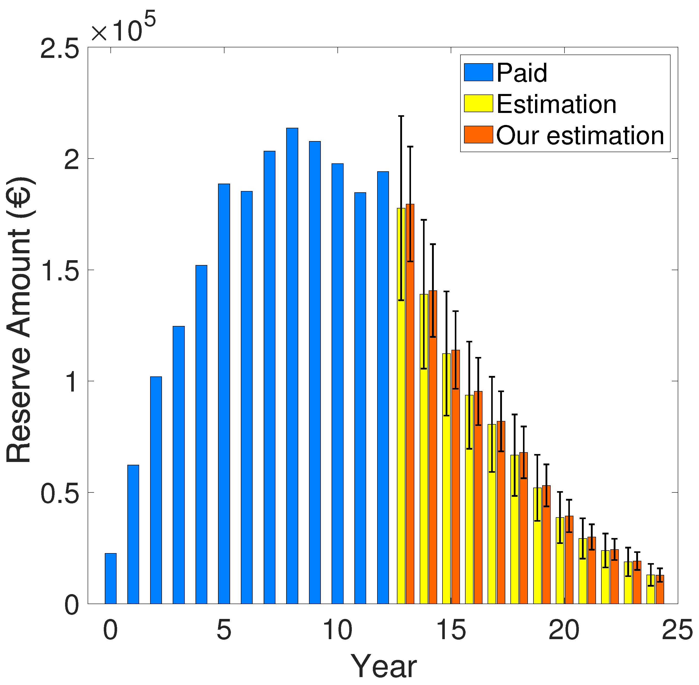
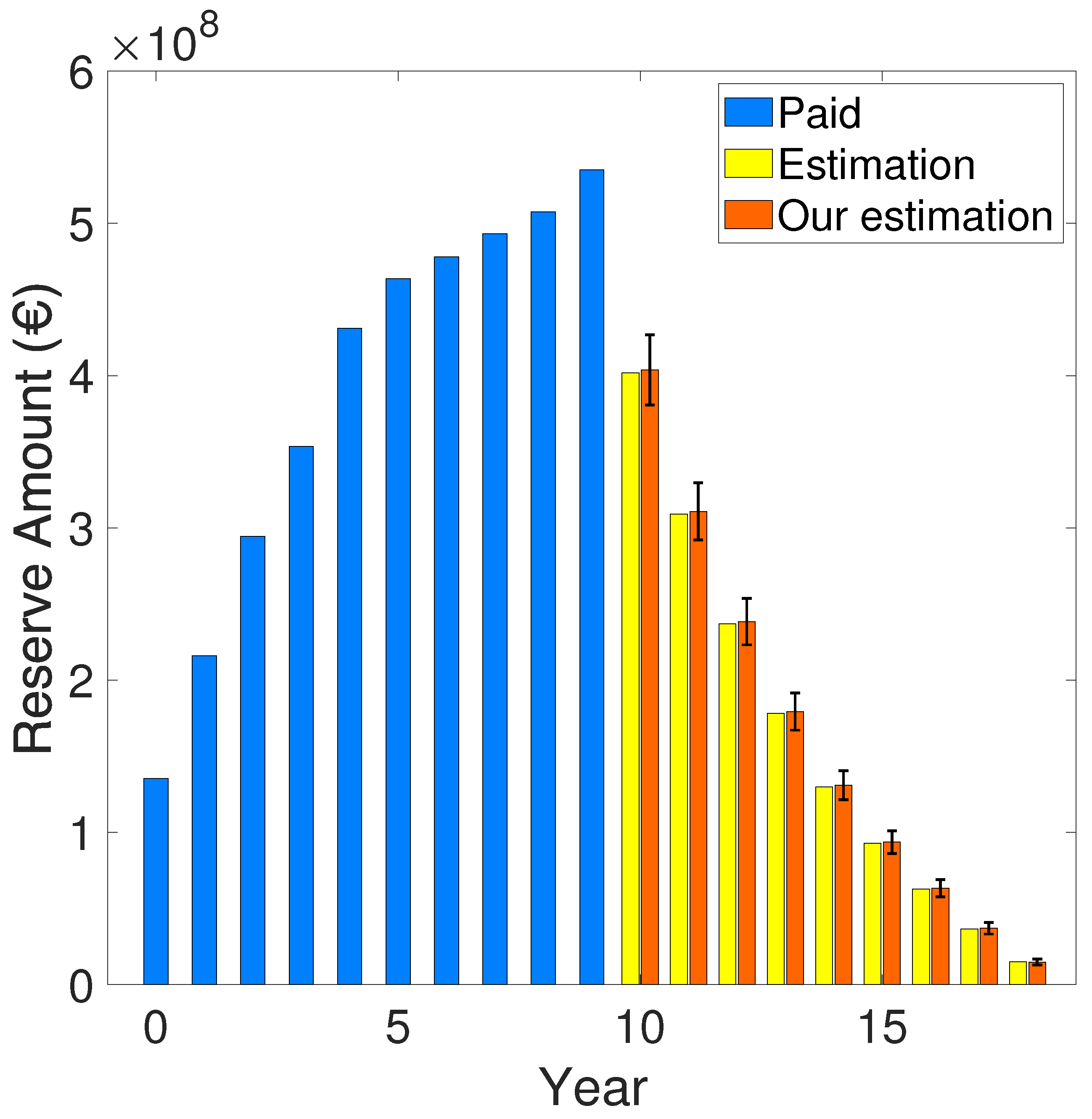
The data-set used in the work of [22] presents a Run-Off triangle filled in the context of “RC cars”, which is a well-known benchmark to test and validate the new methodology and theory of forecasting model especially in claims reserve estimation due to their small data dispersion and homogeneity. The authors applied the method previously described, using both residues defined in Section 2.4 to reproduce the results of [22]. The developed stochastic approach has been applied to predict the claims reserve

R^{(t)}

for the generic budget year (t) using equation 58, and it has been compared with the one provided by the optimization of [22]. The results concerning the predicted claims reserve

R^{(t)}

for the generic budget year (t), are depicted in the following two figures. Figure 1 shows the paid amount (

R^{(t)}

in the equation 60) and the predicted claims reserve (

R^{(t)}

in equation 58) relative to the comparison between [22] and our methodology using the residue defined in equation 46. Figure 2 shows the paid amount and the predicted claims reserve relative to the comparison between [22] and our methodology using the residue defined in equation 47. The obtained numerical results for the predicted claims reserve for a specific budget year are summarized in Table 3.

The obtained numerical results comprehending the value of the

S (β^{*})

function, the corresponding dispersion parameter (

ϕ

), and the total predicted total claims reserve amount

R_{t o t}

are summarized in Table 4.

It is essential to mention that in both cases, i.e. in the estimation provided by the authors, the convergence of the GN algorithm is improved because the authors used the GA to calculate the initial guess of parameters

β

(see Section 2.5). In contrast, concerning the work of [22], the algorithm’s convergence might converge to a local minimum without starting with an appropriate initial guess, leading to an increase in the errors associated with the

β

parameters. Additionally, it is important to mention that, the computed values of the

S (β^{*})

function, the dispersion parameter (

ϕ

), and the total predicted claims reserve amount

R_{t o t}

for the work of [22] have been obtained using the

β^{*}

parameters resulted by their calculation. The errors on the predicted claims reserve for the specific year

R^{(t)}

have been calculated using the error propagation by summing the errors relative to every single cell of the predicted values (

Δ μ_{i}

- see equation 57). The error propagation theory has been applied to calculate the entire predicted claims reserve

R_{t o t}

. Furthermore, using the two different definitions of the residues, the estimation of the claims reserve performed by the authors provides confidence intervals slightly lower than the ones provided by [22]. Even if the difference between the two residues is negligible for this case, the high dispersion and data aleatory in other contexts, such as healthcare, might produce more prominent confidence intervals.

3.2. Comparison with [23]

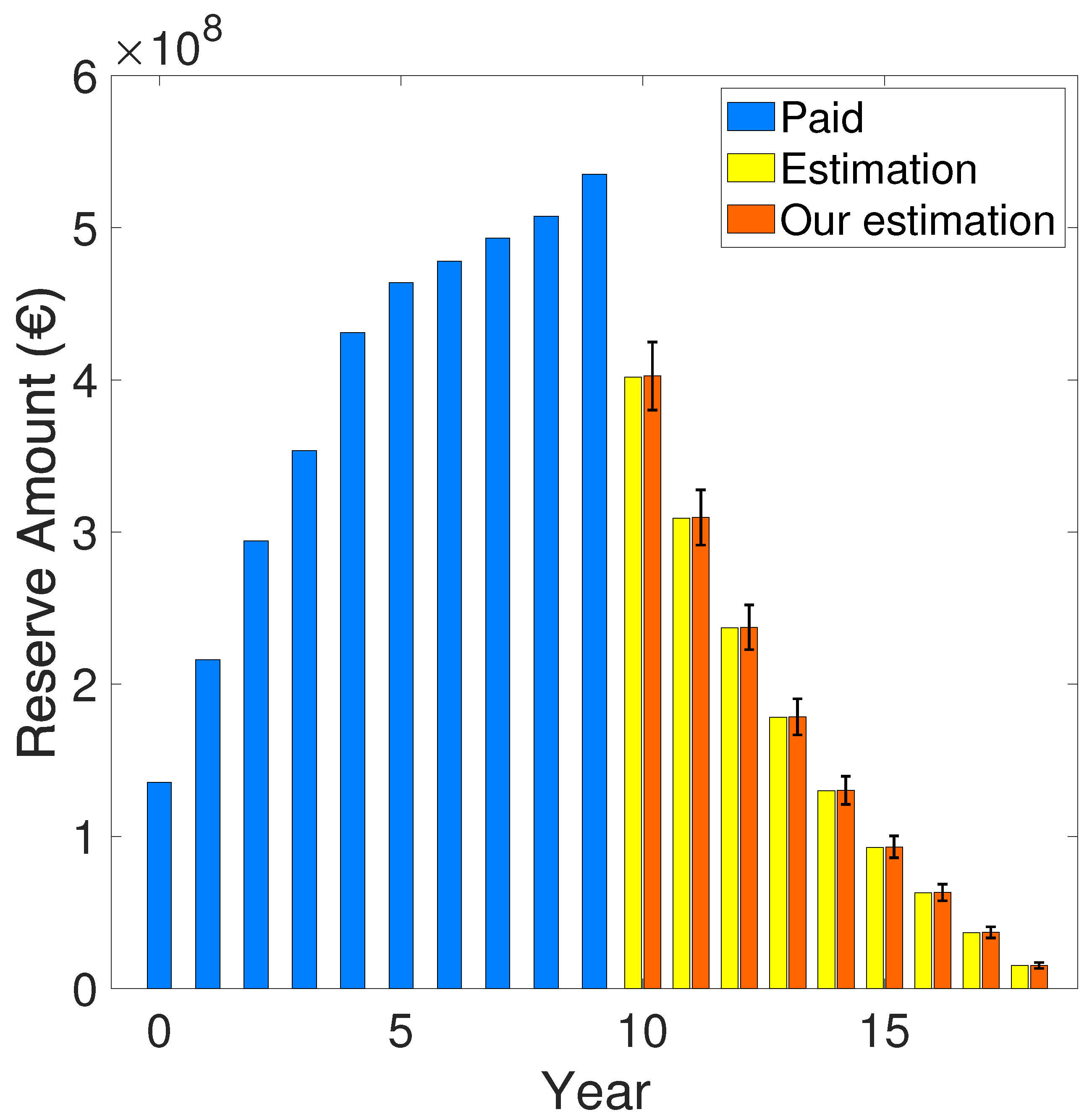
In this Section, the authors performed the validation approach of Section 3.1 with the Run-Off triangle presented in the work of [23]. In this case, [23] did not compute the errors associated with their stochastic model because they focused on developing a robustification of the CL method. However, the possibility to reproduce and improve the results presented in the work of [23] represents an excellent manner to validate further the methodology described in this paper since they present a low disperse data-set. Following the identical procedure of Section 3.1, the authors show the results of the developed stochastic model using the two definitions of the residues in equations 46 and 47, respectively. The results concerning the predicted claims reserve

R^{(t)}

for the generic budget year (t), are depicted in the following two figures. Figure 3 shows the paid amount (

R^{(t)}

in the equation 60) and the predicted claims reserve (

R^{(t)}

in equation 58) relative to the comparison between [22] and our methodology using the residue defined in equation 46. Figure 4 shows the paid amount and the predicted claims reserve relative to the comparison between [23] and our methodology using the residue defined in equation 47. The obtained numerical results for the predicted claims reserve for a specific budget year are summarized in Table 5.

In this case, the authors provided the results concerning the value of the

S (β^{*})

function, the corresponding dispersion parameter (

ϕ

), and the claims reserve amount applied to the Run-Off in the work of [23]. The results are shown in Table 6. Since [23] did not provide the errors associated with their stochastic model, the authors are unable to perform a consistent comparison with the work of literature, but they only provide the claims reserve amount coming from a robustification of the CL method.

Even in this case, both cases in the estimation provided by the authors, the convergence of the GN algorithm is improved because the authors used the GA to calculate the initial guess of parameters

β

(see Section 2.5). Furthermore, using the two different definitions of the residues, the calculation performed by the authors provides confidence intervals for the claims reserve that include the values calculated by [23] using a completely different approach.

4. The health care study: the case of claims in the Tuscany Region

The main objective is to apply the developed methodology to predict the total claims reserve to be set aside by the insurance agency. Specifically, the authors worked on the health insurance context of claims concerning the Tuscany Region in Italy to provide results for the reserve amount required by the region to manage the yearly balance finance system in healthcare. It is essential to notice that the authors carried on the stochastic analysis on claims reserve employing the two definitions of residues described in Section 2.4, providing accordingly to the SoA a new methodology to deal with claims reserve and the corresponding errors. The novelty and the contribution of our research take credit not only from the improvements compared with the SoA but also in the healthcare context. In order to test our methodology in the healthcare insurance system of the Tuscany Region, the author proceeded in the following manner. Firstly, the authors performed a preliminary analysis of the available healthcare insurance data-set to understand the useful information that can be retrieved in order to compile the Run-Off triangle. Secondly, the authors compared the CL methodology with the developed stochastic approach. The CL is a deterministic method used in different contexts to compute the one-year reserve. Subsequently, the authors reproduced the deterministic result with the developed stochastic model. Finally, the authors found the optimal parameters of the ODP to perform prediction for the entire claims reserve to provide an outcome to the region, which could be used in the management, together with the corresponding confidence intervals.

4.1. Preliminary analysis

The authors worked with the Centro Gestione Rischio Clinico of the Tuscany Region database concerning the healthcare claims reported from 2010 and 2021. In this Section, the authors performed a preliminary analysis retrieving the following information:

Time evolution of the paid claims;
Single payment for years of the specific claim;
Total paid amounts.

Starting from the provided dataset, it is possible to compile the following Run-Off triangle, which is the base of our research (Section 2.1). The rows of the Run-Off triangle are filled with the incurred years (i.e. from 2010 to 2021). The columns of the Run-Off triangle are filled with the progression of the payments towards the years. In this way, each cell represents the delayed payment with respect to the corresponding incurred year. Following the Run-Off triangle of the health insurance claims for the Tuscany Region is shown Table 7:

The variable

y_{i, j}

in Table 7 identifies the paid amount of the payment for claims that have been incurred in the

i^{t h}

year with a delay occurred in the

j^{t h}

year. As previously discussed, authors present the deterministic analysis of the Run-Off triangle shown in Table 7 employing the well-known CL approach. This analysis represents the benchmark of our research, as it will be compared with the proposed stochastic method by the authors in the following Sections.

4.2. Chain Ladder Results

The CL method provides a mechanism to forecast future loss development trends based on historical patterns. It offers a deterministic perspective on reserving losses for the subsequent year. This Section outlines the results of the CL method applied to the previous Run-Off triangle. The approach has been comprehensively explained in the referenced studies [22,26]. The results obtained by applying the CL method to the health insurance of the Tuscany Region are summarised in Table 8.

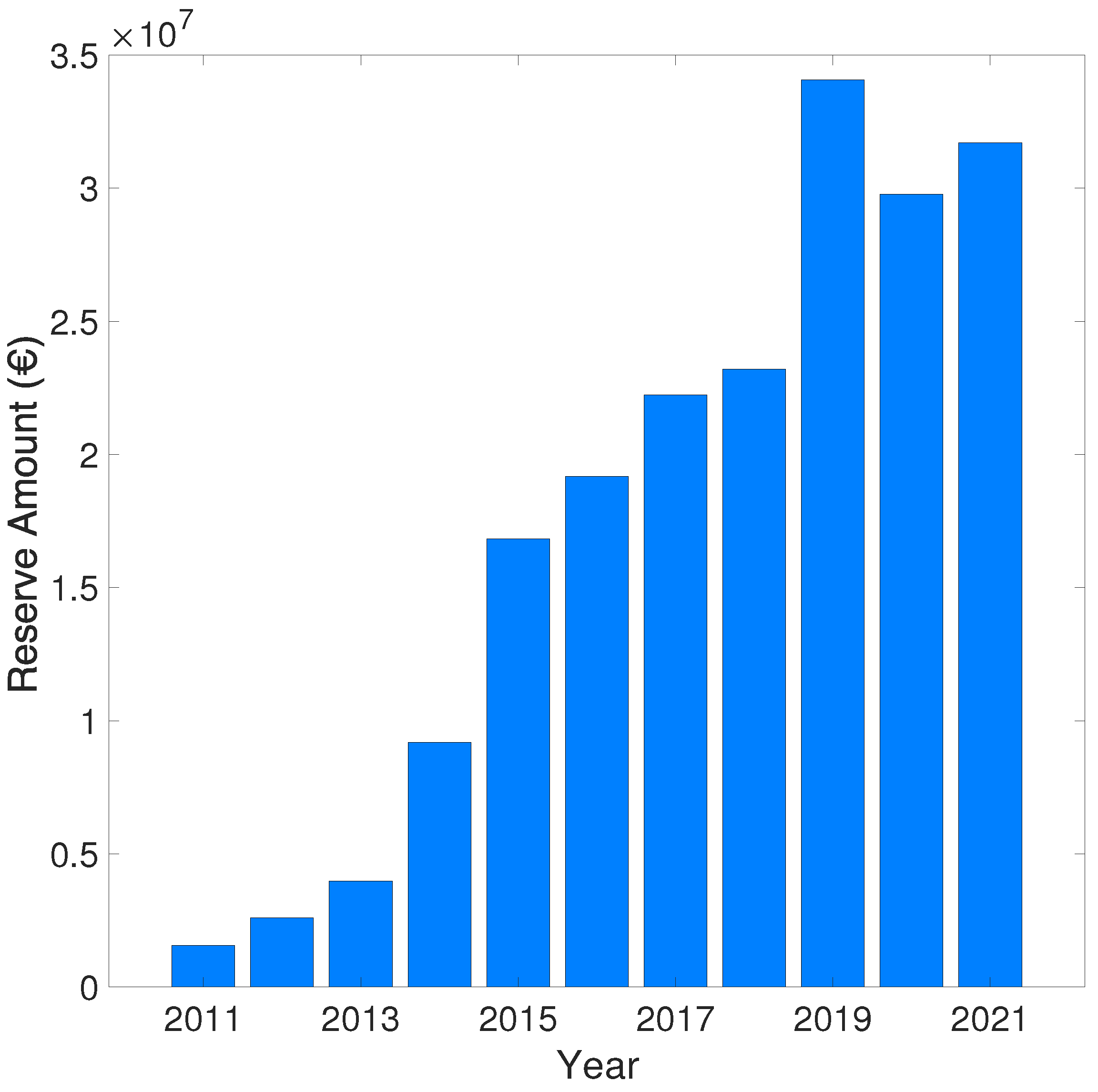
In this case, the predicted claims reserve amount

R^{(t)}

appearing in Table 8 has been calculated using equation 4, while the total predicted claims reserve amount for the Tuscany Region in the incurred years 2010-2021 is roughly:

R_{t o t} = 194.32 \times 10^{6} €

. Figure 5 shows the predicted claims reserve amount

R^{(t)}

for every single incurred year (2010-2021) employing the CL methodology. Despite the simplicity of the CL method, several issues make it unable to perform our analysis. Indeed it cannot provide and predict changes in the model, and it can only predict the one-year estimate of the claims reserve. Therefore, a stochastic method is needed to provide more complete results for claims reserve predictions and confidence intervals. In the following Section 4.3, the authors present the developed stochastic approach with the corresponding numerical results compared to the CL approach.

4.3. Stochastic Approach Results

The results obtained by applying the developed stochastic approach to estimate the claims reserve for the Tuscany Region are presented in this Section. In this Section, the values and the corresponding errors of the parameters (

β^{*}

) resulting from the developed stochastic approach are shown for the Tuscany Region insurance claims using both residue defined in equations 46 and 47. The procedure described in Section 2.4 and Section 2.5 has been applied to calculate the

β^{*}

parameters needed to compile the Run-Off triangle. The GA has been applied firstly to glimpse a good initial guess of

β

parameters, and subsequently, the GN algorithm has been applied to reach the stationary point

β^{*}

. The following Table 9 provides the results of the entire estimation for the

β

parameters and the corresponding errors.

At this step, it is possible to compute the expectation value

μ_{i, j}

for each insurance year (2010-2021) and fulfil the Run-Off triangle as shown in Section 3. The following Table 10 and Table 11 represent the Run-Off triangles compiled with the estimation provided by the entire procedure described in Section 2.4 and Section 2.6.

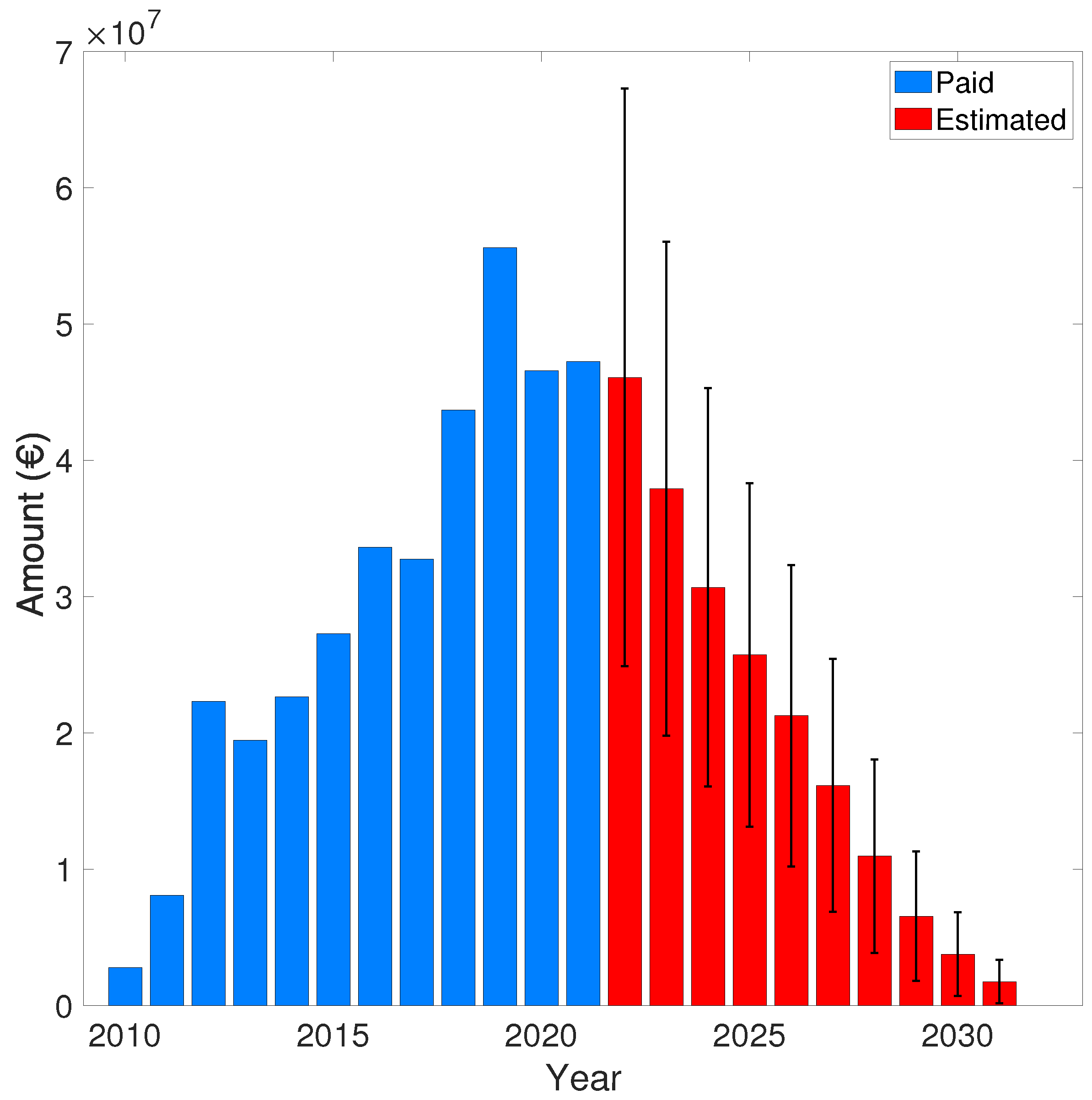
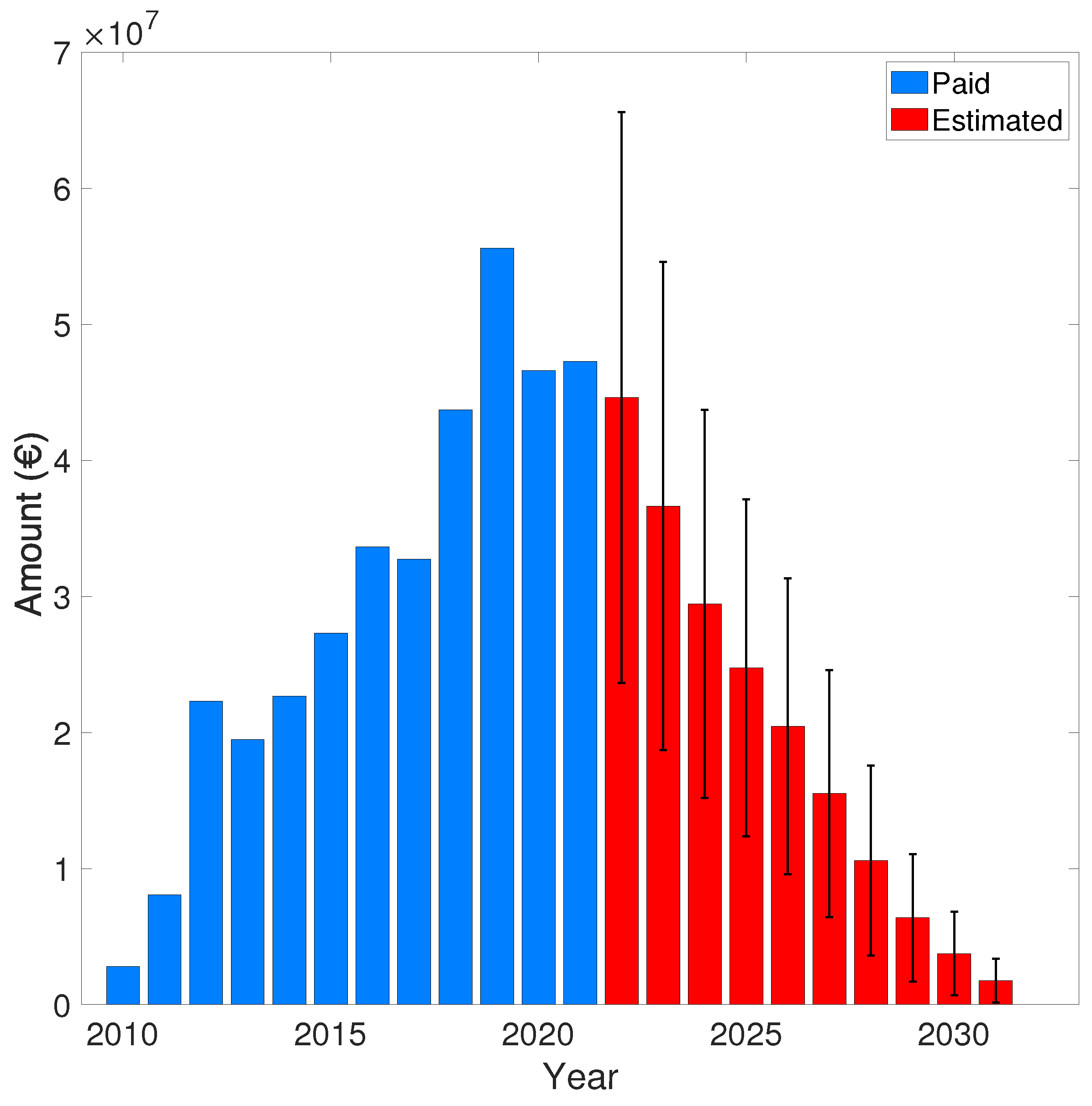
Given the expectation values

μ_{i, j}

shown in the previous Table 10 and Table 11, the authors provided the following figures representing the paid amount and the predicted claims reserve

R^{(t)}

for the generic budget year (t) from 2010 to 2031 in the Tuscany Region.

Referring to the previous Figure 6 and Figure 7, the Table 12 presents the complete set of values concerning the paid amount and the predicted claims reserve

R^{(t)}

for the generic budget year (t) from 2010 to 2031 in the Tuscany Region.

In Table 13, the authors provided the values of the KPI resulting from the estimation of the total reserve to be set aside for the Tuscany Region insurance claims. Specifically, the value of the

S (β^{*})

function, the corresponding dispersion parameter (

ϕ

), the predicted claims reserve amount for the 2021 incurred year

R^{(2021)}

, and the total predicted claims reserve

R_{t o t}

computed using equation 59.

The results in Table 13 illustrate the predictive accuracy of the stochastic model developed by the authors, which was previously validated as described in Section 3. It is important to note that the absolute errors on the predicted claims reserve are considerable off an interval of acceptability (i.e. the estimated errors are roughly 50 % of the predicted values for the claims reserve). The reason is due to the high data dispersion that the stochastic model is unable to overcome. Nevertheless, compared to the current SoA, the analysis conducted by the authors for the healthcare sector is entirely satisfactory, as it represents a notable initial approach to estimating the claims reserve in a highly heterogeneous and mutable context.

5. Conclusion

In this work, the authors contributed to creating a robust protocol to deal with claims reserve in the healthcare system context. Even if the SoA already presented a well-defined approach for claims reserve in the healthcare system, the wide variability, peculiarity, and aleatory made necessary reformulation and subsequent improvements of the stochastic methodology usually adopted. Therefore, the authors contributed to the SoA, improving the management of claims reserve in such a way that is easy to reproduce by the institutions which are the final users (i.e. the Tuscany Region) without increasing computational costs. Possible developments of the method concern the possibility of expanding the Run-Off tables, predicting the durability of the entire claims life, and defining a method to improve the error estimations also for highly dispersed databases such as the one of the healthcare context as treated in this work. Furthermore, it is necessary to create a unique protocol for data management to improve the quality and accessibility of the data and develop a robust analysis of the incurred velocity.

Acknowledgments

The authors sincerely thank the Tuscany Region and, particularly Dr. Federico Gelli and Dr. Michela Maielli; the Centro Gestione Rischio Clinico, and in particular Dr. Elisa Flore, Dr. Francesca Guerrini, and Dr. Pasquale Macrì; Prof. Nino Savelli, and Prof. Gian Paolo Clemente for the important feedback and support and Prof. Chiara Seghieri from MeS laboratory of Sant’Anna School for Advanced Studies. The research project developed in this paper is funded by Tuscany Region.

Conflicts of Interest

The authors declare that there is no conflict of interest regarding the publication of this article.

References

Institute of Medicine (U.S.) Committee on Quality of Health Care in America. To Err is Human - Building a safer health system.
Delivering quality health services: a global imperative for universal health coverage. OECD, World Health Organization & World Bank Group. OECD Publishing.
2021. State of Health in the EU: Italy. OECD, European Commission & European Observatory on Health Systems and Policies. OECD Publishing.
Conn, Andrew, Nicholas Gould, and Philippe Toint. 1991, 04. A globally convergent augmented lagrangian algorithm for optimization with general constraints and simple bounds. SIAM Journal on Numerical Analysis 28. [CrossRef]
Conn, Andrew, Nicholas Gould, and Philippe Toint. 1997. A globally convergent augmented lagrangian barrier algorithm for optimization with general inequality constraints and simple bounds. Mathematics of Computation 66, 261–268. [CrossRef]
D. Mushinski; S. Zahran; A. Frazier. 2022. Physician behaviour, malpractice risk and defensive medicine: an investigation of cesarean deliveries. Health Economics, Policy and Law. [CrossRef]
England, Peter and Richard Verrall. 1999. Analytic and bootstrap estimates of prediction errors in claims reserving. Insurance: Mathematics and Economics 25(3), 281–293. [CrossRef]
England, P D and R J Verrall. 2002. Stochastic claims reserving in general insurance. British Actuarial Journal 8, 443–544.
Fletcher, R. 2000. Practical Methods of Optimization, 2nd Edition. Wiley. [CrossRef]
Goldberg, David E. 1989. Genetic Algorithms in Search, Optimization and Machine Learning. Addison-Wesley Longman Publishing Co., Inc.
Hess, Klaus Th. and Klaus D Schmidt. 2002. A comparison of models for the chain–ladder method. Insurance: Mathematics and Economics 31, 351–364. [CrossRef]
Hindley, David. 2017, 10. Claims Reserving in General Insurance. Cambridge University Press. [CrossRef]
Jorge Nocedal and Stephen J. Wright. 2006. Numerical Optimization (2e ed.). New York, NY, USA: Springer.
Kendall, Maurice George and Alan Stuart. 1967. The Advanced Theory of Statistics (2 ed.). Hafner.
Larsen, Christian Roholte. 2007. An individual claims reserving model. ASTIN Bulletin 37(1), 113–132. [CrossRef]
Mascarenhas, Walter. 2013, 09. The divergence of the bfgs and gauss-newton methods. Mathematical Programming 147. [CrossRef]
Nelder, John Ashworth and Robert William Maclagan Wedderburn. 1972. Generalized Linear Model. Journal of the Royal Statistical Society: Series A 135, 370. [CrossRef]
Nuno, Grembi Veronica; Garoupa. 2013. Delays in medical malpractice litigation in civil law jurisdictions: Some evidence from the italian court of cassation. Health Economics, Policy and Law. 8(4), 423–452. [CrossRef]
Renshaw, A E and R J Verrall. 1998, 10. A stochastic model underlying the chain-ladder technique. British Actuarial Journal 4, 903–923. [CrossRef]
Schmidt, Klaus D. 2006. Methods and models of loss reserving based on run-off triangles: A unifying survey. Casualty Actuarial Society Forum 2006, 269–317.
Schmidt, Klaus D. 2012. Loss prediction based on run-off triangles. AStA Advances in Statistical Analysis 96, 265 – 310. [CrossRef]
Strascia, Stefano Cavastracci and Agostino Tripodi. 2018. Overdispersed-poisson model in claims reserving: Closed tool for one-year volatility in glm framework. Risks 6. [CrossRef]
Verdonck, Tim, Martine Van Wouwe, and Jan Dhaene. 2009. A robustification of the chain-ladder method. North American Actuarial Journal 13, 280 – 298. [CrossRef]
Veronica, Bertoli Paola; Grembi. 2018. Courts, scheduled damages, and medical malpractice insurance. Empirical Economics 55, 831–854. [CrossRef]
Verrall, R.J. 2000. An investigation into stochastic claims reserving models and the chain-ladder technique. Insurance: Mathematics and Economics 26(1), 91–99. [CrossRef]
Verrall, R J. 1991. Chain ladder and maximum likelihood. Journal of the Institute of Actuaries (1886-1994) 118, 489–499.
Wedderburn, R W M. 1974. Quasi-likelihood functions, generalized linear models, and the gauss-newton method. Biometrika 61, 439 – 447. [CrossRef]
Wedderburn, R W M. 1976. On the existence and uniqueness of the maximum likelihood estimates for certain generalized linear models. Biometrika 63, 27 – 32. [CrossRef]

1	Data in the present paper are smoothed for policy and legal motivations.
2	A nuisance parameter is any unspecified parameter necessary to ensure that the model describes the system adequately. In our case, it represents the dispersion of the measured data.

Figure 1. Computed reserve amount between our approach and the one provided by [22], using the residue defined in equation 46 for the GN algorithm. The "blue" bars indicate the paid amounts computed using equation 60, while the "yellow" and the "orange" error-bars indicate the predicted claims reserve computed using equation 58 for [22] and our work, respectively.

Figure 2. Computed reserve amount between our approach and the one provided by [22], using the residue defined in equation 47 for the GN algorithm. The "blue" bars indicate the paid amounts computed using equation 60, while the "yellow" and the "orange" error-bars indicate the predicted claims reserve computed using equation 58 for [22] and our work, respectively.

Figure 3. Computed reserve amount between our approach and the one provided by [23], using the residue defined in equation 46 for the GN algorithm. The "blue" bars indicate the paid amounts computed using equation 60, while the "yellow" and the "orange" error-bars indicate the predicted claims reserve computed using equation 58 for [23] and our work, respectively.

Figure 4. Computed reserve amount between our approach and the one provided by [23], using the residue defined in equation 47 for the GN algorithm. The "blue" bars indicate the paid amounts computed using equation 60, while the "yellow" and the "orange" error-bars indicate the predicted claims reserve computed using equation 58 for [23] and our work, respectively.

Figure 5. Predicted claims reserve amount

R^{(t)}

for every single incurred year (2010-2021) using the CL method.

Figure 5. Predicted claims reserve amount

R^{(t)}

for every single incurred year (2010-2021) using the CL method.

Figure 6. Paid amount and the predicted claims reserve

R^{(t)}

for the generic budget year (t) from 2010 to 2031 in the Tuscany Region computed using the Residue defined in equation 46.

Figure 6. Paid amount and the predicted claims reserve

R^{(t)}

for the generic budget year (t) from 2010 to 2031 in the Tuscany Region computed using the Residue defined in equation 46.

Figure 7. Paid amount and the predicted claims reserve

R^{(t)}

for the generic budget year (t) from 2010 to 2031 in the Tuscany Region computed using the Residue defined in equation 47.

Figure 7. Paid amount and the predicted claims reserve

R^{(t)}

for the generic budget year (t) from 2010 to 2031 in the Tuscany Region computed using the Residue defined in equation 47.

Table 1. Example of Run-Off triangle. The variable

y_{i, j}

indicates the paid amount relative to a claim that has occurred in the

i^{t h}

incurred year where the effective payment has been delayed in the

j^{t h}

year.

Table 1. Example of Run-Off triangle. The variable

y_{i, j}

indicates the paid amount relative to a claim that has occurred in the

i^{t h}

incurred year where the effective payment has been delayed in the

j^{t h}

year.

$i / j$	0	1	…	j	…	$J - 1$	J
1	$y_{1, 0}$	$y_{1, 1}$	…	$y_{1, j}$	…	$y_{1, J - 1}$	$y_{1, J}$
2	$y_{2, 0}$	$y_{2, 1}$	…	$y_{2, j}$	…	$y_{2, J - 1}$
...	...	...		...
i	$y_{i, 0}$	$y_{i, 1}$	…	$y_{i, j}$
...	...	...
$I - 1$	$y_{I - 1, 0}$	$y_{I - 1, 1}$
I	$y_{I, 0}$

Table 2. Complete set of expectation values

μ_{i, j}

computed using the developed stochastic model.

Table 2. Complete set of expectation values

μ_{i, j}

computed using the developed stochastic model.

$i / j$	0	1	…	j	…	$J - 1$	J
1	$μ_{1, 0}$	$μ_{1, 1}$	…	$μ_{1, j}$	…	$μ_{1, J - 1}$	$μ_{1, J}$
2	$μ_{2, 0}$	$μ_{2, 1}$	…	$μ_{2, j}$	…	$μ_{2, J - 1}$	$μ_{2, J}$
...	...	...		...		...	...
i	$μ_{i, 0}$	$μ_{i, 1}$	…	$μ_{i, j}$	…	$μ_{i, J - 1}$	$μ_{i, J}$
...	...	...		...		...	...
$I - 1$	$μ_{I - 1, 0}$	$μ_{I - 1, 1}$	…	$μ_{I - 1, j}$	…	$μ_{I - 1, J - 1}$	$μ_{I - 1, J}$
I	$μ_{I, 0}$	$μ_{I, 1}$	…	$μ_{I, j}$	…	$μ_{I, J - 1}$	$μ_{I, J}$

Table 3. Comparison between our developed methodology and the work of [22] in predicting claims reserve

R^{(t)}

for the specific budget year

t \in [I + 1, I + J]

for the two residues.

Table 3. Comparison between our developed methodology and the work of [22] in predicting claims reserve

R^{(t)}

for the specific budget year

t \in [I + 1, I + J]

for the two residues.

Budget year (t)	Paid (10³ €) Literature	$R^{(t)}$ (10³ €) Literature	$R^{(t)}$ (10³ €) Residue (Eq. 46)	$R^{(t)}$ (10³ €) Residue (Eq. 47)
0	22.60	-	22.60 ± 1.43	22.60 ± 1.43
1	62.32	-	62.32 ± 5.70	62.32 ± 5.65
2	101.93	-	101.93 ± 9.25	101.93 ± 9.03
3	124.59	-	124.59 ± 12.12	124.59 ± 11.57
4	152.04	-	152.04 ± 14.82	152.04 ± 13.85
5	188.65	-	188.65 ± 17.33	188.65 ± 16.03
6	185.31	-	185.31 ± 19.72	185.31 ± 18.45
7	203.38	-	203.38 ± 21.77	203.38 ± 20.40
8	213.67	-	213.67 ± 23.03	213.67 ± 21.37
9	207.65	-	207.65 ± 23.39	207.65 ± 21.63
10	197.67	-	197.67 ± 23.64	197.67 ± 21.84
11	184.68	-	184.68 ± 24.99	184.68 ± 23.10
12	194.08	-	194.08 ± 29.10	194.08 ± 27.00
13	-	177.71 ± 41.39	183.87 ± 27.96	179.53 ± 25.78
14	-	139.04 ± 33.41	146.17 ± 22.90	140.69 ± 20.80
15	-	112.39 ± 27.91	119.75 ± 19.38	113.99 ± 17.43
16	-	93.69 ± 24.06	101.15 ± 16.98	95.37 ± 15.13
17	-	80.55 ± 21.36	85.66 ± 14.89	81.93 ± 13.48
18	-	66.73 ± 18.32	71.52 ± 12.90	67.97 ± 11.61
19	-	52.05 ± 14.84	57.26 ± 10.72	53.14 ± 9.43
20	-	38.71 ± 11.50	42.30 ± 8.21	39.44 ± 7.26
21	-	29.33 ± 9.05	32.14 ± 6.44	29.97 ± 5.71
22	-	23.89 ± 7.62	26.14 ± 5.41	24.38 ± 4.78
23	-	18.78 ± 6.39	20.36 ± 4.50	19.19 ± 4.00
24	-	12.95 ± 4.93	13.69 ± 3.40	12.85 ± 3.01

Table 4. Comparison between the work of [22] and our proposed methodology concerning the

S (β^{*})

function (equation 22), the dispersion parameter

ϕ

(equation 16), and the total predicted claims reserve amount

R_{t o t}

(equation 59) for both residues (Section 2.4).

Table 4. Comparison between the work of [22] and our proposed methodology concerning the

S (β^{*})

function (equation 22), the dispersion parameter

ϕ

(equation 16), and the total predicted claims reserve amount

R_{t o t}

(equation 59) for both residues (Section 2.4).

Residue (Eq. 46)	Reference	$S (β^{*})$	$ϕ$	$R_{t o t}$ ( $10^{5}$ €)
	[22]	$3.65 \times 10^{5}$	$4.11 \times 10^{2}$	8.46 ± 2.20
	Our work	$3.00 \times 10^{5}$	$4.53 \times 10^{2}$	9.00 ± 1.54
Residue (Eq. 47)	Reference	$S (β^{*})$	$ϕ$	$R_{t o t}$ ( $10^{5}$ €)
	[22]	$2.71 \times 10^{4}$	$4.11 \times 10^{2}$	8.46 ± 2.20
	Our work	$2.68 \times 10^{4}$	$4.06 \times 10^{2}$	8.58 ± 1.38

Table 5. Comparison between our developed methodology and the work of [23] in predicting claims reserve

R^{(t)}

for the specific budget year

t \in [I + 1, I + J]

for the two residues.

Table 5. Comparison between our developed methodology and the work of [23] in predicting claims reserve

R^{(t)}

for the specific budget year

t \in [I + 1, I + J]

for the two residues.

Budget year (t)	Paid (10⁶ €) Literature	$R^{(t)}$ (10⁶ €) Literature	$R^{(t)}$ (10⁶ €) Residue (Eq. 46)	$R^{(t)}$ (10⁶ €) Residue (Eq. 47)
0	135.34	-	135.34 ± 3.05	135.34 ± 2.92
1	216.03	-	216.03 ± 7.56	216.03 ± 7.38
2	294.31	-	294.31 ± 11.12	294.31 ± 10.84
3	353.38	-	353.38 ± 14.22	353.38 ± 13.84
4	431.01	-	431.01 ± 17.14	431.01 ± 16.69
5	463.80	-	463.80 ± 19.19	463.80 ± 18.65
6	478.03	-	478.03 ± 20.99	478.03 ± 20.33
7	493.10	-	493.10 ± 22.89	493.10 ± 22.20
8	507.59	-	507.59 ± 25.35	507.59 ± 24.53
9	535.26	-	535.26 ± 28.75	535.26 ± 27.84
10	-	401.96	403.74 ± 23.07	402.54 ± 22.35
11	-	309.07	310.82 ± 18.74	309.57 ± 18.13
12	-	236.98	238.43 ± 15.25	237.42 ± 14.75
13	-	178.16	179.39 ± 12.26	178.56 ± 11.86
14	-	129.86	131.02 ± 9.57	130.23 ± 9.24
15	-	92.78	93.62 ± 7.45	93.08 ± 7.19
16	-	62.85	63.36 ± 5.61	63.08 ± 5.43
17	-	36.63	37.03 ± 3.82	36.83 ± 3.69
18	-	15.12	14.87 ± 1.93	15.11 ± 1.90

Table 6. Comparison between the work of [23] and our proposed methodology concerning the

S (β^{*})

function (equation 22), the dispersion parameter

ϕ

(equation 16), and the total predicted claims reserve amount

R_{t o t}

(equation 59) for both residues (Section 2.4).

Table 6. Comparison between the work of [23] and our proposed methodology concerning the

S (β^{*})

function (equation 22), the dispersion parameter

ϕ

(equation 16), and the total predicted claims reserve amount

R_{t o t}

(equation 59) for both residues (Section 2.4).

Residue (Eq. 46)	Reference	$S (β^{*})$	$ϕ$	$R_{t o t}$ ( $10^{9}$ €)
	[23]	-	-	1.46
	Our work	$8.57 \times 10^{6}$	$2.02 \times 10^{5}$	1.47 ± 0.09
Residue (Eq. 47)	Reference	$S (β^{*})$	$ϕ$	$R_{t o t}$ ( $10^{9}$ €)
	[23]	-	-	1.46
	Our work	$6.81 \times 10^{6}$	$1.89 \times 10^{5}$	1.47 ± 0.09

Table 7. Paid amount of the Run-Off triangle for health insurance claims for the Tuscany Region from 2010 to 2021 (10⁶ €).

$y_{i, j}$	0	1	2	3	4	5	6	7	8	9	10	11
2010	2.80	5.94	10.1	5.00	4.06	4.28	2.74	1.98	2.64	1.06	1.20	1.27
2011	2.13	11.3	6.15	1.79	2.82	4.29	5.26	7.76	4.91	3.35	1.43
2012	0.95	7.61	7.19	3.25	4.77	3.08	5.03	5.65	3.64	1.74
2013	0.72	8.66	5.68	1.63	3.44	4.06	4.89	3.95	2.50
2014	0.97	9.76	7.67	6.49	4.07	5.66	4.41	3.90
2015	1.50	11.4	7.17	3.95	6.52	5.76	7.87
2016	1.15	5.14	9.14	9.74	3.33	2.95
2017	0.19	6.96	8.92	5.77	3.63
2018	0.10	5.90	9.36	3.68
2019	2.35	5.55	10.9
2020	0.27	6.57
2021	0.81

Table 8. Predicted claims reserve amount

R^{(t)}

for every single incurred year

(t)

using the CL method.

Table 8. Predicted claims reserve amount

R^{(t)}

for every single incurred year

(t)

using the CL method.

t	$R^{(t)}$ (€)
2011	$1.56 \times 10^{6}$
2012	$2.59 \times 10^{6}$
2013	$3.97 \times 10^{6}$
2014	$9.19 \times 10^{6}$
2015	$16.83 \times 10^{6}$
2016	$19.17 \times 10^{6}$
2017	$22.24 \times 10^{6}$
2018	$23.21 \times 10^{6}$
2019	$34.07 \times 10^{6}$
2020	$29.78 \times 10^{6}$
2021	$31.70 \times 10^{6}$

Table 9. Estimated parameters (

β^{*}

) using both residues defined in equations 46 and 47.

Table 9. Estimated parameters (

β^{*}

) using both residues defined in equations 46 and 47.

Residue (Eq. 46)			Residue (Eq. 47)
Variable	Value	Error	Variable	Value	Error
c	14.183	0.221	c	14.109	0.226
$a_{1}$	0.175	0.155	$a_{1}$	0.197	0.156
$a_{2}$	-0.022	0.164	$a_{2}$	0.002	0.165
$a_{3}$	-0.103	0.170	$a_{3}$	-0.114	0.172
$a_{4}$	0.126	0.165	$a_{4}$	0.140	0.166
$a_{5}$	0.286	0.165	$a_{5}$	0.313	0.166
$a_{6}$	0.191	0.177	$a_{6}$	0.178	0.179
$a_{7}$	0.048	0.193	$a_{7}$	0.055	0.195
$a_{8}$	-0.011	0.209	$a_{8}$	-0.047	0.213
$a_{9}$	0.164	0.217	$a_{9}$	0.190	0.216
$a_{10}$	-0.158	0.313	$a_{10}$	-0.191	0.320
$a_{11}$	-0.572	0.889	$a_{11}$	-0.498	0.883
$b_{1}$	1.655	0.205	$b_{1}$	1.701	0.210
$b_{2}$	1.682	0.207	$b_{2}$	1.740	0.212
$b_{3}$	1.244	0.220	$b_{3}$	1.247	0.226
$b_{4}$	0.994	0.233	$b_{4}$	1.034	0.237
$b_{5}$	1.026	0.237	$b_{5}$	1.075	0.241
$b_{6}$	1.216	0.238	$b_{6}$	1.248	0.242
$b_{7}$	1.239	0.248	$b_{7}$	1.252	0.253
$b_{8}$	0.894	0.285	$b_{8}$	0.925	0.289
$b_{9}$	0.430	0.355	$b_{9}$	0.418	0.364
$b_{10}$	-0.186	0.522	$b_{10}$	-0.124	0.519
$b_{11}$	-0.125	0.724	$b_{11}$	-0.051	0.719

Table 10. Expectation values

μ_{i, j}

(10⁶ €) computed using the residue defined in equation 46.

Table 10. Expectation values

μ_{i, j}

(10⁶ €) computed using the residue defined in equation 46.

$μ_{i, j}$	0	1	2	3	4	5	6	7	8	9	10	11
2010	1.44	7.55	7.76	5.01	3.90	4.03	4.87	4.98	3.53	2.22	1.20	1.27
2011	1.72	9.00	9.24	5.97	4.65	4.80	5.80	5.94	4.20	2.64	1.43	1.52
2012	1.41	7.39	7.59	4.90	3.82	3.94	4.77	4.87	3.45	2.17	1.17	1.25
2013	1.30	6.81	7.00	4.52	3.52	3.63	4.39	4.49	3.18	2.00	1.08	1.15
2014	1.64	8.57	8.80	5.68	4.42	4.57	5.52	5.65	4.00	2.52	1.36	1.44
2015	1.92	10.1	10.3	6.67	5.19	5.36	6.48	6.63	4.70	2.95	1.60	1.70
2016	1.75	9.14	9.39	6.06	4.72	4.88	5.89	6.03	4.27	2.69	1.45	1.54
2017	1.52	7.93	8.14	5.26	4.09	4.23	5.11	5.23	3.70	2.33	1.26	1.34
2018	1.43	7.47	7.68	4.96	3.86	3.99	4.82	4.93	3.49	2.20	1.19	1.26
2019	1.70	8.90	9.14	5.90	4.60	4.75	5.74	5.87	4.16	2.62	1.41	1.50
2020	1.23	6.45	6.63	4.28	3.33	3.44	4.16	4.25	3.01	1.90	1.02	1.09
2021	0.81	4.26	4.38	2.83	2.20	2.27	2.75	2.81	1.99	1.25	0.68	0.72

Table 11. Expectation values

μ_{i, j}

(10⁶ €) computed using the residue defined in equation 47.

Table 11. Expectation values

μ_{i, j}

(10⁶ €) computed using the residue defined in equation 47.

$μ_{i, j}$	0	1	2	3	4	5	6	7	8	9	10	11
2010	1.34	7.35	7.64	4.67	3.77	3.93	4.67	4.69	3.38	2.04	1.18	1.27
2011	1.63	8.95	9.30	5.68	4.59	4.79	5.69	5.71	4.12	2.48	1.44	1.55
2012	1.34	7.36	7.66	4.68	3.78	3.94	4.68	4.70	3.39	2.04	1.19	1.28
2013	1.20	6.56	6.82	4.17	3.37	3.51	4.17	4.19	3.02	1.82	1.06	1.14
2014	1.54	8.45	8.79	5.37	4.34	4.52	5.37	5.40	3.89	2.34	1.36	1.47
2015	1.83	10.0	10.4	6.38	5.16	5.37	6.38	6.41	4.62	2.79	1.62	1.74
2016	1.60	8.78	9.13	5.58	4.51	4.70	5.58	5.61	4.04	2.43	1.42	1.52
2017	1.42	7.77	8.07	4.93	3.99	4.15	4.93	4.96	3.58	2.15	1.25	1.35
2018	1.28	7.01	7.29	4.45	3.60	3.75	4.46	4.48	3.23	1.94	1.13	1.22
2019	1.62	8.88	9.24	5.64	4.56	4.75	5.64	5.67	4.09	2.46	1.43	1.54
2020	1.11	6.07	6.31	3.86	3.12	3.25	3.86	3.88	2.79	1.68	0.98	1.05
2021	0.81	4.47	4.64	2.84	2.29	2.39	2.84	2.85	2.06	1.24	0.72	0.77

Table 12. Representation of the paid amount and predicted claims reserve

R^{(t)}

for the generic budget year provided with the two different definitions of the residues. From the budget year 2022 to 2031, the values of

R^{(t)}

are fully predicted.

Table 12. Representation of the paid amount and predicted claims reserve

R^{(t)}

for the generic budget year provided with the two different definitions of the residues. From the budget year 2022 to 2031, the values of

R^{(t)}

are fully predicted.

Budget year (t)	$R^{(t)}$ (10⁶ €) Paid Amount	$R^{(t)}$ (10⁶ €) Residue (Eq. 46)	$R^{(t)}$ (10⁶ €) Residue (Eq. 47)
2010	2.80	1.44 ± 0.32	1.34 ± 0.30
2011	8.08	9.27 ± 2.74	8.98 ± 2.71
2012	22.3	18.2 ± 5.79	17.9 ± 5.83
2013	19.5	22.9 ± 7.61	22.5 ± 7.63
2014	22.7	25.9 ± 8.76	25.2 ± 8.69
2015	27.3	31.1 ± 10.6	30.3 ± 10.5
2016	33.6	38.6 ± 13.3	37.8 ± 13.3
2017	32.8	44.9 ± 15.7	43.7 ± 15.5
2018	43.7	47.7 ± 17.0	46.2 ± 16.8
2019	55.6	48.8 ± 17.9	47.0 ± 17.5
2020	46.6	50.5 ± 19.1	48.7 ± 18.8
2021	47.3	50.5 ± 20.7	48.8 ± 20.3
2022	-	46.1 ± 21.2	44.6 ± 21.0
2023	-	37.9 ± 18.1	36.7 ± 17.9
2024	-	30.7 ± 14.6	29.4 ± 14.3
2025	-	25.7 ± 12.6	24.8 ± 12.4
2026	-	21.3 ± 11.1	20.5 ± 10.9
2027	-	16.2 ± 9.27	15.5 ± 9.08
2028	-	11.0 ± 7.10	10.6 ± 6.97
2029	-	6.56 ± 4.75	6.39 ± 4.69
2030	-	3.78 ± 3.08	3.76 ± 3.06
2031	-	1.76 ± 1.60	1.77 ± 1.62

Table 13. Results concerning the Tuscany Region analysis providing the values of the KPI such as

S (β^{*})

function (equation 22), the dispersion parameter

ϕ

(equation 16), the predicted claims reserve amount for the 2021 incurred year

R^{(2021)}

, and the total predicted claims reserve

R_{t o t}

Table 13. Results concerning the Tuscany Region analysis providing the values of the KPI such as

S (β^{*})

function (equation 22), the dispersion parameter

ϕ

(equation 16), the predicted claims reserve amount for the 2021 incurred year

R^{(2021)}

, and the total predicted claims reserve

R_{t o t}

	$S (β^{*})$	$ϕ$	$R^{(2021)}$ (10⁶ €)	$R_{t o t}$ (10⁶ €)
Measured	-	-	47.3	-
CL (Table 8)	-	-	31.7	-
Residue (Eq. 46)	6.78 × 10³	6.05 × 10⁵	50.5 ± 20.7	201 ± 103
Residue (Eq. 47)	3.27 × 10⁷	5.94 × 10⁵	48.8 ± 20.3	194 ± 102

Disclaimer/Publisher’s Note: The statements, opinions and data contained in all publications are solely those of the individual author(s) and contributor(s) and not of MDPI and/or the editor(s). MDPI and/or the editor(s) disclaim responsibility for any injury to people or property resulting from any ideas, methods, instructions or products referred to in the content.

© 2023 by the authors. Licensee MDPI, Basel, Switzerland. This article is an open access article distributed under the terms and conditions of the Creative Commons Attribution (CC BY) license (http://creativecommons.org/licenses/by/4.0/).

Copyright: This open access article is published under a Creative Commons CC BY 4.0 license, which permit the free download, distribution, and reuse, provided that the author and preprint are cited in any reuse.

MDPI Initiatives

Important Links

Choose an area of interest and we will send you notifications of new preprints at your preferred frequency.

Disclaimer

Stochastic Claims Reserve in the Healthcare System: A New Methodology Applied in Italy

Abstract

1. Introduction

1.1. The medical malpractice in Italy: liability rule and definition of claims reserve

1.2. Structure and main ideas

2. Theoretical background

2.1. Run-Off triangles and Chain-Ladder approach

2.2. Generalized Linear Model

2.3. Quasi-likelihood function

2.4. Gauss-Newton algorithm

2.4.1. The Hessian modification

2.4.2. Limits of the GN algorithm

2.5. The genetic algorithm

2.6. Expectation values and error estimation

3. Comparison with SoA Models

3.1. Comparison with [22]

3.2. Comparison with [23]

4. The health care study: the case of claims in the Tuscany Region

4.1. Preliminary analysis

4.2. Chain Ladder Results

4.3. Stochastic Approach Results

5. Conclusion

Acknowledgments

Conflicts of Interest

References

MDPI Initiatives

Important Links

Subscribe