Submitted:
26 October 2023
Posted:
27 October 2023
You are already at the latest version
Abstract
Keywords:
1. Introduction
2. Methodology
2.1. Data Collection
| Parameter | Statistic | ACC | Kidney tumor |
|---|---|---|---|
| Gender - Male | Total | 22 | 123 |
| Gender - Female | Total | 31 | 87 |
| Age | Min/Max | 22/82 | 1/90 |
| Mean | 53.00 | 58.35 | |
| Median | 54 | 61 | |
| Mode | 56 | 73 | |
| SD | 13.47421 | 14.38798 | |
| Number of CT images used | Total | 18,215 | 18,215 |
| Data collection period | Years | 2006 - 2018 | 2010 – mid-2018 |
2.2. Image Preprocessing
2.3. Data Augmentation
| Techniques | Range/Scale |
|---|---|
| Horizontal flip | True |
| Vertical flip | True |
| Width shift range | 0.3 |
| Height shift range | 0.3 |
| Shear range | 0.2 |
| Zoom range | 0.2 |
| Rotation range | 0.2 |
| ZCA whitening | False |
| Channel shift range | 0.2 |
2.4. Hyperparameter Optimization
2.5. MSHA Model
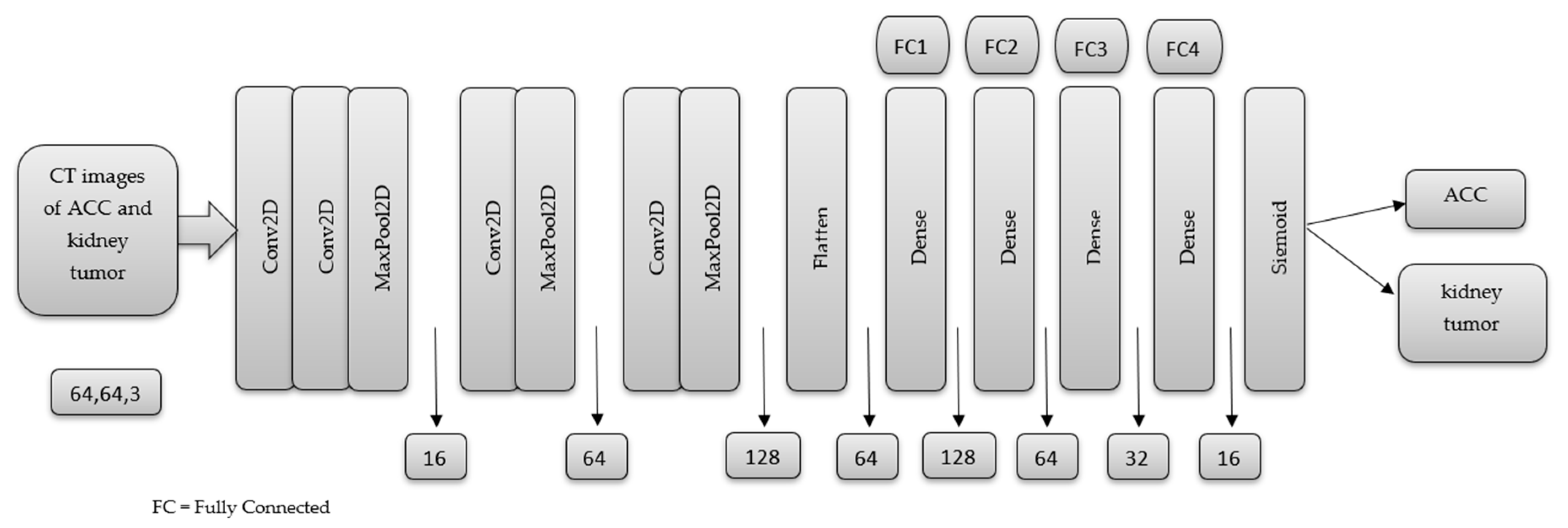
3. Result and Discussion
3.1. Performance Evaluation Metrics
| Precision % |
Sensitivity % |
Specificity % |
F1 Score % |
Accuracy % |
|
|---|---|---|---|---|---|
| ACC | 97.00 | 94.00 | 96.80 | 96.00 | 95.65 |
| Kidney tumor | 95.00 | 97.00 | 94.50 | 96.00 |
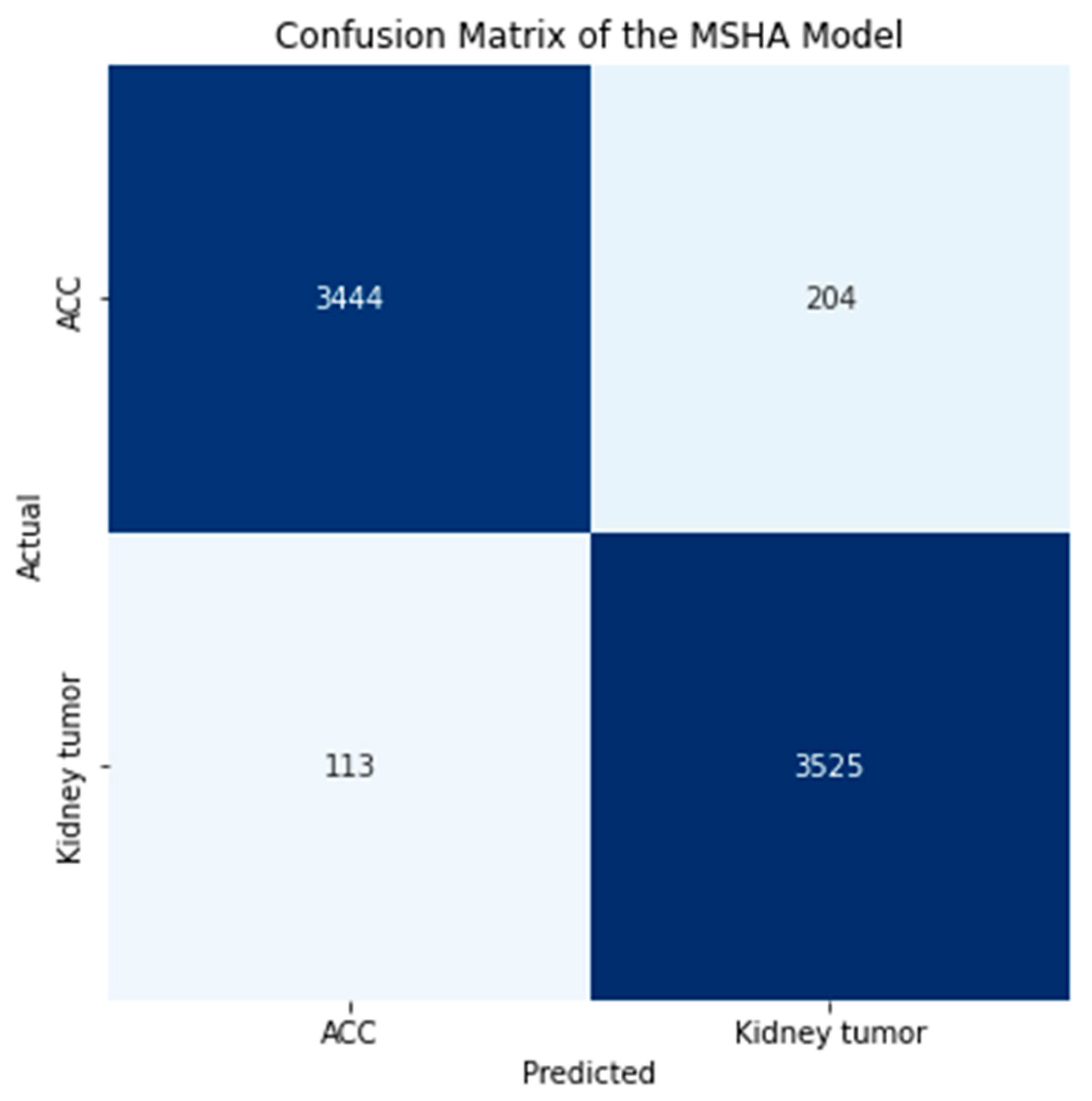
3.2. Confusion Matrix
3.3. Learning Curve
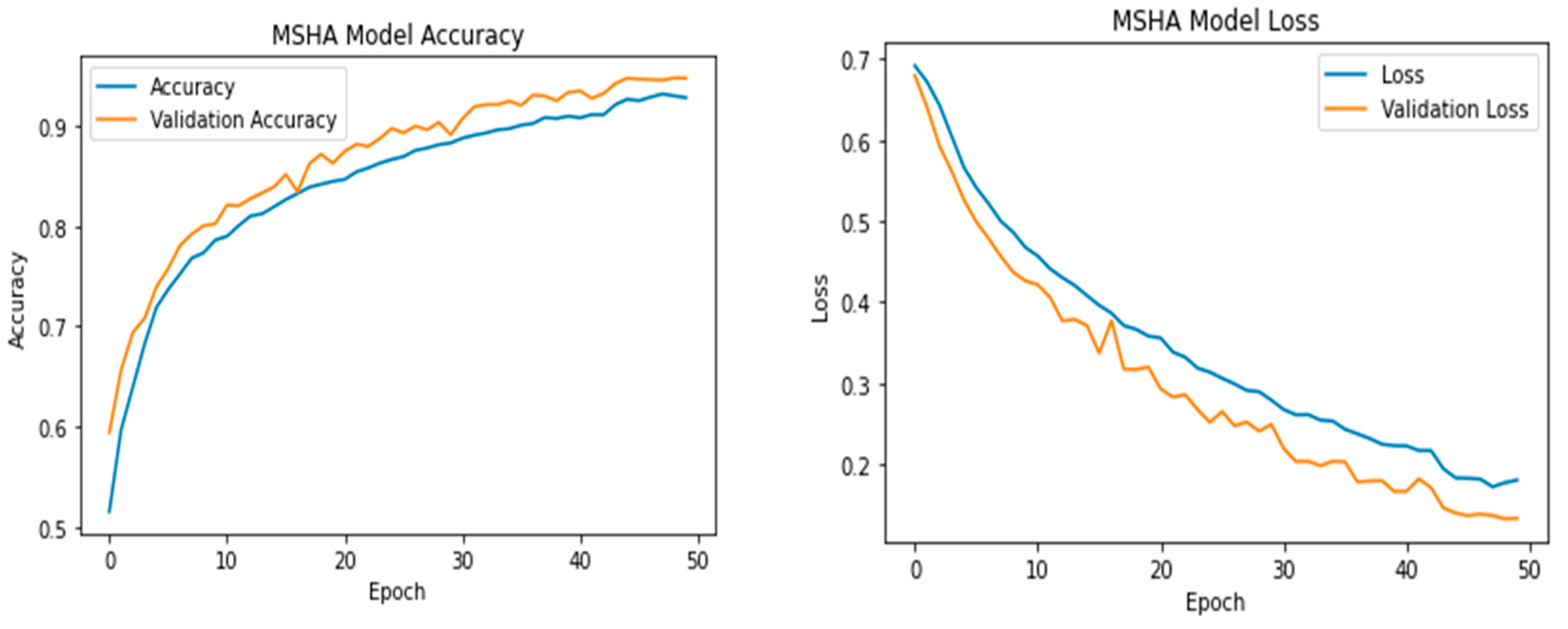
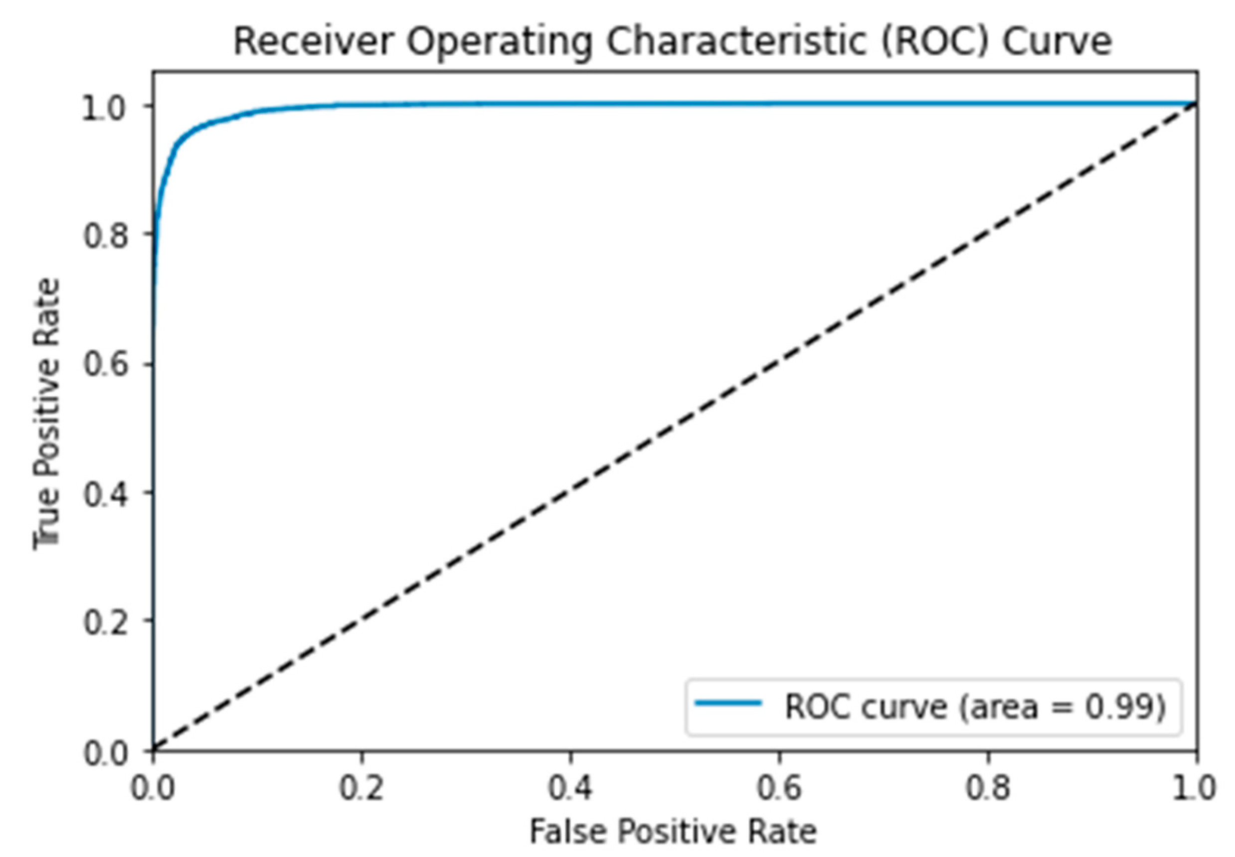
3.4. Receiver Operating Characteristic (ROC) Curve
3.5. Comparative Evaluation with State-of-Art Transfer Learning Techniques
| Models | Precision % |
Sensitivity % |
Specificity % |
F1 Score % |
TP | FP | TN | FN | AUC | Loss | Accuracy % |
|---|---|---|---|---|---|---|---|---|---|---|---|
| MSHA | 96.0 | 96.0 | 96.0 | 96.0 | 3444 | 204 | 3525 | 113 | 0.99 | 0.108 | 96.65 |
| ResNet50 | 66.0 | 66.0 | 66.5 | 66.0 | 2475 | 1173 | 2335 | 1303 | 0.72 | 0.615 | 66.02 |
| VGG16 | 81.0 | 81.0 | 81.0 | 81.0 | 2872 | 776 | 3004 | 634 | 0.90 | 0.424 | 80.65 |
| VGG19 | 81.0 | 80.0 | 80.0 | 80.0 | 2667 | 981 | 3181 | 457 | 0.89 | 0.424 | 80.26 |
| InceptionV3 | 72.0 | 72.0 | 72.0 | 72.0 | 2900 | 748 | 2302 | 1336 | 0.79 | 0.592 | 71.40 |
4. Conclusions
Author Contributions
Funding
Data Availability Statement
Acknowledgments
Conflicts of Interest
References
- Farina, E., Nabhen, J. J., Dacoregio, M. I., Batalini, F., & Moraes, F. Y. (2022). An overview of artificial intelligence in oncology. Future Science OA, 8(4). [CrossRef]
- Talukder, Md. A. (2022). Machine Learning-Based Lung and Colon Cancer Detection Using Deep Feature Extraction and Ensemble Learning. [CrossRef]
- Nandini, B. (2021). Detection of skin cancer using inception V3 and inception V4 Convolutional Neural Network (CNN) for Accuracy Improvement. Revista Gestão Inovação e Tecnologias, 11(4), 1138–1148. [CrossRef]
- Reddy, Y. V., Chandana, G., Redddy, G. C., Kumar, A., Kumar, S., & Ahmed, Dr. S. (2023). Lung cancer detection using Yolo CNN algorithm. International Journal of Research Publication and Reviews, 4(5), 5297–5300. [CrossRef]
- Uzun Ozsahin, D., Onakpojeruo, E. P., Uzun, B., Mustapha, M. T., & Ozsahin, I. (2023). Mathematical assessment of machine learning models used for brain tumor diagnosis. Diagnostics, 13(4), 618. [CrossRef]
- Bi, W. L., Hosny, A., Schabath, M. B., Giger, M. L., Birkbak, N. J., Mehrtash, A., Allison, T., Arnaout, O., Abbosh, C., Dunn, I. F., Mak, R. H., Tamimi, R. M., Tempany, C. M., Swanton, C., Hoffmann, U., Schwartz, L. H., Gillies, R. J., Huang, R. Y., & Aerts, H. J. (2019). Artificial Intelligence in cancer imaging: Clinical challenges and applications. CA: A Cancer Journal for Clinicians. [CrossRef]
- Shi, Y., Qin, Y., Zheng, Z., Wang, P., & Liu, J. (2023). Risk factor analysis and multiple predictive machine learning models for mortality in COVID-19: A Multicenter and multi-ethnic cohort study. The Journal of Emergency Medicine. [CrossRef]
- Nolan, T., & Kirby, J. (2023, June 9). Voxel-level segmentation of pathologically-proven adrenocortical carcinoma with Ki-67 expression (adrenal-ACC-KI67-SEG). Voxel-level segmentation of pathologically-proven Adrenocortical carcinoma with Ki-67 expression (Adrenal-ACC-Ki67-Seg) - The Cancer Imaging Archive (TCIA) Public Access - Cancer Imaging Archive Wiki. https://wiki.cancerimagingarchive.net/pages/viewpage.action?pageId=93257945.
- Singh, Y., Kelm, Z. S., Faghani, S., Erickson, D., Yalon, T., Bancos, I., & Erickson, B. J. (2023). Deep learning approach for differentiating indeterminate adrenal masses using CT imaging. Abdominal Radiology. [CrossRef]
- Avanzo, M., Wei, L., Stancanello, J., Vallières, M., Rao, A., Morin, O., Mattonen, S. A., & El Naqa, I. (2020). Machine and deep learning methods for radiomics. Medical Physics, 47(5). [CrossRef]
- Levy, L., & Tsaltas, J. (2021). Recent advances in benign gynecological laparoscopic surgery. Faculty Reviews, 10. [CrossRef]
- Wei, J., Zhu, R., Zhang, H., Li, P., Okasha, A., & Muttar, A. K. H. (2021). Application of PET/CT image under convolutional neural network model in postoperative pneumonia virus infection monitoring of patients with non-small cell lung cancer. Results in Physics, 26, 104385. [CrossRef]
- Heller, N., Sathianathen, N., Kalapara, A., Walczak, E., Moore, K., Kaluzniak, H., ... & Weight, C. (2019). The kits19 challenge data: 300 kidney tumor cases with clinical context, ct semantic segmentations, and surgical outcomes. arXiv preprint arXiv:1904.00445.
- Subashini, M.; Sahoo, S.; Sunil, V.; Easwaran, S. A Non-Invasive Methodology for the Grade Identification of Astrocytoma Using Image Processing and Artificial Intelligence Techniques. Expert Syst. Appl. 2016, 43, 186–196. [CrossRef]
- Wang, S.; Hamian, M. Skin Cancer Detection Based on Extreme Learning Machine and a Developed Version of Thermal Exchange Optimization. Comput. Intell. Neurosci. 2021, 2021, 9528664. [CrossRef]
- Shorten, C.; Khoshgoftaar, T.M. A survey on image data augmentation for Deep Learning. J. Big Data 2019, 6, 60. [CrossRef]
- Brownlee, J. (2020, August 25). Use early stopping to halt the training of neural networks at the Right Time. MachineLearningMastery.com. https://machinelearningmastery.com/how-to-stop-training-deep-neural-networks-at-the-right-time-using-early-stopping/. (accessed on 28 April 2023).
- 18. Tensorflow callbacks - how to monitor neural network training like a pro. Better Data Science. (n.d.). https://betterdatascience.com/tensorflow-callbacks-how-to-monitor-neural-network-training/#:~:text=If%20a%20value%20of%20the%20evaluation%20metric%20doesn%E2%80%99t,old%20learning%20rate%20multiplied%20by%20a%20user-defined%20factor. (accessed on 28 April 2023).
- Mustapha, M. T.; Ozsahin, D. U.; Ozsahin, I.; Uzun, B. Breast cancer screening based on supervised learning and multi-criteria decision-making. Diagnostics, 2022. 12(6), 1326. [CrossRef]
- Uzun Ozsahin, D.; Mustapha, M. T.; Bartholomew Duwa, B.; Ozsahin, I. Evaluating the performance of deep learning frameworks for malaria parasite detection using microscopic images of peripheral blood smears. Diagnostics, 2022. 12(11), 2702. [CrossRef]
- Seyer Cagatan, A.; Taiwo Mustapha, M.; Bagkur, C.; Sanlidag, T.; Ozsahin, D. U. An alternative diagnostic method for C. Neoformans: Preliminary results of deep-learning based detection model. Diagnostics, 2022. 13(1), 81.
- Muralidhar, K. S. V. Learning curve to identify overfitting and underfitting in machine learning. Medium. Available online: https://towardsdatascience.com/learning-curve-to-identify-overfitting-underfitting-problems-133177f38df5. (accessed on 21 February, 2023).
- Montesinos López, O. A.; Montesinos López, A.; Crossa, J. Overfitting, model tuning, and evaluation of prediction performance. Multivariate Statistical Machine Learning Methods for Genomic Prediction, 2022, 109–139.
- Wolfe, C. R. Using transformers for computer vision. Medium. Available online: https://towardsdatascience.com/using-transformers-for-computer-vision-6f764c5a078b. (accessed on 25 April, 2023).
- Trevisan, V. (2022, March 25). Interpreting ROC curve and ROC AUC for Classification Evaluation. Medium. https://towardsdatascience.com/interpreting-roc-curve-and-roc-auc-for-classification-evaluation-28ec3983f077.
- Brownlee, J. (2020, September 15). ROC curves and precision-recall curves for imbalanced classification. MachineLearningMastery.com. https://machinelearningmastery.com/roc-curves-and-precision-recall-curves-for-imbalanced-classification/.(accessed on 28 April 2023).
- Sabin, J. A. (2022). Tackling implicit bias in health care. New England Journal of Medicine, 387(2), 105–107. https://doi.org/10.1056/nejmp2201180. (accessed on 28 April 2023). [CrossRef]
- Mukherjee, S. (2022, August 18). The annotated resnet-50. Medium. https://towardsdatascience.com/the-annotated-resnet-50-a6c536034758. (accessed on 28 April 2023).
- Understanding VGG16: Concepts, architecture, and performance. Datagen. (2023, May 22). https://datagen.tech/guides/computer-vision/vgg16/.(accessed on 28 April 2023).
- Alake, R. (2020, December 22). Deep learning: Understand the inception module. Medium. https://towardsdatascience.com/deep-learning-understand-the-inception-module-56146866e652. (accessed on 28 April 2023).
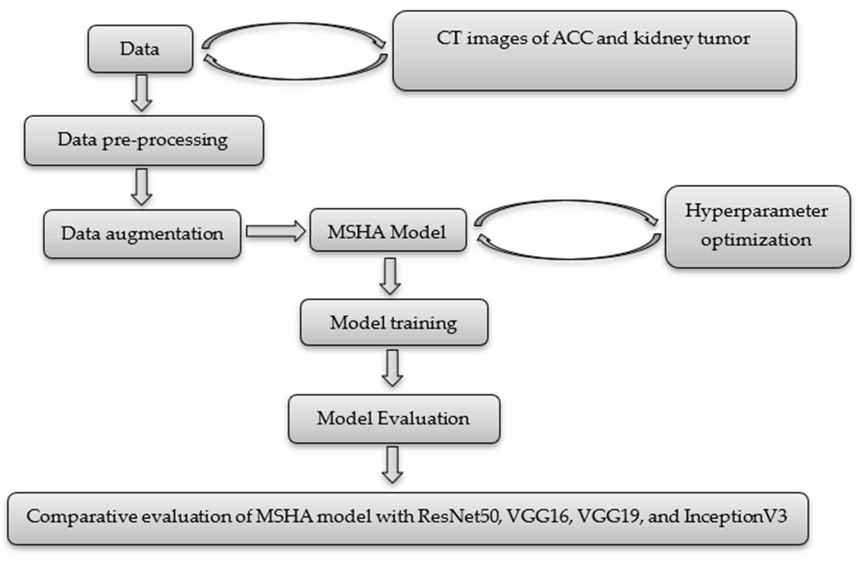
Disclaimer/Publisher’s Note: The statements, opinions and data contained in all publications are solely those of the individual author(s) and contributor(s) and not of MDPI and/or the editor(s). MDPI and/or the editor(s) disclaim responsibility for any injury to people or property resulting from any ideas, methods, instructions or products referred to in the content. |
© 2023 by the authors. Licensee MDPI, Basel, Switzerland. This article is an open access article distributed under the terms and conditions of the Creative Commons Attribution (CC BY) license (http://creativecommons.org/licenses/by/4.0/).


