1. Introduction
Machine learning (ML) is a sub-field of artificial intelligence (AI) that involves the development of algorithms capable of learning patterns and making predictions based on data. It is a broad field that encompasses different approaches and techniques, including deep learning (DL). Deep learning is a subset of ML that involves the use of artificial neural networks (ANN) with multiple layers to learn patterns from data [
1]. The neural networks in deep learning can have many layers, making it possible to extract complex features from data.
One popular application of DL is computer vision, where convolutional neural networks (CNNs) have proven to be very effective in image recognition tasks. CNNs use convolutional layers to extract features from images and pool those features to reduce the dimensionality of the data, allowing them to identify patterns and classify images into different categories [
2].
Pre-trained CNN models are models that have already been trained on large datasets, such as the ImageNet dataset, making them useful for transfer learning on other datasets. Examples of such models are the winners of the ImageNet Large Scale Visual Recognition Challenge (ILSVRC) such as the DenseNets, ResNets, VGGs and others [
3].
However, recently there has been growing interest in a new type of DL architecture called vision transformers (ViTs) [
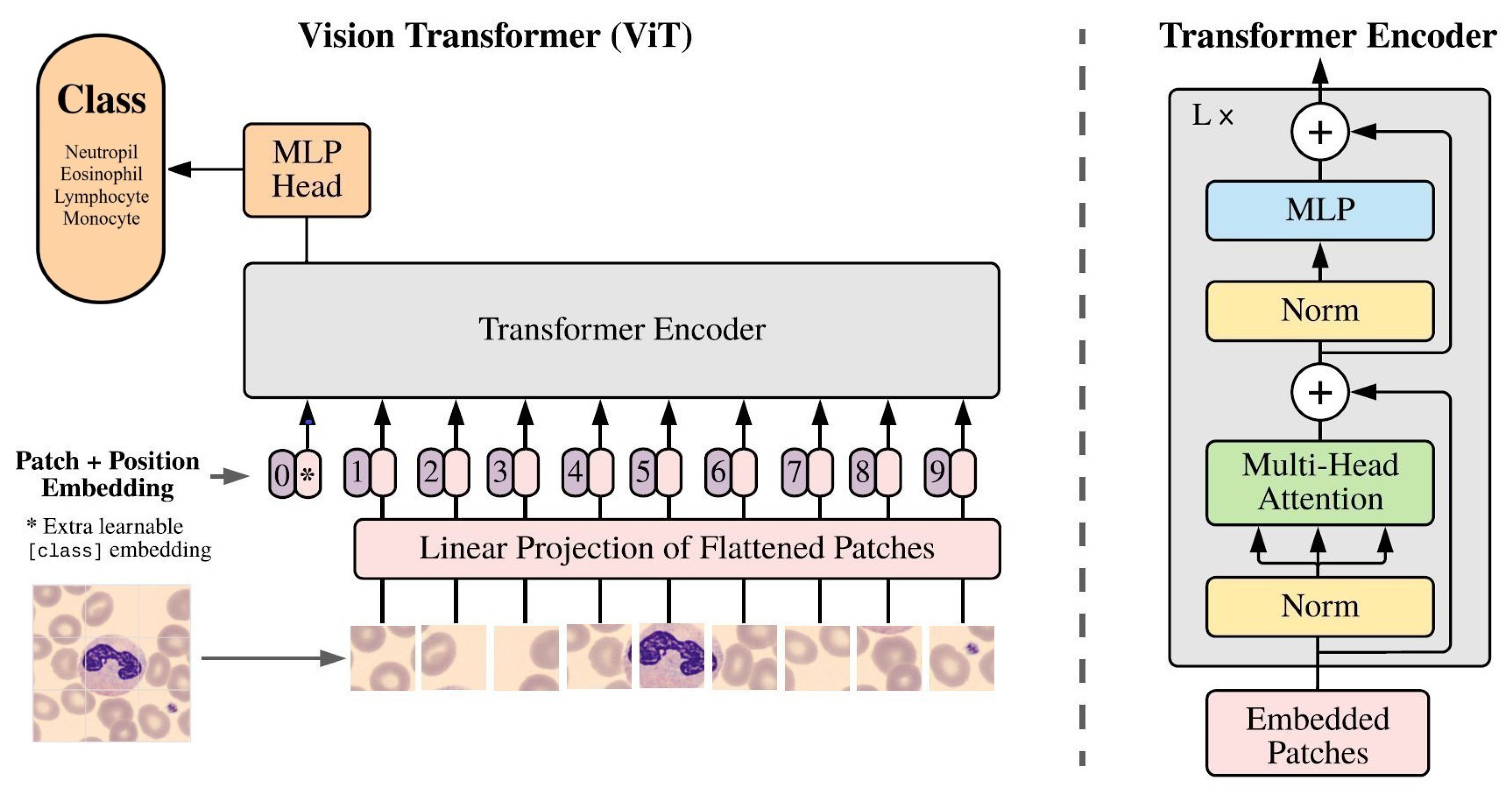
4], which are based on the transformer architecture commonly used in natural language processing (NLP) tasks. The ViT encoder uses a self-attention mechanism to extract features from the input image, allowing the model to look at the entire image at a time and identify important regions of the image. This makes ViTs more efficient in identifying global features in images, such as overall shape and color, and permits it to learn more complex relationships between different parts of the image. Also, ViT use residual links to forward extracted features to an MLP head unaffected with its depth.
This work aims to investigate the performance and optimization learning of both deep neural nets, the ImageNet CNNs and the Google ViT, in classifying four white blood cell (WBC) types "neutrophil, eosinophil lymphocyte and monocyte" by means of transfer learning. This study will use the PBC [
5] and BCCD [
6] datasets, where PBC is a large imbalanced dataset with high-quality images, while BCCD is a small imbalanced dataset with poor-quality images. Data augmentation techniques will be employed to increase the size of the BCCD dataset.
The paper will continue with a literature review of the relevant research related to the detection and classification of WBCs using pre-trained CNNs and ViTs in section 2.
Section 3 will describe the methodology used in this study, while section 4 will present the experimental results obtained using pre-trained ILSVRC models and Google ViT for the blood cell classification. An in-depth analysis of the results will be made in section 5, and the paper will conclude in section 6.
Overall, the paper explores the effectiveness of pre-trained deep learning models in classifying WBC types from peripheral blood smear images. The use of transfer learning and data augmentation techniques is employed to address the imbalanced and poor-quality nature of the datasets. The results of the study can help improve the accuracy and efficiency of WBC classification, which can lead to better diagnosis and treatment of blood disorders.
2. Related Works
There is so many researches and publication works in the autonomous reading of pictures of blood cells in microscopic peripheral blood smears using transfer-based learning from pre-trained ImageNet models and ViTs for small, medium, and large datasets [
7,
8,
9,
10,
11,
12,
13,
14,
15,
16,
17,
18,
19,
20].
However, this work brings novelty in many ways and perspectives when compared to the previous cited works [
7,
8,
9,
10,
11,
12,
13,
14,
15,
16,
17,
18,
19,
20]. First, this work sheds light on as well stresses the significance of data processing techniques, such as data balancing in order to reach better performance and higher accuracy. As well, it demonstrates also the negative impacts of bad data processing habits, such as the overuse of data augmentation methods without the respect of the preservation of an acceptable ratio between original data and its augmented version. Further, it shows clearly how such case could be exaggerated with the event of unclean noisy image data. Finally, it proves the superiority, outperforming, and stability of Google ViT against ImageNet CNNs under such circumstances and conditions.
3. Materials and Methods
This section describes the adopted methodology to classify the four WBC types’ images into different categories. Multi-class classifications have been performed using pre-trained deep neural network models “ImageNet ILSVRC and Google ViT” [
3,
4].
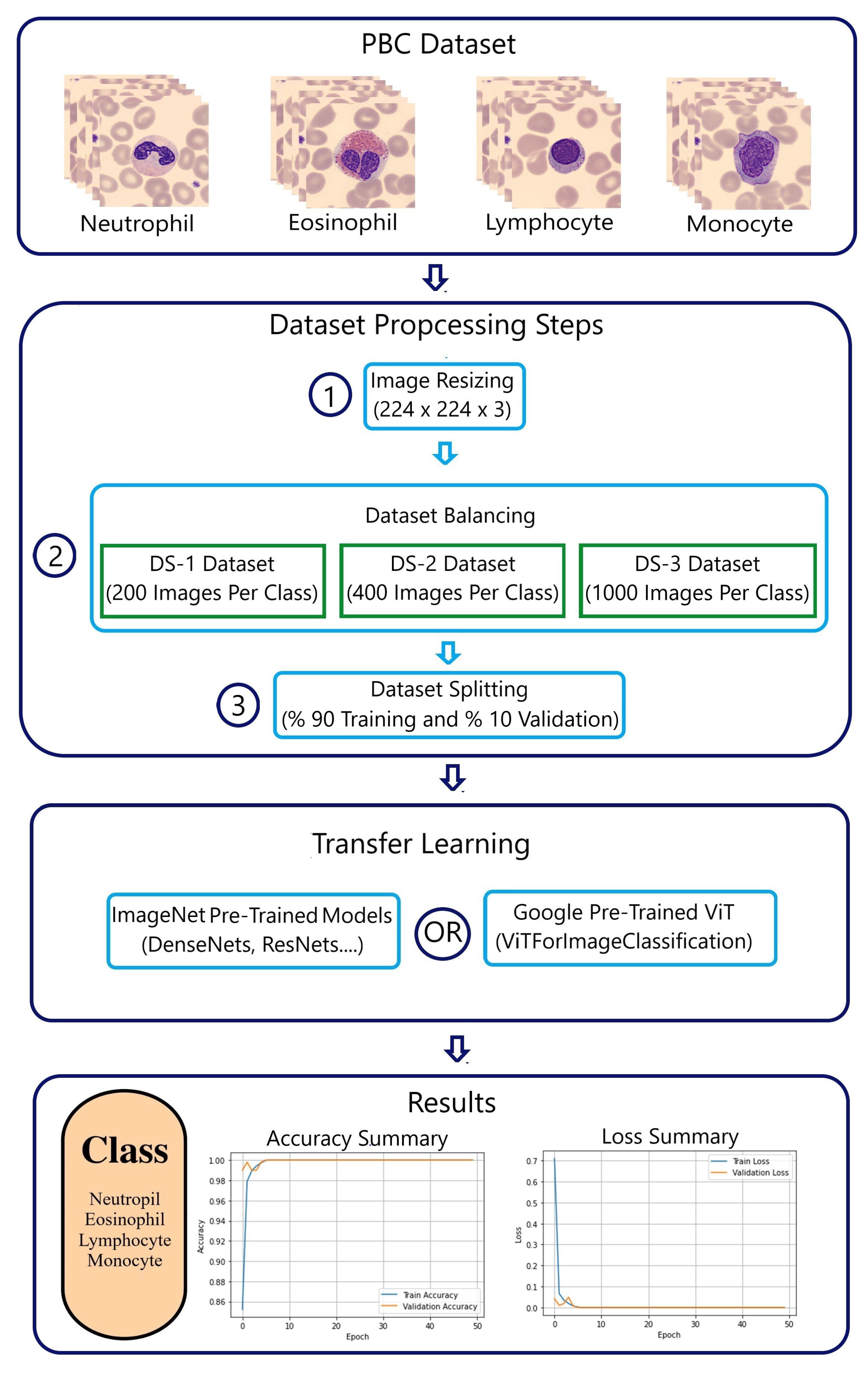
Figure 1 shows a detailed methodology using the PBC dataset [
5].
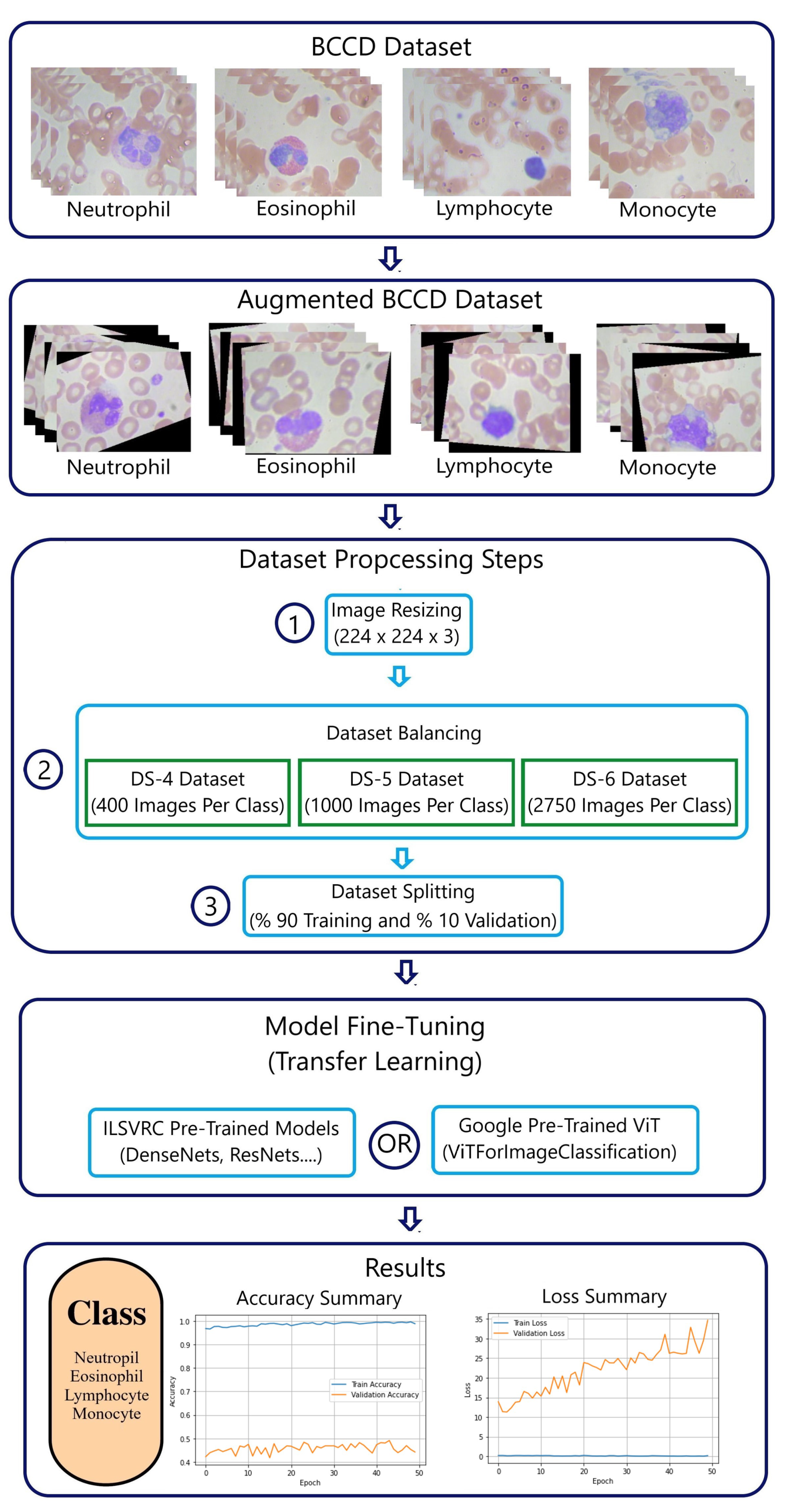
Figure 2 presents a detailed methodology using the BCCD dataset. Additional pre-processing step “data augmentation” is added to increase further the size of the original BCCD dataset [
6].
3.1. PBC and BCCD Datasets
3.1.1. PBC Dataset
The online "peripheral blood cells" dataset, known as the PBC dataset [
5] encloses 17,092 images of eight groups of blood cells: neutrophils, eosinophils, basophils, lymphocytes, monocytes, immature granulocytes, erythroblasts, and platelets (thrombocytes) (
Table 1).
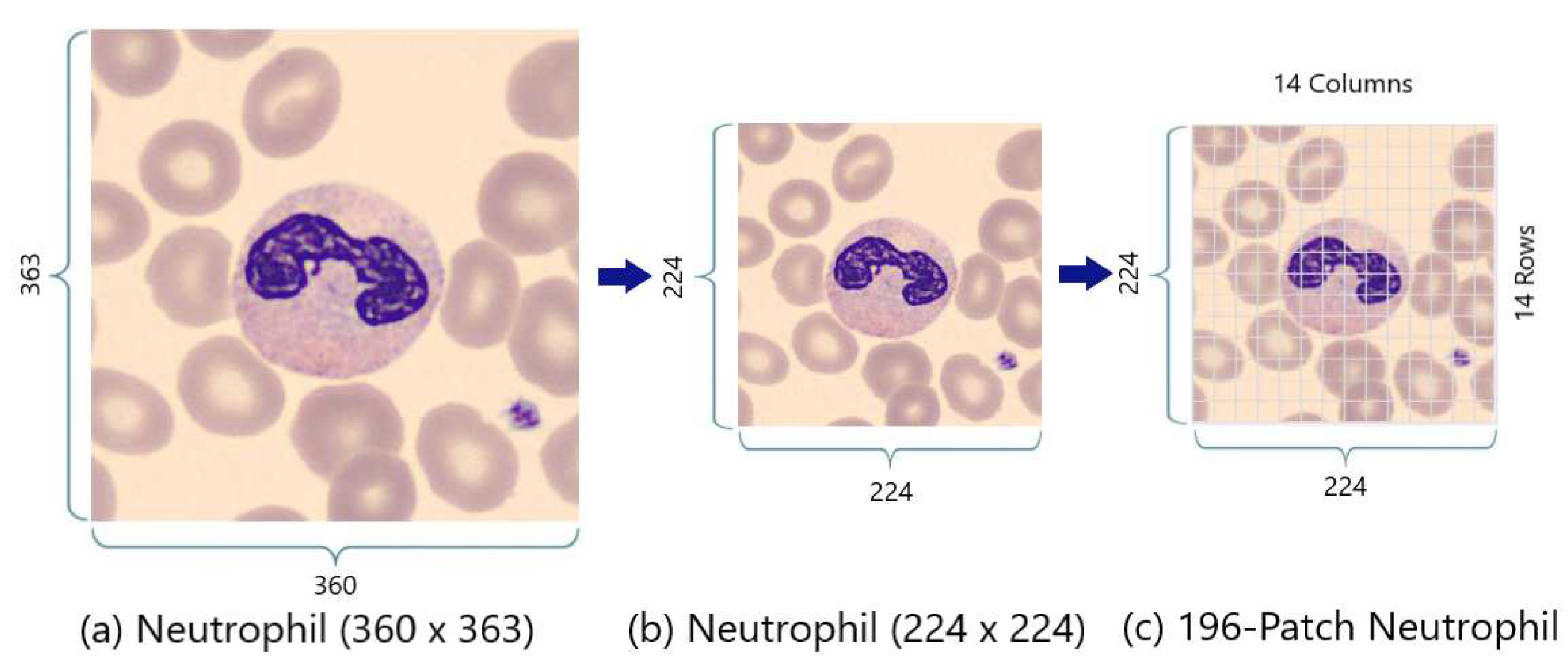
PBC images come with a standard size of 360 ×363 pixels close to the input of the ImageNet models and the Google ViT. This minimizes the impact of images’ downsizing.
3.1.2. BCCD Dataset
The BCCD dataset [
6] originally contains 410 peripheral blood smear images for red blood cells (RBCs), WBCs, and platelets. Images’ format is JPEG with a size of 640x480.
Table 2 [
6] presents a summary of the BCCD distribution of eosinophils, lymphocytes, monocytes and neutrophils.
3.1.3. Datasets Quality and Size
Since the BCCD dataset has only four WBC classes “Neutrophil, Eosinophil, Lymphocyte and Monocyte”, this compels to select only the same four WBC classes from the PBC dataset.
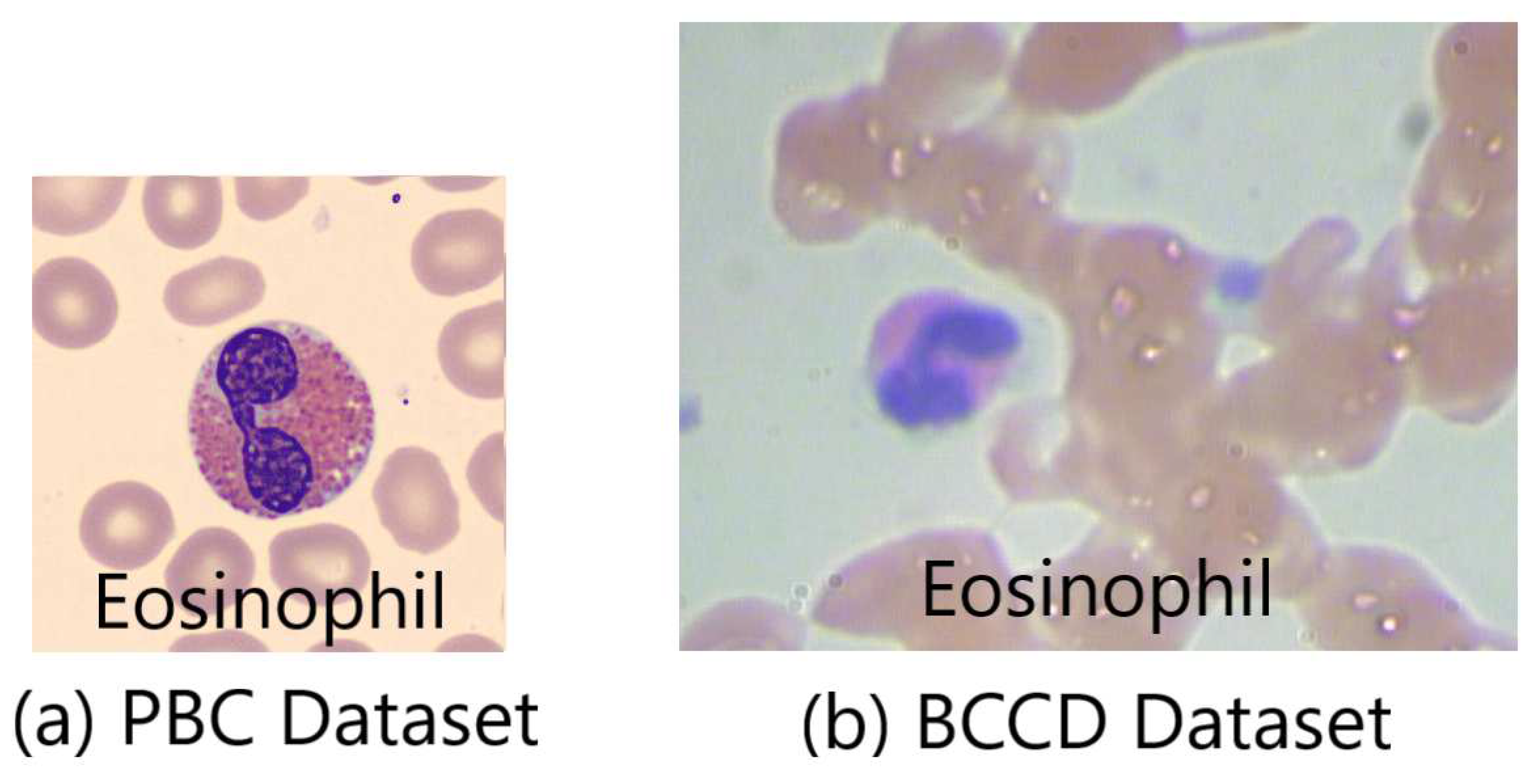
Figure 3 displays the huge difference in images’ quality between the PBC and BCCD datasets. It shows the image of an eosinophil cell. The PBC eosinophil image [
5] demonstrates an image of well-prepared peripheral blood smear, which is free of noise with high resolution and full of details. This return back being automatically prepared and stained by the autostainer Sysmex SP1000i. On the other hand, the BCCD eosinophil image [
6] shows a bad manually prepared, stained and captured peripheral blood smears reflected by noisy images with a poor resolution and few details.
3.2. Datasets Preprocessing
Dataset preprocessing usually consists of many steps including image resizing, data augmentation, data balancing, and data splitting.
3.2.1. PBC Dataset Preprocessing
The PBC dataset preprocessing includes only three steps: image resizing, data balancing, and data splitting. First, images in the PBC dataset needs to be resized to fit the standard “224x224” image input of pre-trained ImageNet ILSVRC and Google ViT models [
3,
4].
Secondly, the analysis of performance demands keeping a minimum number of evaluating metrics during comparison. This target is achieved through balanced datasets with accuracy and loss as assessment tools. Serving this purpose, three balanced datasets (
Table 3), DS-1, DS-2, and DS-3, will represent the PBC dataset.
The final data-preprocessing step involves dividing data into training and validating data with a 10-to-1 fold for each new PBC datasets (
Table 3).
3.2.2. BCCD Dataset Preprocessing
The BCCD dataset preprocessing requires the same PBC dataset preprocessing steps with an additional step “data augmentation” to increase data amount. Table II shows that the number of four WBCs in the BCCD is too small and insufficient. Data augmentation techniques, such as image rotating, and shear, are randomly applied to produce enough data.
Table 4 [
21] represents a summary of the WBCs distribution in the new four created “DS-4, DS-5 and DS-6” BCCD datasets.
3.3. Transfer Learning (TL)
Transfer learning (TL) is a common ML practice in computer vision where a model developed for a task serves as a starting point for a model purposing a second task. Developers build on previous learnings by leveraging already excellent learning models, eliminating the need for a clean slate or starting from scratch. In addition, high performance is realized with small datasets and no expensive supercomputers [
22].
First, in TL, a base network or a model is trained on a base dataset and task. Next, the learned features are transferred to a second target network or model for training on a target dataset and a task. Accordingly, the TL process entails the existence of a pre-trained model, a model formed from an extensive set of reference data to solve a similar problem in another area [
23,
24].
Both pre-trained ImageNet ILSVRC and Google ViT models use MLP head as a classifier. The output layer of the MLP head will be removed and a new output layer will be added representing the four WBC types of the PBC dataset.
3.3.1. ImageNet ILSVRC models
The seven pre-trained ImageNet ILSVRC models shared in this research are DenseNets (DenseNet-169 and DenseNet-201) [
25], InceptionResNet V2 [
26], ResNets (ResNet-50, ResNet-101 and ResNet-152) V2 [
21], and VGG-16 [
27].
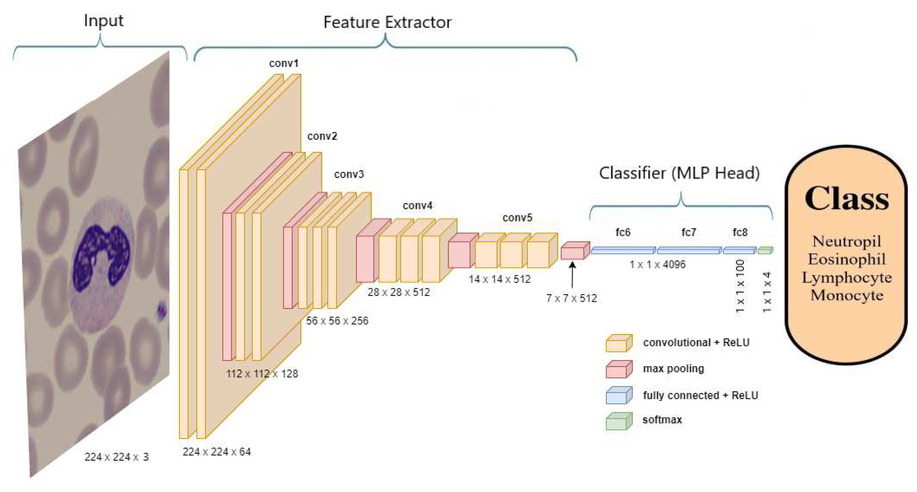
Figure 4 represents a typical example of the transfer learning of the seven pre-trained ImageNet ILSVRC models.
Figure 4 shows the transfer learning process of the VGG-16 model. The weights of all layers of the VGG-16 models will be kept constant “freeze” except the output layer. The parameters of these layers are non-trainable, while the only trainable parameters during the fitting process are only those related to the new 4-class WBC output layer.
3.3.2. Google Vision Transformer (ViT)
Figure 5a,b shows the resizing of the “360 x 363” PBC neutrophil image into “224 x 224” PBC neutrophil image. After that,
Figure 5b,c demonstrates the splitting of the “224 x 224” neutrophil image into 196 patches using the standardized 16x16 patch-size. However,
Figure 3 shows the splitting of neutrophil into 9 patches instead of 196 patches because this aims only for graphical simplification purposes in this figure (
Figure 3).
In the Google ViT transformer similar to the ILSVRC models, only the 1000-class output layer of the MLP head is replaced with the new 4-class WBC output layer.
Figure 6 represents the transfer learning of the Google ViT transformer “ViTForImageClassification”.
However, all the parameters of the vision transformer enter into the training and validating process, and this justifies the longer training time compared to the ILSVRC models.
3.3.3. Trials Setup
The AI tool used in this work is Google Colaboratory, “Google Colab” for short. Google Colab is a product very useful for ML and data analysis allowing data scientists to write and execute python code through an online-hosted Jupyter notebook [
28].
The parameters kept constant during the trials are the “Adam” data optimizer, the “Categorical Cross-Entropy” loss function, the “Accuracy” metric, the “10” epochs’ number, and the “10-to-1 Fold” training-to-validating ratio.
3.3.4. Evaluation Metrics
The comparison of the ImageNet models and Google ViT will be based on two types of learning curves: optimization and performance.
Optimization curves are types of learning curves calculated on the metric by which the model’s parameters are being optimized, such as loss or Mean Squared Error (MSE).
In this work, “Categorical Cross-Entropy” [
29] is used as a loss function. Cross-entropy loss is used when adjusting model weights during training aiming to minimize the loss. This means the smaller the loss the better the model. A perfect model has a cross-entropy loss of zero. Cross-entropy [
29] is defined in the equation
1 as:
Where is the truth label and is the Softmax probability for the ith class. Moreover, there are also two essential correlated terms associated with optimization curves: variance and overfitting.
Variance [
30,
31,
32] is the difference in fits between data sets “training and validating”. A high variance typically occurs when the model is too complex and does not reflect the simpler real patterns existing in the data. Variance is calculated by using the equation
2:
Where equals each value in the dataset, is the mean of all values in the dataset, and N is the number of values in the dataset.
The training loss (TL) indicates how well the model is fitting the training data, while the validation loss (VL) indicates how well the model fits new data. Variance is correlated to the loss difference (LD), which is the difference between VL and TL. LD is calculated using the equation
3:
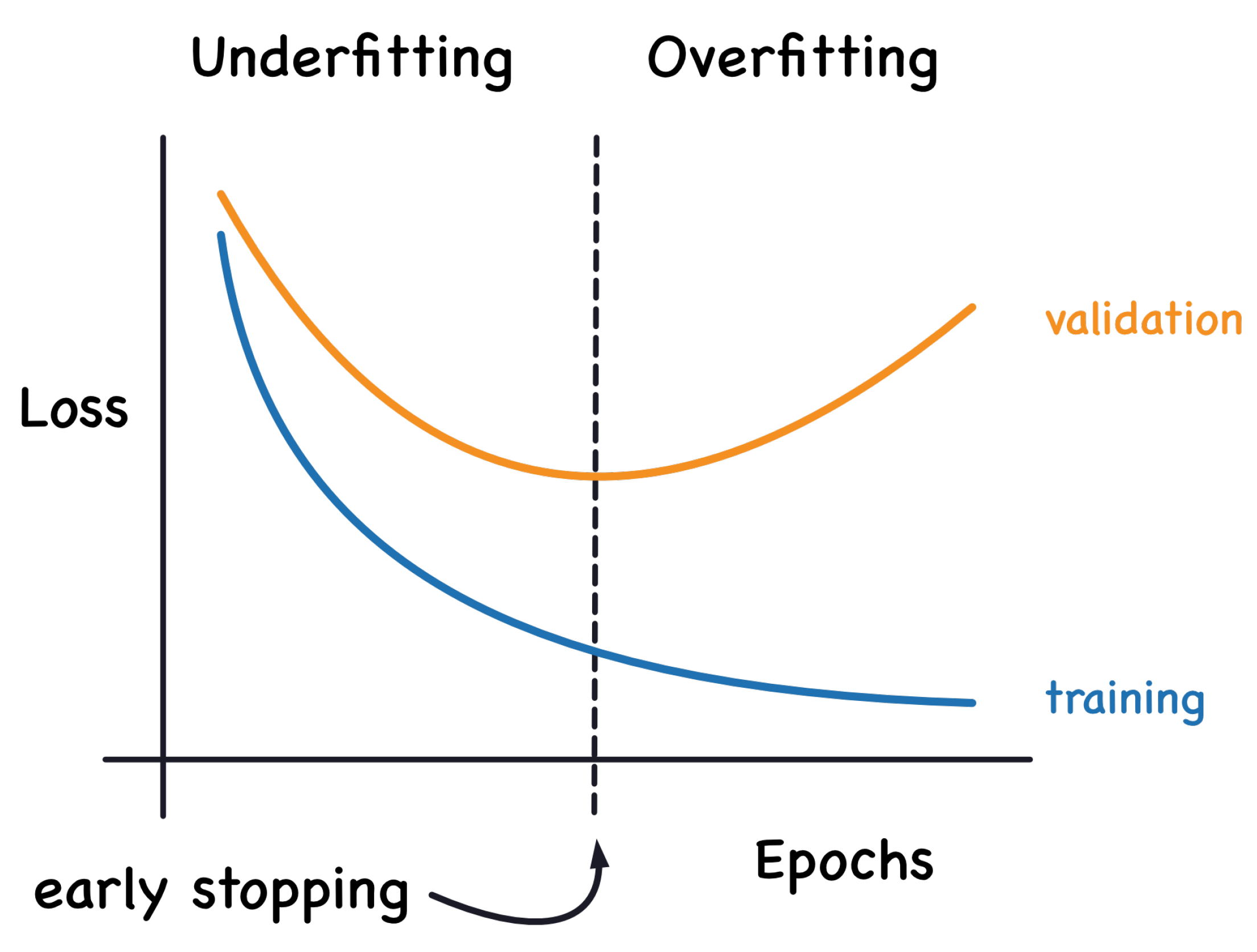
Figure 7 [
33] explains the underfitting and overfitting problems in relation training and validation losses. When the deep learning algorithm captures well the training data but performs poorly on new data, it is unable to generalize, and this is known as overfitting. The greater the variance of a model, the greater it overfits the training data
As for performance learning, accuracy represents the ratio of true predicted classes to the total number of samples evaluated [
34]. Equation
4 [
34] demonstrates this computational process:
Where TN and TP account for successfully classified negative and positive cases, correspondingly. As well, FN and FP report the number of misclassified positive and negative cases respectively.
Another parameter that will be used for performance assessment is the accuracy difference (AD)
5, the difference between training accuracy (TA) and validating accuracy (VA).
4. Results
This section explains the experimental results of classifying WBC cells using seven pre-trained ImageNet ILSVRC models and the Google ViT "ViTForImageClassification" transformer. The experiments were conducted on both the online peripheral blood smear PBC and BCCD datasets. The PBC dataset is characterized being a large imbalanced dataset with standardized consistent high-quality images full of details. Whereas, the BCCD dataset is a small imbalanced dataset with blurring and noisy images due to the fact being manually prepared, stained, and captured.
In these experiments, the PBC imbalanced dataset is represented by three balanced datasets: DS-1 (200 images per class), DS-2 (400 images per class), and DS-3 (1,000 images per class) datasets. Due to the small size of the BCCD dataset, data augmentation techniques are applied to increase the amount of data. Thus, the imbalanced BCCD dataset is embodied by three balanced datasets: DS-4 (400 images per class), DS-5 (1,000 images per class), and DS-6 (2,750 images per class) datasets. The datasets balancing is purposing to evaluate ImageNet CNNs and Google ViT based on minimal metrics "accuracy and loss".
4.1. PBC Datasets Results
Table 5 shows the tenth epoch validating accuracy and loss (VA and VL) values of seven pre-trained ImageNet ILSVRC models versus Google ViT. Google ViT exhibits exceptional stable performance over all ImageNet ILSVRC models. The Google ViT transformer has a validation accuracy of 100 percent and a validation loss close to zero when fitted with three PBC datasets (DS-1, DS-2, and DS-3).
As shown in
Table 6, Google ViT again outperforms all ILSVRC models with a zero accuracy difference (AD) value, which equals the difference between training and validating accuracies (TA and VA).
Table 7 shows clearly the overfitting problem development in all ILSVRC models due to high variances caused by high LD values when fitted by the DS-1 and DS-1 datasets. However, the size of the small and medium datasets "DS-1 and DS-2" has no impact on the behavior of Google ViT, which shows great results in such cases.
Finally, the large number of Google ViT trainable parameters compared to all ILSVRC models during the transfer learning process explains its need for additional computational resources and a longer training and validating time.
4.2. BCCD Datasets Results
Table 8 shows the tenth epoch validating accuracy and loss (VA and VL) values of seven pre-trained ImageNet ILSVRC models versus Google V. The models are fitted with the three BCCD datasets (DS-4, DS-5, and DS-6). Google ViT demonstrates a better performance over all ImageNet ILSVRC models.
The Google ViT transformer has reached an 88.6 % validation accuracy and a validation loss close to one when fitted with the BCCD DS-6 dataset. By comparison, fitting with the DS-6 dataset, all ImageNet ILSVRC display a catastrophic optimization learning and performance. This returns back to the great amount of noise caused by the overuse of data augmentation and poor quality of images of original BCCD dataset.
Table 8 shows the tenth epoch validating accuracy and loss (VA and VL) values of seven pre-trained ImageNet ILSVRC models versus Google V. The models are fitted with the three BCCD datasets (DS-4, DS-5, and DS-6). Google ViT demonstrates a better performance over all ImageNet ILSVRC models.
As shown in
Table 9, Google ViT, fitted with the DS-6, again outperforms with a +11.64 % accuracy difference (AD) value, which is far away from any AD achieved by all ILSVRC models.
Table 10 demonstrates clearly that Google ViT, fitted with the DS-6, again outperforms with around 1 % loss difference (LD) value, which is lower than any LD attained by all ILSVRC models
Thus, the
Table 9 and
Table 10 come to stress the same facts and conclusion drawn conclusion from the Table VIII.
5. Discussion
In general, the experimental trials conducted in this study prove the superiority of Google ViTs over ImageNet CNNs in the classification task of peripheral blood smear WBC types since it has a higher immunity against noise and requires a lesser amount of data.
The excellent consistent high-quality images of the PBC dataset have allowed Google ViT to prove its superiority and stability over ImageNet CNNs especially in the case of a lesser amount of image data, such as the DS-1 dataset. This consequently addresses a major challenge in the AI world and faced by most data scientists “data scarcity” when applying deep learning nets. Secondly, the exaggeration of noise level through the application of data augmentation on poor quality images of the BCCD dataset has permitted Google ViT to prove its benefit, applicability, and higher immunity against such challenge.
This all could be justified and returns back primarily to the capability of Google ViT to extract both global and local features, and use residual connections to transfer them to the MLP head without being impacted by its depth. Whereas, the ImageNet CNNs extract in principle local features and in a much less manner global ones, and is highly influenced with the depth increase.
However, the transfer learning of Google ViT needs more time and computational power resources by comparison to the ImageNet CNNs.
6. Conclusions
The work compared comprehensively the performance of Google ViT facing 11 traditional DL ImageNet CNNs in classifying four types of WBCs from two online peripheral blood smear datasets, the PBC and BCCD datasets. The PBC dataset contains 17,092 high-quality images of eight groups of blood cells and is presented in this work through three balanced datasets (DS-1, DS-2, and DS-3). The use of the three balanced-PBC datasets consequently proves the benefit and optimal performance of Google ViT against ImageNet CNNs in the case of data shortage. On the other hand, the BCCD dataset encompasses 349 poor-quality images of four types of WBCs and is presented with three balanced datasets (DS-4, DS-5, and DS-6) created through the application of data augmentation techniques. This application led to the introducing of a large amount of noise within the data. Another time, such application demonstrated the capability, stability and immunity of Google ViT facing noisy data by comparison to ImageNet CNNs. In a nutshell, ViT proves its optimal performance in the case of data insufficiency and the presence of unclean data.
In the future, the adopted methodology in this paper will be furtherly examined and investigated in other medical imaging applications, such as radiology, endoscopy, ophthalmology and others.
Author Contributions
For research articles with several authors, a short paragraph specifying their individual contributions must be provided. The following statements should be used “Conceptualization, M.A. and F.D.; methodology, M.A. and F.D.; software, M.A.; validation, M.A.; formal analysis, M.A., F.D. and I.A.; investigation, M.A.; resources, M.A. and F.D.; data curation, M.A.; writing—original draft preparation, M.A. and F.D.; writing—review and editing, M.A., F.D. and I.A.; supervision, F.D. and I.A.; project administration, F.D. and I.A.; funding acquisition, F.D. and I.A. All authors have read and agreed to the published version of the manuscript.
Data Availability Statement
The data used in this paper are publicly available.
Acknowledgments
This work is partially supported by grant PID2021-126701OB-I00 funded by MCIN/AEI/10.13039/501100011033 and by “ERDF A way of making Europe”.
Conflicts of Interest
The authors declare that the research was conducted in the absence of any commercial or financial relationships that could be construed as a potential conflict of interest.
References
- C. Mishra and D. L. Gupta, “Deep machine learning and neural networks: An overview,” IAES Int. J. Artif. Intell. (IJ-AI), vol. 6, no. 2, p. 66, 2017. [CrossRef]
- T. A. Sadoon and M. H. R. Ali, “An Overview of Medical Images Classification based on CNN,” Int. J. Curr. Eng. Technol., vol. 10, no. 06, pp. 900–905, 2020. [CrossRef]
- O. Russakovsky et al., “ImageNet large scale visual recognition challenge,” Int. J. Comput. Vis., vol. 115, no. 3, pp. 211–252, 2015. [CrossRef]
- A. Dosovitskiy et al., “An image is worth 16x16 words: Transformers for image recognition at scale,” arXiv, 2020. [CrossRef]
- A. Acevedo, A. Merino, S. Alférez, Á. Molina, L. Boldú, and J. Rodellar, “A dataset of microscopic peripheral blood cell images for development of automatic recognition systems,” Data Brief, vol. 30, no. 105474, p. 105474,2020. [CrossRef]
- S. Cheng, BCCD Dataset: BCCD (Blood Cell Count and Detection) Dataset is a small-scale dataset for blood cells detection. https://github.com/Shenggan/BCCD_Dataset.
- M. Sharma, A. Bhave, and R. R. Janghel, “White blood cell classification using convolutional neural network,” in Advances in Intelligent Systems and Computing, Singapore: Springer Singapore, 2019, pp. 135–143. [CrossRef]
- M. M. Alam and M. T. Islam, “Machine learning approach of automatic identification and counting of blood cells,” Healthc. Technol. Lett., vol. 6, no. 4, pp. 103–108, 2019.
- A. Acevedo, S. Alférez, A. Merino, L. Puigví, and J. Rodellar, “Recognition of peripheral blood cell images using convolutional neural networks,” Comput. Methods Programs Biomed., vol. 180, no. 105020, p. 105020, 2019.
- C. Jung, M. Abuhamad, J. Alikhanov, A. Mohaisen, K. Han, and D. Nyang, “W-Net: A CNN-based architecture for white blood cells image classification,” arXiv, 2019. [CrossRef]
- Y. Wang, C. Wang, L. Luo and Z. Zhou, "Image Classification Based on transfer Learning of Convolutional neural network," 2019 Chinese Control Conference (CCC), Guangzhou, China, 2019, pp. 7506-7510. [CrossRef]
- S. Abou El-Seoud, M. H. Siala, and G. McKee, “Detection and classification of white blood cells through deep learning techniques,” Int. J. Onl. Eng., vol. 16, no. 15, p. 94, 2020. [CrossRef]
- A. T. Sahlol, P. Kollmannsberger, and A. A. Ewees, “Efficient classification of white Blood Cell Leukemia with improved swarm optimization of deep features,” Sci. Rep., vol. 10, no. 1, p. 2536, 2020. [CrossRef]
- K. Almezhghwi and S. Serte, “Improved classification of white blood cells with the generative adversarial network and deep convolutional neural network,” Comput. Intell. Neurosci., vol. 2020, p. 6490479, 2020. [CrossRef]
- S. Tavakoli, A. Ghaffari, Z. M. Kouzehkanan, and R. Hosseini, “New segmentation and feature extraction algorithm for classification of white blood cells in peripheral smear images,” Sci. Rep., vol. 11, no. 1, p. 19428, 2021. [CrossRef]
- K. T. Navya, K. Prasad and B. M. K. Singh, "Classification of blood cells into white blood cells and red blood cells from blood smear images using machine learning techniques," 2021 2nd Global Conference for Advancement in Technology (GCAT), Bangalore, India, 2021, pp. 1-4. [CrossRef]
- Z. Jiang, Z. Dong, L. Wang, and W. Jiang, “Method for diagnosis of acute lymphoblastic leukemia based on ViT-CNN ensemble model,” Comput. Intell. Neurosci., vol. 2021, p. 7529893, 2021. [CrossRef]
- P. Cho, S. Dash, A. Tsaris, and H.-J. Yoon, “Image transformers for classifying acute lymphoblastic leukemia,” in Medical Imaging 2022: Computer-Aided Diagnosis, 2022. [CrossRef]
- N. Sengar, R. Burget, and M. K. Dutta, “A vision transformer based approach for analysis of plasmodium vivax life cycle for malaria prediction using thin blood smear microscopic images,” Comput. Methods Programs Biomed., vol. 224, no. 106996, p. 106996, 2022. [CrossRef]
- Sun, T., Zhu Q., Yang J., and Zeng L., “An improved Vision Transformer model for the recognition of blood cells,” Sheng Wu Yi Xue Gong Cheng Xue Za Zhi, vol. 39, no. 6, pp. 1097–1107, 2022. [CrossRef]
- K. He, X. Zhang, S. Ren, and J. Sun, “Deep residual learning for image recognition,” in 2016 IEEE Conference on Computer Vision and Pattern Recognition (CVPR), 2016. [CrossRef]
- J. Puigcerver et al., “Scalable transfer learning with expert models,” Computing Research Repository (CoRR), 2020. [CrossRef]
- H. E. Kim, A. Cosa-Linan, N. Santhanam, M. Jannesari, M. E. Maros, and T. Ganslandt, “Transfer learning for medical image classification: a literature review,” BMC Med. Imaging, vol. 22, no. 1, p. 69, 2022. [CrossRef]
- K. Weiss, T. M. Khoshgoftaar, and D. Wang, “A survey of transfer learning,” J. Big Data, vol. 3, no. 1, 2016. [CrossRef]
- G. Huang, Z. Liu, L. Van Der Maaten and K. Q. Weinberger, "Densely Connected Convolutional Networks," 2017 IEEE Conference on Computer Vision and Pattern Recognition (CVPR), Honolulu, HI, USA, 2017, pp. 2261-2269. [CrossRef]
- C. Szegedy, V. Vanhoucke, S. Ioffe, J. Shlens and Z. Wojna, "Rethinking the Inception Architecture for Computer Vision," 2016 IEEE Conference on Computer Vision and Pattern Recognition (CVPR), Las Vegas, NV, USA, 2016, pp. 2818-2826. [CrossRef]
- K. Simonyan and A. Zisserman, “Very deep convolutional networks for large-scale image recognition,” Computing Research Repository (CoRR), 2014. [CrossRef]
- E. Bisong, “Google Colaboratory,” in Building Machine Learning and Deep Learning Models on Google Cloud Platform, Berkeley, CA: Apress, 2019, pp. 59–64. [CrossRef]
- P. Li et al., “Improved categorical cross-entropy loss for training deep neural networks with noisy labels,” in Pattern Recognition and Computer Vision, Cham: Springer International Publishing, 2021, pp. 78–89. [CrossRef]
- P. Mehta et al., “A high-bias, low-variance introduction to Machine Learning for physicists,” Phys. Rep., vol. 810, pp. 1–124, 2019. [CrossRef]
- S. Doroudi, “The bias-variance tradeoff: How data science can inform educational debates,” AERA Open, vol. 6, no. 4, p. 233285842097720, 2020. [CrossRef]
- Y. Dar, V. Muthukumar, and R. G. Baraniuk, “A farewell to the bias-variance tradeoff? An overview of the theory of overparameterized machine learning,” arXiv [stat.ML], 2021. [CrossRef]
- R. Holbrook, “Overfitting and Underfitting: Improve performance with extra capacity or early stopping,” Kaggle. [Online]. Available: https://www.kaggle.com/code/ryanholbrook/overfitting-and-underfitting. [Accessed: 01-October-2023].
- L. Alzubaidi et al., “Review of deep learning: concepts, CNN architectures, challenges, applications, future directions,” J. Big Data, vol. 8, no. 1, p. 53, 2021. [CrossRef]
|
Disclaimer/Publisher’s Note: The statements, opinions and data contained in all publications are solely those of the individual author(s) and contributor(s) and not of MDPI and/or the editor(s). MDPI and/or the editor(s) disclaim responsibility for any injury to people or property resulting from any ideas, methods, instructions or products referred to in the content. |
© 2023 by the authors. Licensee MDPI, Basel, Switzerland. This article is an open access article distributed under the terms and conditions of the Creative Commons Attribution (CC BY) license (http://creativecommons.org/licenses/by/4.0/).
