Improving Semantic Segmentation Performance in Underwater Images

Preprint

Article

Improving Semantic Segmentation Performance in Underwater Images

Altmetrics

Downloads

Views

Comments

A peer-reviewed article of this preprint also exists.

Alexandra Pereira Nunes^*

,Aníbal Matos

Alexandra Pereira Nunes^*

,Aníbal Matos

This version is not peer-reviewed

Submitted:

26 October 2023

Posted:

27 October 2023

You are already at the latest version

Alerts

Abstract

Nowadays, semantic segmentation is increasingly used in exploration by underwater robots, for example in autonomous navigation, so that the robot can recognise the nature and elements of its environment during the mission and act according to this classification to avoid collisions. Other applications can be found in the search for archaeological artefacts, in the inspection of underwater structures or in species monitoring. Therefore, it is necessary to try to improve the performance in these tasks as much as possible. To this end, we compare some methods for improving image quality and for data augmentation and test whether higher performance metrics can be achieved with both strategies. The experiments are performed with the SegNet implementations and the SUIM dataset with 8 common underwater classes to compare the obtained results with the already known ones. The results obtained with both strategies show that they are beneficial and lead to better performance results by achieving a mean IoU of 56% and an increased overall accuracy of 81.8%. The single result shows that there are 5 classes with an IoU value above 60% and only one class with an IoU value below 30%, which is a more reliable result and easier to use in real contexts.

Keywords:

Subject: Engineering - Marine Engineering

1. Introduction

Semantic segmentation is an important task for the various fields of robotics, which often relies on visual data from cameras. Nowadays, it is increasingly used in robotic exploration of the underwater world, for example in autonomous navigation, so that the robot can recognise the nature and elements of its environment during the mission and act according to this classification to avoid collisions, for example, as well as in object recognition and finding archaeological artefacts or even inspecting underwater structures such as platforms, cables or pipelines. Other applications can be found in marine biology and ecology in identifying species and monitoring their growth, but also in the search and rescue of missing persons or the recovery of parts of ships, or in military defence through the detection and classification of mines. The main objective of this task is to label each pixel of an image with a corresponding class of the represented image, which is a dense classification, and often it is difficult to obtain good results in terms of prediction. In conventional approaches, there are some problems with the accuracy of the results because the data obtained in underwater environments have challenges such as colour distortion, low contrast, noise or uneven illumination, and for these reasons some important information is lost. In addition, traditional methods generally do not have high transferability or robustness, so the segmentation effect of a single traditional method is in the majority of the cases poor [1]. Therefore, it is necessary to resort to advanced approaches, often incorporating Deep Learning [2], in order to to better overcome these challenges of the underwater environment [3,4,5]. However, for these methods to perform well on this type of task that requires training models, appropriate datasets must be used. However, one of the main problems with visual methods in this area is often the lack of complete datasets or with multiple images to consider for different contexts or classes [6,7,8,9]. When there are existing suitable datasets for the general underwater context, they often do not have masks with the ground truth label [10], which is a challenge when it is necessary to manually label them. In a previous study by the authors, the SUIM dataset [11] was selected to comparatively test different machine learning approaches (SegNet [12], Pyramid Scene Parsing Network - PSPNET [13] and two versions of Fully Convolutional Networks - FCNN [14]) for semantic segmentation. This dataset was chosen because it contains 7 common classes of the underwater world with different perspectives and visual conditions. In this research [15], the Segnet implementation, which is a deep, fully convolutional neural network architecture for pixel-level semantic segmentation and designed to be efficient in terms of both memory and computation time, stands out in terms of key performance metrics. Thus, the overall accuracy, mean accuracy and mean Intersection over Union (IoU) achieve 80%, 64% and 52% respectively, but show lower performance when we analyse the results of the individual classes, with only three of the overall classes achieving more than 60% and two classes achieving less than 30%, with one train large for 100 evaluations. Although the results obtained are not bad in real contexts, they could be dangerous to work with in a real mission and the question arises: "Can we achieve higher accuracy in semantic segmentation?". According to the literature, it is possible to improve the results of semantic segmentation by adjusting the parameters of the model, resorting to some image enhancement techniques, increasing the number of images for training, using more balanced datasets, etc [16,17]. The first goal was to find the right parameters and this was achieved in the first iteration. Now the next strategies need to be tested to see if they are successful in the underwater environment.

Therefore, the main purpose of this work is to verify if there are some approaches commonly used in outdoor environments that allow to improve the results in terms of accuracy and how much this improvement is, comparing some methods to improve the image quality and some data augmentation strategies. The idea is that in the final of this work to know how to build a dataset more balanced and without less effort in collecting data as it is already challenging and expensive in terms of time and cost.

This paper is arranged as follows: Section 2 describes the background of this work with the explanation of the previously obtained results, i.e. the starting point of this study. Section 3 describes the main methods used to improve the quality of the underwater images and some approaches to expand the number of samples in a dataset. Next, the Section 4 presents the main findings in terms of accuracy and visual results and some discussion about them, and finally, in the Section 5 presents the main conclusions and some ideas for future work.

2. Background

Semantic segmentation involves labelling all objects of the same class, and when used with machine learning, the system is trained with already segmented datasets to accurately identify elements and segment an unknown set of images. As mentioned earlier, the authors conducted a detailed comparative study of different implementations for semantic segmentation applications in an underwater context in a first paper [15]. For this, after reviewing the available online data, we used the SUIM dataset, which is one of the most complete and could be useful in these scenarios, although it does not yet contain all the intended objects. It is not a large dataset as it is not easy to obtain underwater images for these scenarios, but it provides different perspectives as well as colour and size information. Another important aspect of this dataset is that it contains the ground truth for the different images, i.e. masks with the pixels labelled with the classes. There are 8 classes: Waterbody (Class 0), Human Divers (Class 1), Robots or Instruments (Class 2), Reefs and Invertebrates (Class 3), Plants (Class 4), Wrecks or Ruins (Class 5), Fish and Vertebrates (Class 6), and Seabed and Rocks (Class 7), but with a different number of samples for each class, which leads to an unbalanced dataset and could be a problem in the training phase. 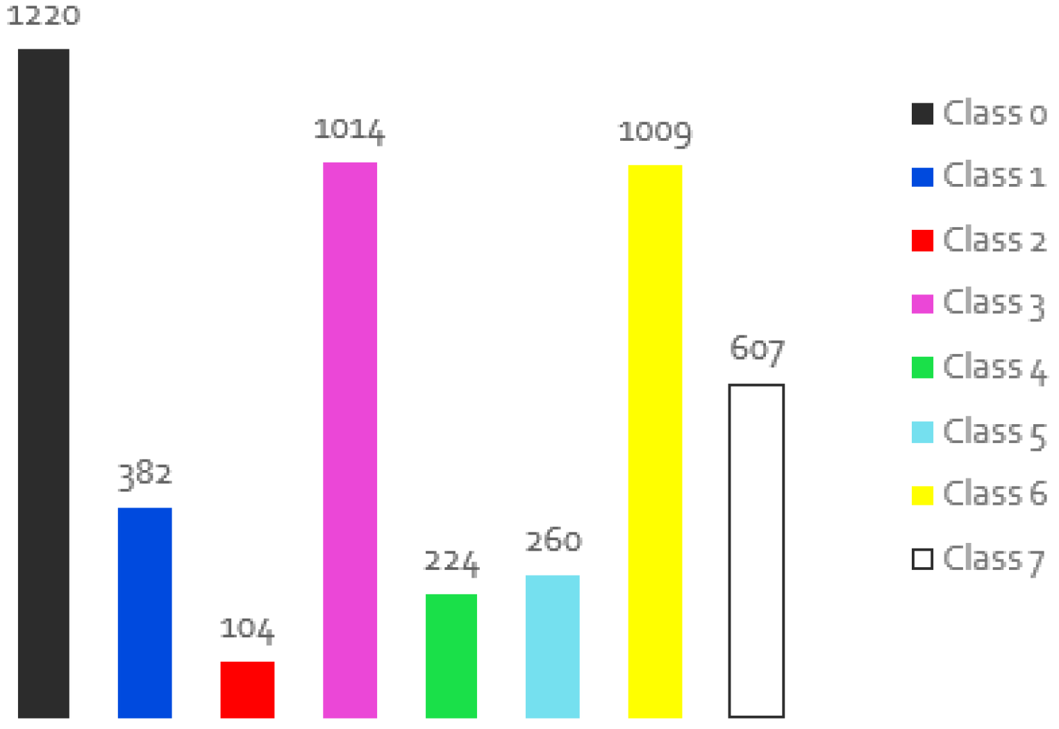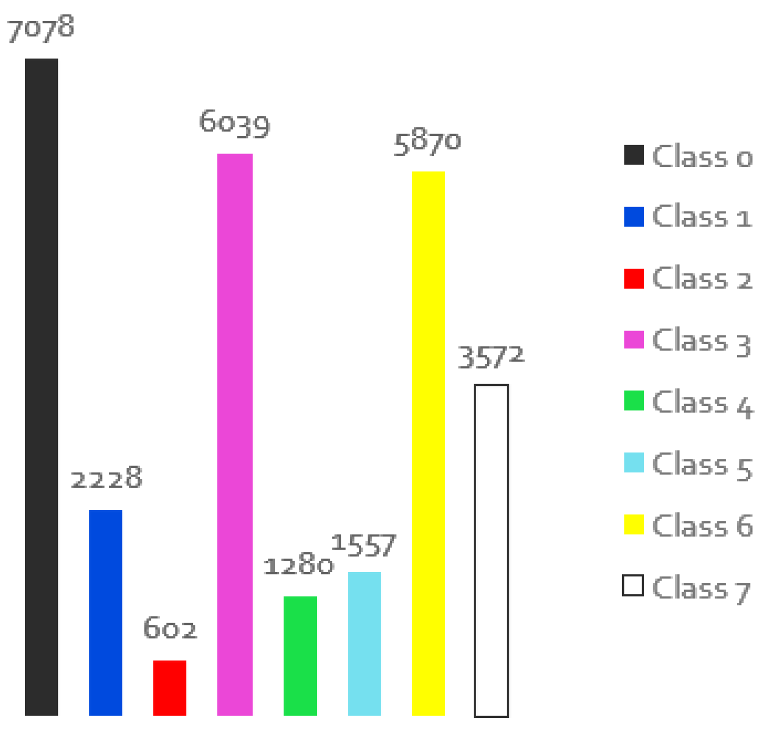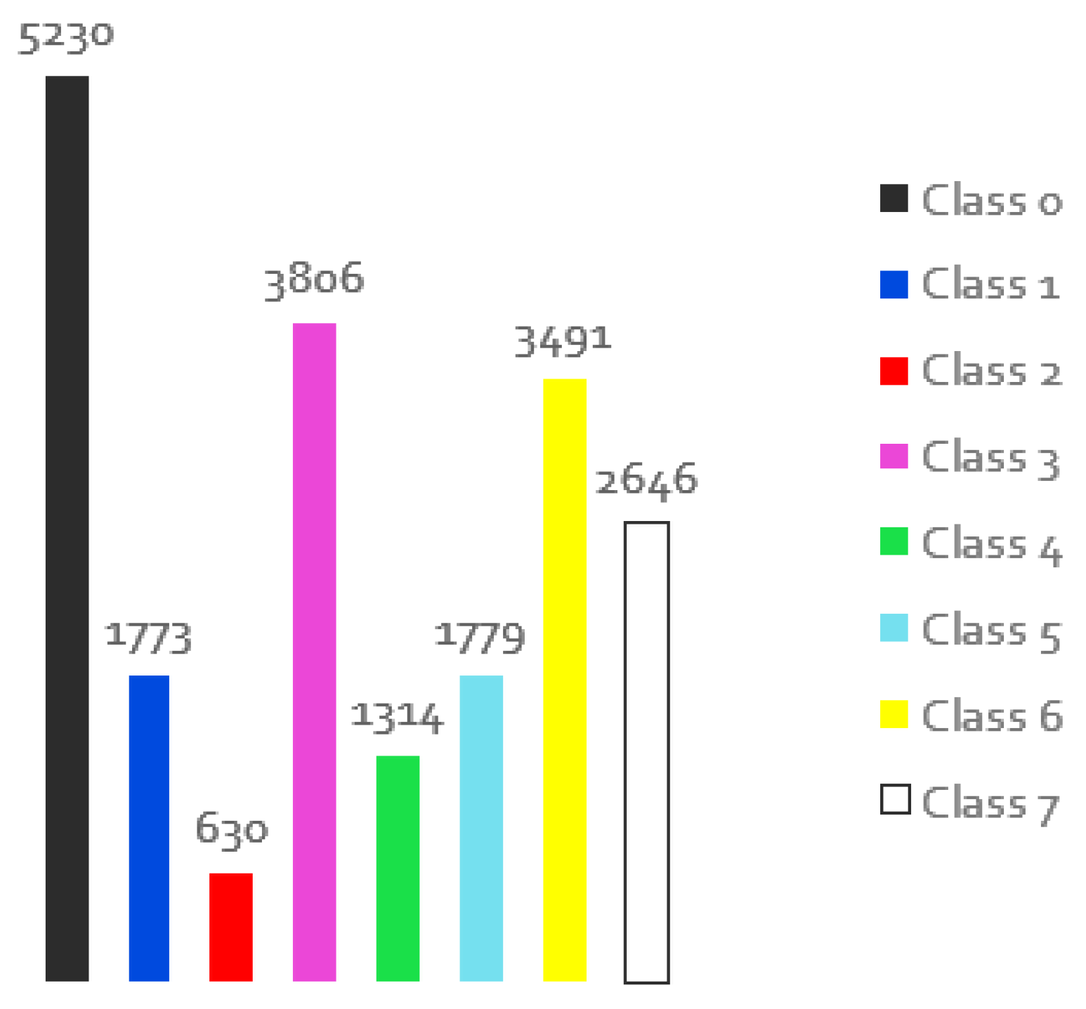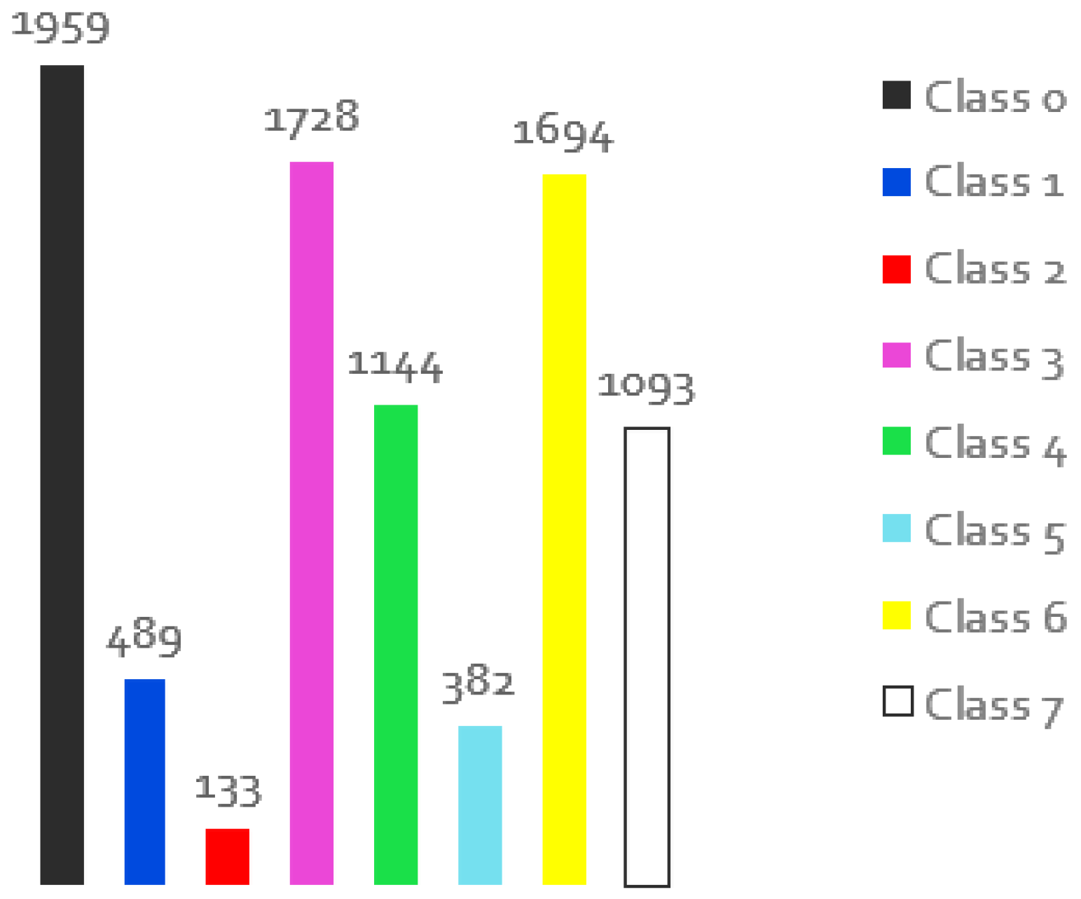Figure 1 shows the representativeness of the classes in the original dataset, i.e. in how many images a class is present, according to the respective colour that appears on the masks.

Therefore, a series of experiments were conducted under different conditions to find out which of SegNet, PSPNET and FCNNs is most suitable for the intended context, and Segnet stands out in the results obtained. This approach is a deep convolutional encoder-decoder architecture for image segmentation that has good segmentation performance in terms of both memory and computation time. It also offers a smaller number of trainable parameters than other approaches. The study carried out on the selected underwater dataset shows a good trade-off between the accuracy of the results and the time required, even though time is not the most important factor. In order to test this type of application, it is important to resort to different techniques to measure the performance obtained after the training. Therefore, in addition to observing the final results, it is generally possible to use the overall and mean accuracy, which refers to the number of pixels correctly assigned (the mean takes into account the predicted classes). It is also possible to calculate the intersection over the union, which calculates the performance of each class taking into account the area of overlap between the prediction and the real observation and the union of the two areas, i.e. the well-predicted and the poorly-predicted pixels.

An example of the final results obtained is presented, where a test is performed on the original dataset with more than 1500 images for training and 110 for evaluation. It is important to point out that the test dataset is hard as it contains the biggest challenges encountered in underwater visual data collection such as: inconsistencies in lighting, boundaries of objects that are not perceived as a whole, etc. The test is performed after every 500 random images, and a total of 100 evaluations are performed to obtain the final model and performance metrics. However, the best model was found after 45000 images, i.e. after 90 evaluations. Table 1 summarises the results in terms of overall accuracy, mean accuracy, mean IoU and the values for this metric for each class.

As can be seen from the table, although the results are generally not bad and useful, there are errors in some classes that are dangerous from the autonomous vehicle’s point of view. For example, the Plant and Robot classes show IoU values of less than 30%, which can lead to some erroneous actions. In the initial experiments, it was found that this can occur because these classes have a smaller number of images for training compared with the rest of classes. 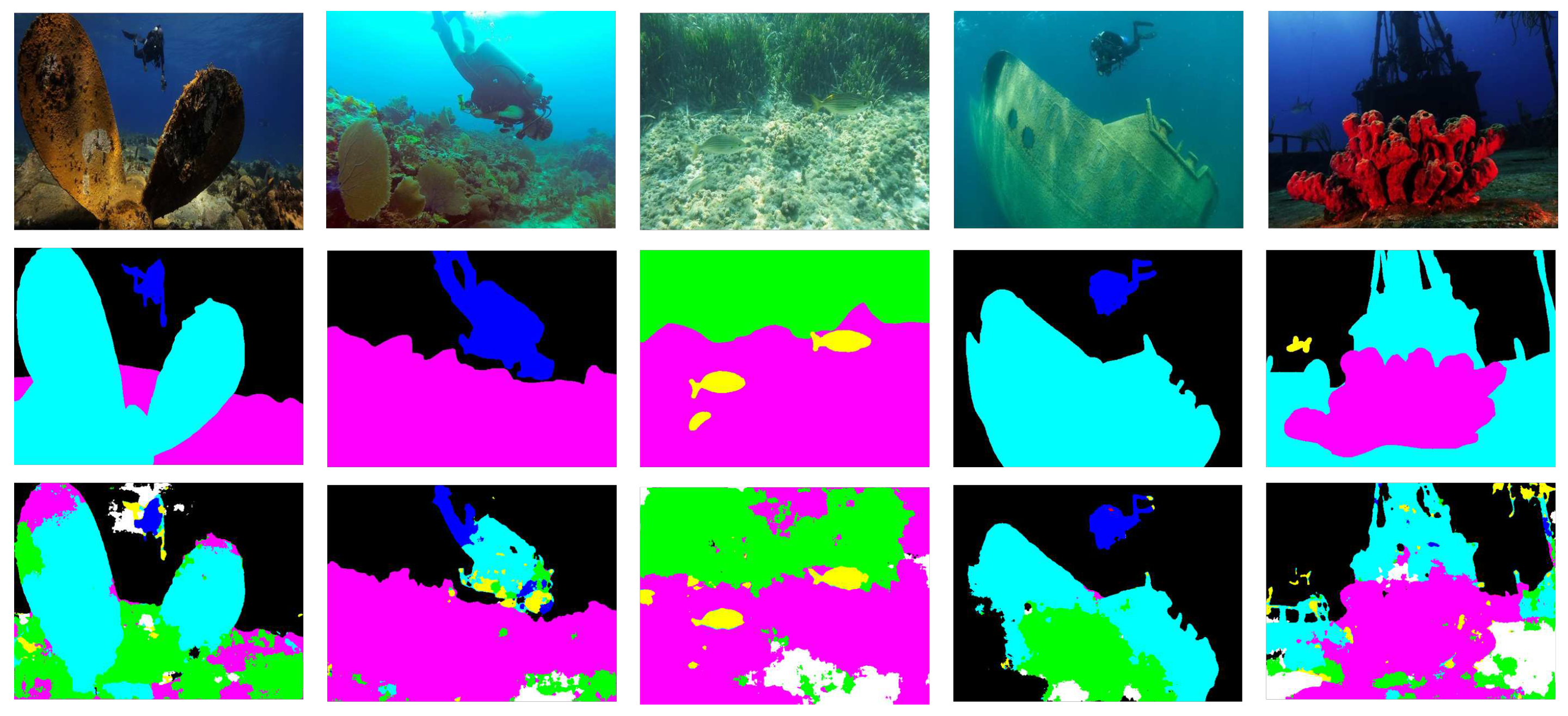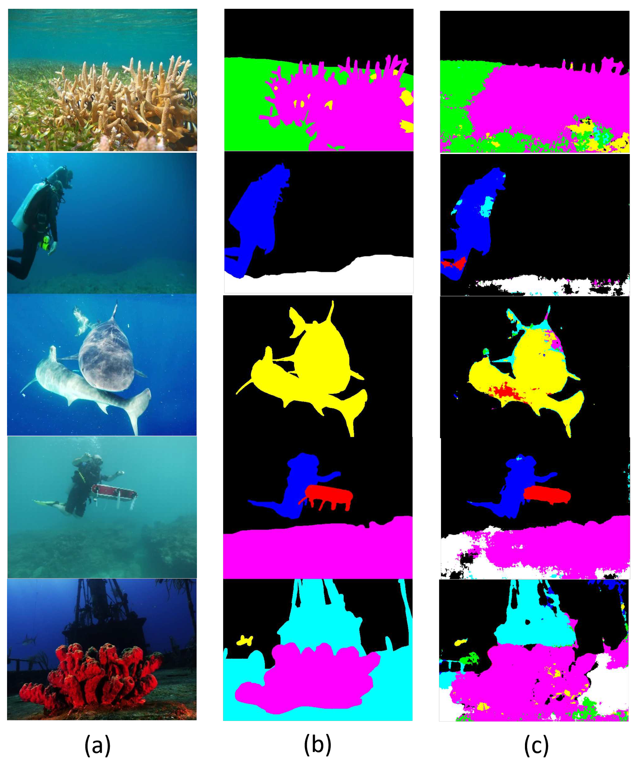In the Figure 2 the results for semantic segmentation for 5 examples can be seen. In general, it was found that the boundaries of the elements are correctly selected, but some of them are assigned to a wrong class, like the diver in the second image or even the wreck in the fourth image.

Although the results obtained are not bad, it is important to investigate if there is a way to increase these numbers to avoid possible errors. Since the investigation of the parameters of the model has already been done, the next steps will be to investigate other strategies to apply in the training dataset. As mentioned earlier, visual data collection in this world is not easy as it is an expensive task that requires appropriate materials and communication platforms and is often dangerous for divers. In addition, this task brings several problems, such as light absorption, turbidity and limited range, which reduces the number of good quality images. The existing datasets for the train of semantic segmentation are therefore intended for out-of-water applications, and when underwater, they are sparse in terms of classes (often a dataset contains only one class, e.g. for fish classification) and has a smaller number of samples (many of them contain 1000/2000 images in total, which is considered a small dataset in the literature). In this particular case, the dataset contains a total of 1525 images for training with 8 different classes, which may mean fewer images per class. Furthermore, this dataset is unbalanced, as the class with the highest representativeness is represented by more than 80% and the class with the lowest representativeness by less than 10%. Another crucial aspect of this dataset for semantic segmentation is the need for proper annotation for the training process, and this task is challenging as it often has to be done by the user or with the help of computer tools, but this takes time and is challenging. The dataset tries to represent each class under different viewing angles, lighting conditions, sizes, etc., as in the case of the fish class, but in some other cases this is difficult. Some of the images have worse visual conditions, with bad boundaries and without correct information about the colour of the objects, and some of them have some discrepancies in the annotation mask (because it is a difficult and repetitive task). In the Figure 3 you can see some of SUIM-dataset problems.

In this way, it is visible an example of pictures with more fish than in the ground truth image because there are difficulties in the annotation, another example is the same class with a different annotation, which can confuse the learning process, and the third example shows the difficulties that often occur when perceiving the boundaries of the objects. Therefore, it is necessary to review the weak points of the dataset and improve some problems and solve others to improve the final performance (e.g. poor segmentation).

3. Auxiliary Techniques for Semantic Segmentation

According to the literature and all that is known about the visual conditions of this underwater environment, there are high expectations of the improvements that the enhancement of visual data will bring to the end results of all processes that need to manipulate underwater images, namely semantic segmentations. According to the current state of the art, there are several techniques for different enhancements. One of them deals with the restoration of true colours, another with filtering techniques to de-noise the image, and others that allow the removal of backscatter caused by tiny particles in the water that reflect light back to the camera [18]. After some research in the literature, it was decided to test three techniques that seemed to be suitable for the intended application: Contrast Limited Adaptive Equalisation (CLAHE) [19], White Balance (WB) [20] and a third technique that came from diving experience and summarises some enhancements suitable for underwater imaging. Thus, in detailed way:

CLAHE is used to increase the contrast of an image by redistributing light across the image. It is one of the methods of histogram equalisation, but it is not applied to the whole image, but only to small areas to reduce noise and provide a method that combines the different tiles without their boundaries being visible. This method is very important in underwater scenarios as there are different lighting variations and in some cases a lot of darkness, and it promises to improve the visibility of object boundaries and some important features. The implementation used is based on the OpenCv library and some parameterisation is required. After some experiments, a higher quality image for the context was found by dividing the images into tiles of 80x80 pixels and using a clip limit of 1.
WB is a process that adjusts all pixel colour information so that it looks natural to humans. This is not an easy task underwater, as water absorbs and scatters light differently than in air, and many colours disappear at depth, where everything looks blue or green.In this context, this technique is used as post-processing, but it is not trivial to achieve the correct white balance. There are several variations for implementing this technique, and the approach used [21] shows that realistic degradation of the colour constant can be accurately minimised without producing unrealistic colours, such as the purple of the grass, which can affect the results of semantic segmentation. However, the approach used was not tested in underwater environments, which is why some images without quality were produced in the experiments. However, different parameter combinations were used and when a pattern of behaviour emerged in the results, the better combination was chosen.
The third method compared in this study, referred to here as dive correction [22], is the result of combining the different filtering methods. It is a tool that can be used in code or with as desktop tool and consists of a philtre that adjusts each colour channel to restore the true colours and make the image appear more natural and contrasty.

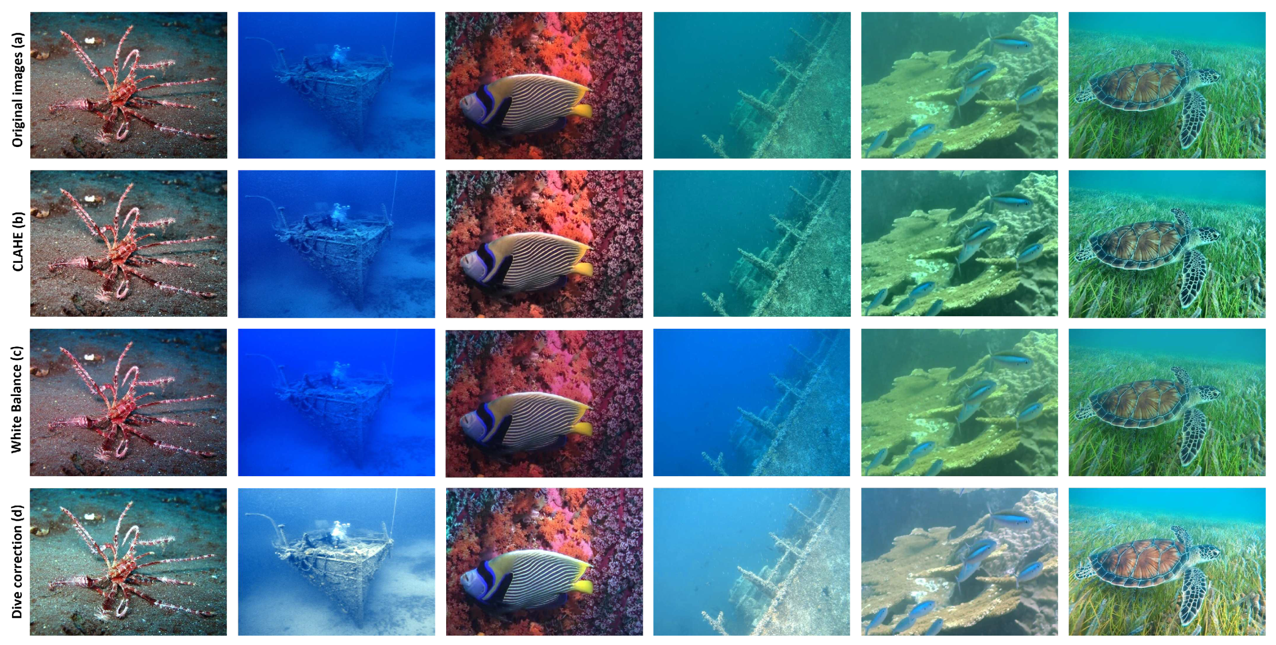
It is also important to mention that since these methods only change the aspect of the image, it is not necessary to make a change in terms of ground truth, and for this reason the original masks were used. The three methods are thus applied to the entire dataset of the training and also the test images. As can be seen in the Figure 4, the results of the enhancement methods vary when compared to each other, and it is therefore necessary to check if this pre-processing improves the final result when applied before training the model. As can be observed, the results vary and lead to images that are more visually appealing with some enhancements, but the same enhancement can lead to undesirable images for other.

Another reason for the poor results of semantic segmentation could be that the dataset is often too small compared to the need, and obtaining labelled datasets is expensive and time-consuming. Therefore, training the models with small datasets is another crucial challenge, and this dataset contains only about 1500 images. Another approach to improve the results is data augmentation, which consists of various techniques that change the appearance of the images, e.g. rotating, zooming, flipping, colour variations, etc. In this way, the dataset can be enlarged, and the resort to data augmentation offers some advantages to deep learning methods, such as improving generalisation, increasing the robustness of the model to different variations of the input, allowing the use of smaller datasets for some needed applications, and avoiding overfitting since the training data is more diverse. It is also worth noting that in most cases this approach is only used for the training dataset, as is the case in this study. In underwater scenarios this is particularly important because, as explained earlier, underwater imagery presents many challenges and the model has to cope with all the changes and variations. Therefore, it was crucial in this context to take into account lighting changes, distortions and perspective changes as the water causes movements of the camera or objects during the shot, as well as additional noise as the conditions for the shooting equipment are often not the best, etc. 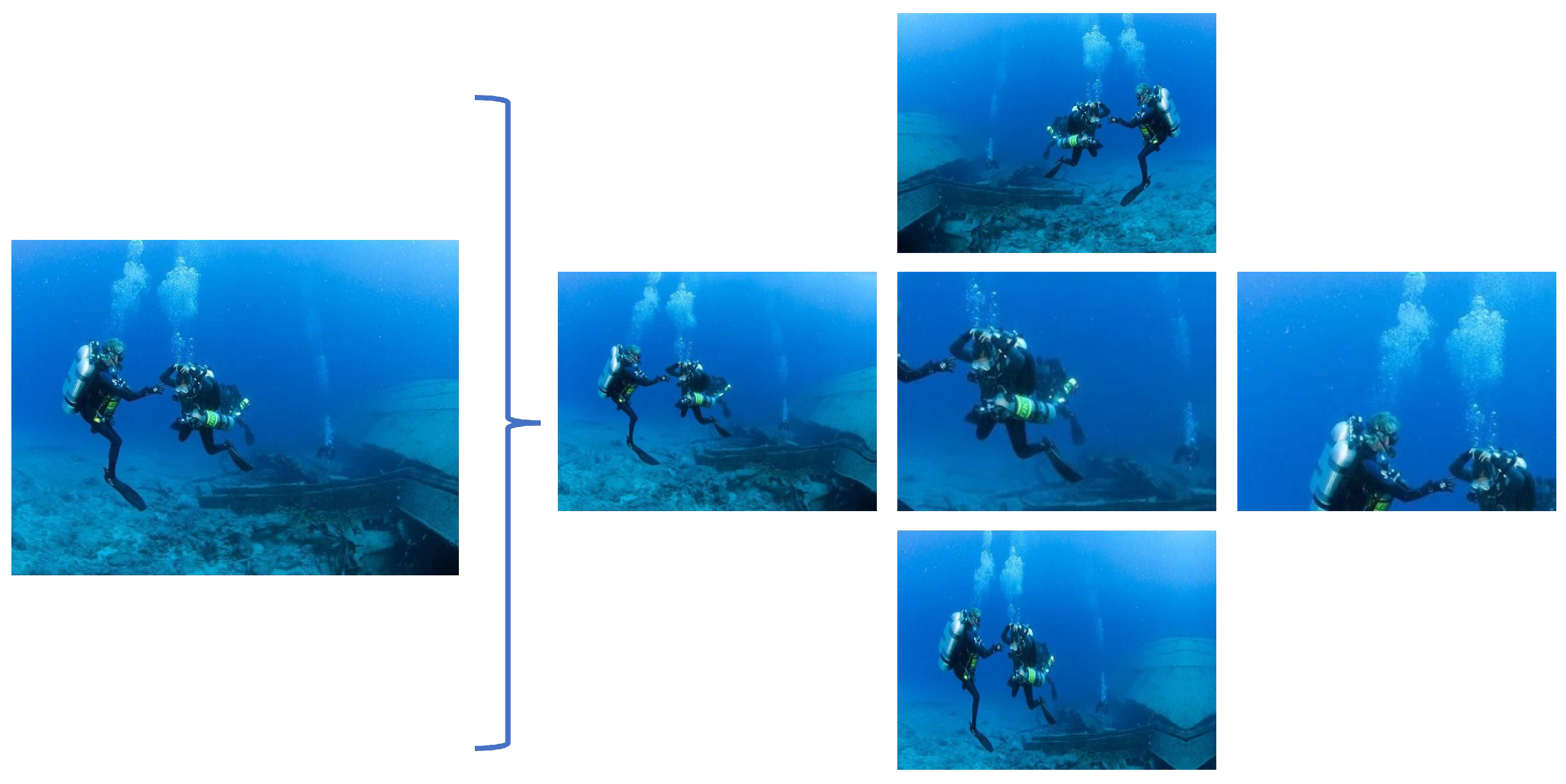Figure 5 shows some of the possible changes that can be made to an image to use it in the training set.

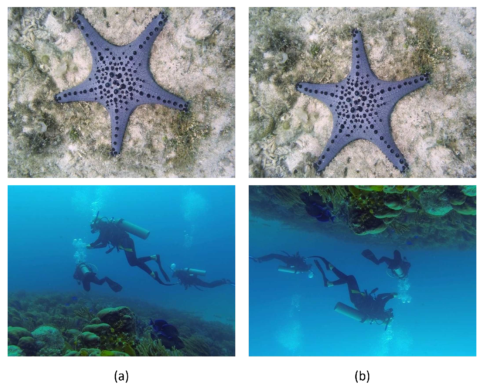
So, in this case, it is possible to get more images with only one image to better train the class of human divers. However, some of these changes are not useful for all scenarios as they change the sense of reality, e.g. when the seaweed appears at the bottom of the image. As can be seen in the Figure 6, vertical flipping is useful in some cases, especially when the camera captures images in an upper plane with respect to the object, i.e. images of bottom of the underwater floor, but it is wrong in cases where the image is captured in front of the object of interest, as can be seen from the air bubbles that can never come down. In many cases, extreme transformations (flipping or rotating) must be avoided.

For this reason, it is important to ensure that this process does not provide misleading information, and for the data augmentation in this application it is assumed that the images are taken from a vehicle that does not rotate much along the x-axis. It is crucial that the consistency of the data provided is maintained, and the changes must represent reality and the greatest possible number of variations in the real world. There are already many methods of data augmentation to increase the size and variety of datasets. However, when a segmented dataset is needed, the transformation must be applied to each image while keeping the ground truth consistent. Sometimes it is non-trivial to maintain this in order not to add false information or, for example, black pixels during the rotation transformation. To solve this problem, it is often necessary to add a crop transformation to the result of the first transformation. But not all transformations require an intervention in the mask, such as the changes in the colour information of the image, where there are no changes in the position or size of the objects. The different transformations can be divided into categories, such as:

Spatial transformations - refer to changes in the image coordinate system that affect the position and orientation of objects and the overall image.
Intensity transformations - change the appearance of objects, but not their shape, and act at the pixel level.
Elastic deformations - can simulate the flexibility of objects, the variability of their shapes or, in underwater scenarios, some water movements that are often seen in the image.
Noise addition - makes the model more robust to the diversity of data collection, especially in underwater scenarios where there is noise in the images.
Random erasing - some techniques remove regions and in the mask this class is ignored.

In the literature there are several implementations of these transformations and libraries for the intended context, such as: ImageDataGenerator from TensorFlow or the transformations from PyTorch, when the user needs to apply the same transformation in the image and in the labelled mask. However, these approaches have some limitations, such as rotating an image and the appearance of black corners. Another option is Albumentations [23], a fast image augmentation library that simultaneously applies the transformations for the images and the ground truth labels and has an extensive set of transformations, from the most common to more unique ones, such as the grid-based distortions, supporting more than sixty transformations in total. It is designed to be adaptable and efficient in applying the transformation to the training process and ensuring that both the image and the corresponding mask receive the same transformations and parameters. It also allows a pipeline of transformations to be put together so that the variety of transformations is incredibly large. 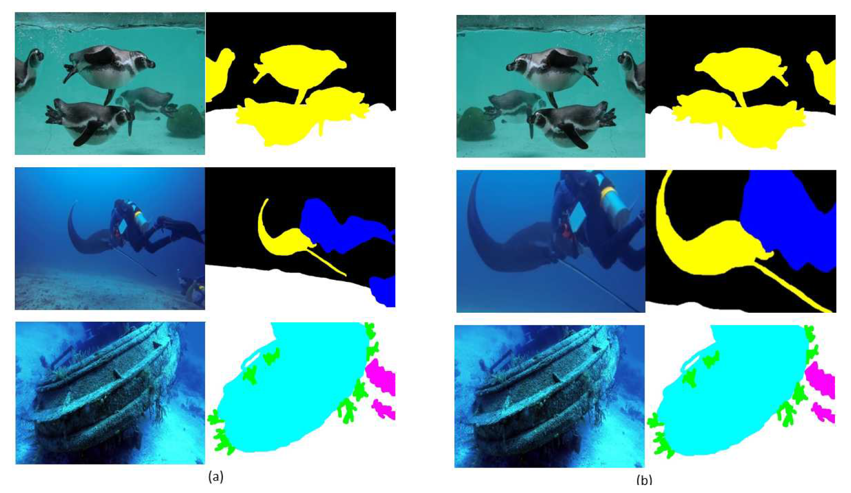For this reason, this library has been used for this work, and in Figure 7 you can see some transformations in the image and ground truth made by this library, e.g. by flipping, cropping and reducing transformations.

4. Experimental Results

In order to be able to verify the statements made in the literature about the selected procedures for increasing the final performance of semantic segmentation, it is necessary to test them individually and analyse their relevance to the intended context. In this way, new datasets are created for each test according to the respective assumptions. To compare the results, the common metrics and the quality of the visual results are used, as explained earlier. All experiments were conducted using an Intel(R)Core(TM) i9-9880 CPU @ 2.3GHz with 32GB RAM computer.

4.1. Enhancement Tecniques Comparison

As described earlier, three implementations of enhancement visual quality of the images are tested and compared: CLAHE, white balance and the dive correction. The corrections are applied to both training images and test images, as they are visual enhancement techniques and the results can benefit from them. For this test, four different datasets were created and the model was trained with a total of 50000 images, with evaluations after 500 randomly selected images, resulting in 100 evaluations each. The results obtained are compared with the original dataset, i.e. with the training performed on images without the image enhancement already described, and can be seen in Table 2.

In general, the mean IoU value is the best way to check the performance of the semantic segmentation methods, since it is calculated with respect to all classes, but since we have 8 classes, it is normal that this value is not much higher. In other words, it indicates how well the segmentation model works across all classes. As for the quantitative results, it shows that the CLAHE has only a small increase in the mean IoU. But it gives better results than the original for tree classes and in the case of the fish class with significant results (more than 3%). For this reason, this enhancement technique seems to be the best, but the visual results should be observed. 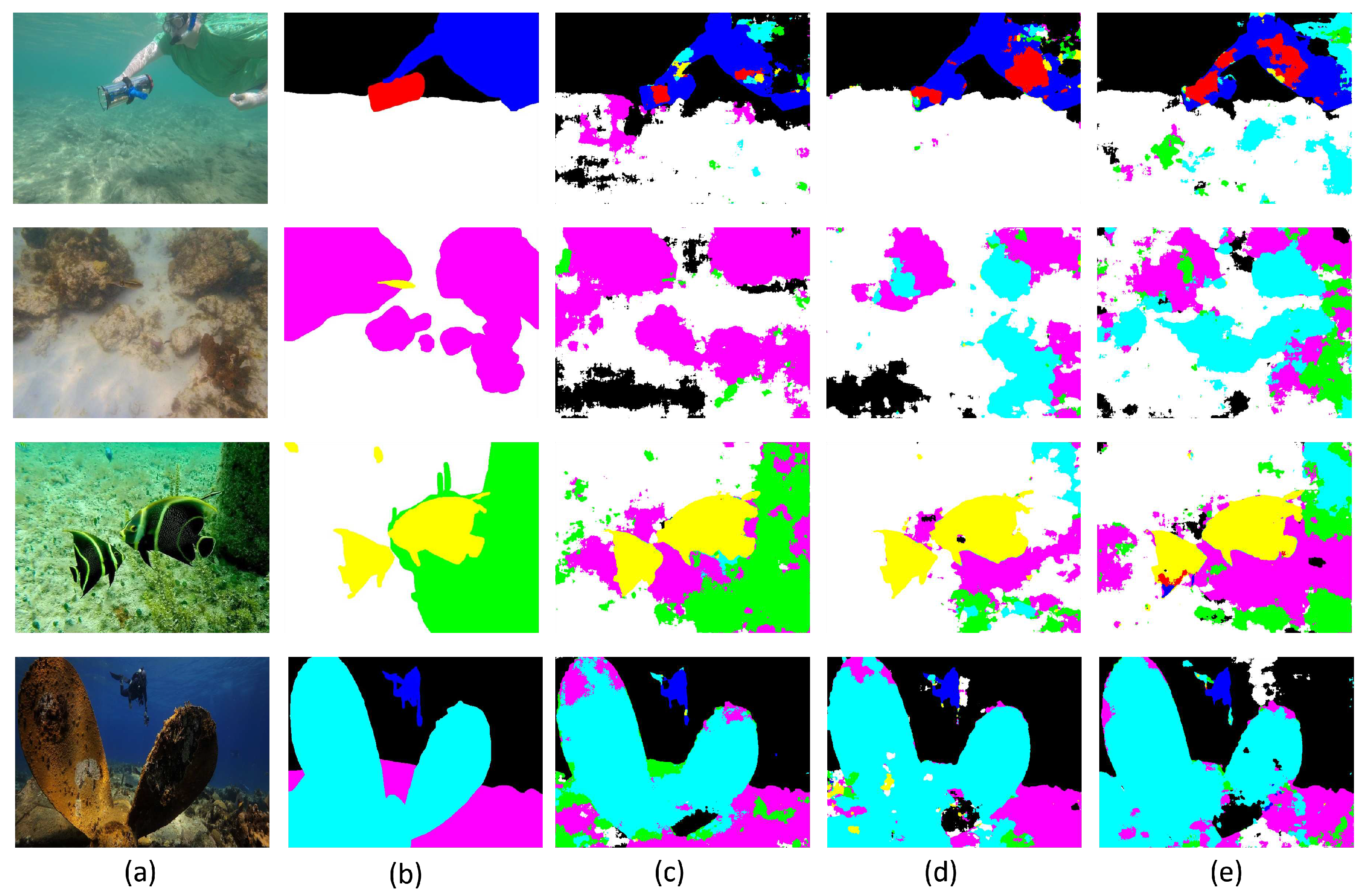Figure 8 shows the results obtained by applying the three enhancement methods to the images.

Looking at the visual results, it is possible that the CLAHE results are generally better because it is the best method to observe the body of the human diver and the coral in the second example. Also, it is a unique method that shows the plants of the third example in a high number of pixels, which is a good result as it is a difficult class to model. The other implementation stands out compared to the CLAHE method in the robot class, but it is not significant because it is only one of eight classes and does not give good segmentation results. In this way, the best result is obtained with the CLAHE method, which slightly improves the final result and has a higher overall accuracy, i.e. a higher rate of well-detected pixels. This result was to be expected, as the contrast and therefore the visibility of the main features of the images is improved, which can increase the performance especially in underwater images with different lighting conditions. It is also important to mention that this enhancement technique allows the model to reach the best value of mean IoU (within 50000) after 90 evaluations, i.e. using a total of 45000 training images instead of 50000 for white balance enhancement or 47500 for dive correction. For this reason, the CLAHE method is chosen as the best and most appropriate for the context and for use in the next experiments, if necessary. 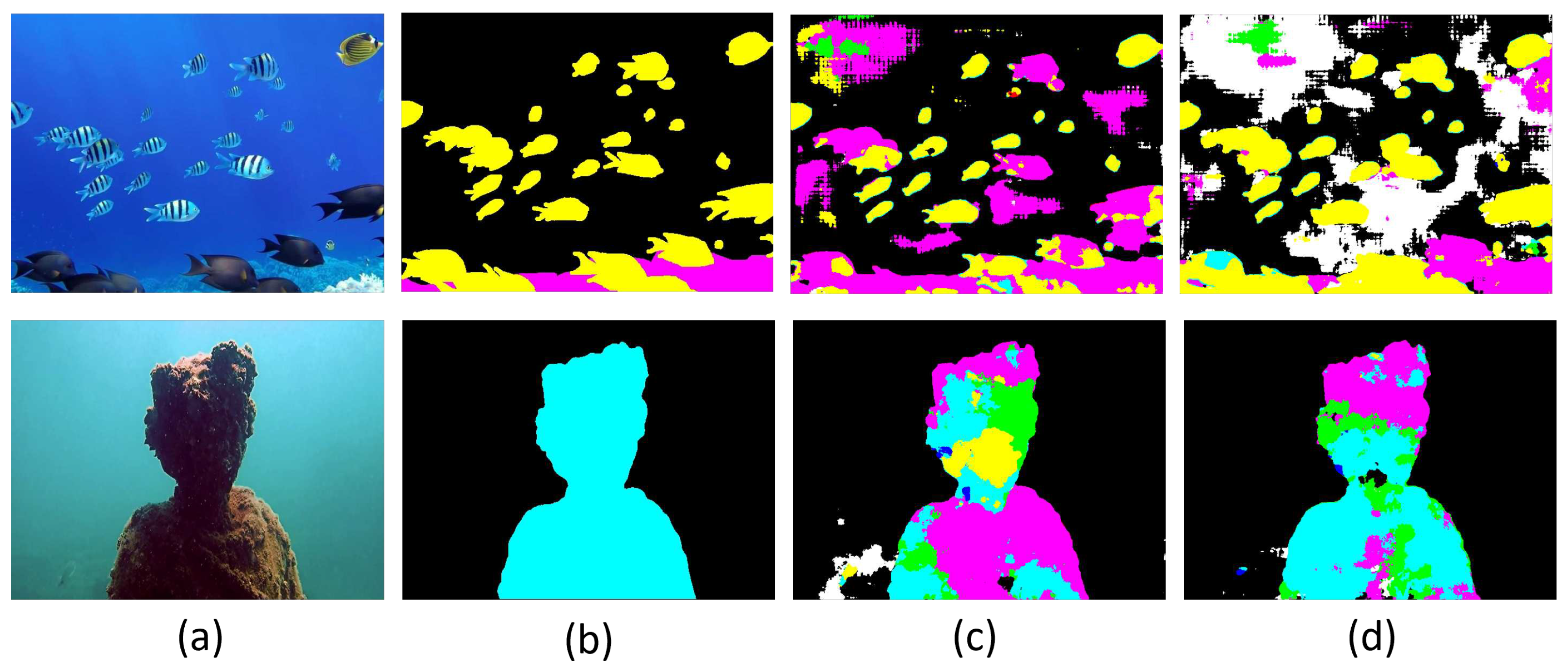Figure 9 shows an example of the improvement in the final segmentation results using the CLAHE method in the fish and wreck classes compared to the original results.

4.2. Data Augmentation Influence

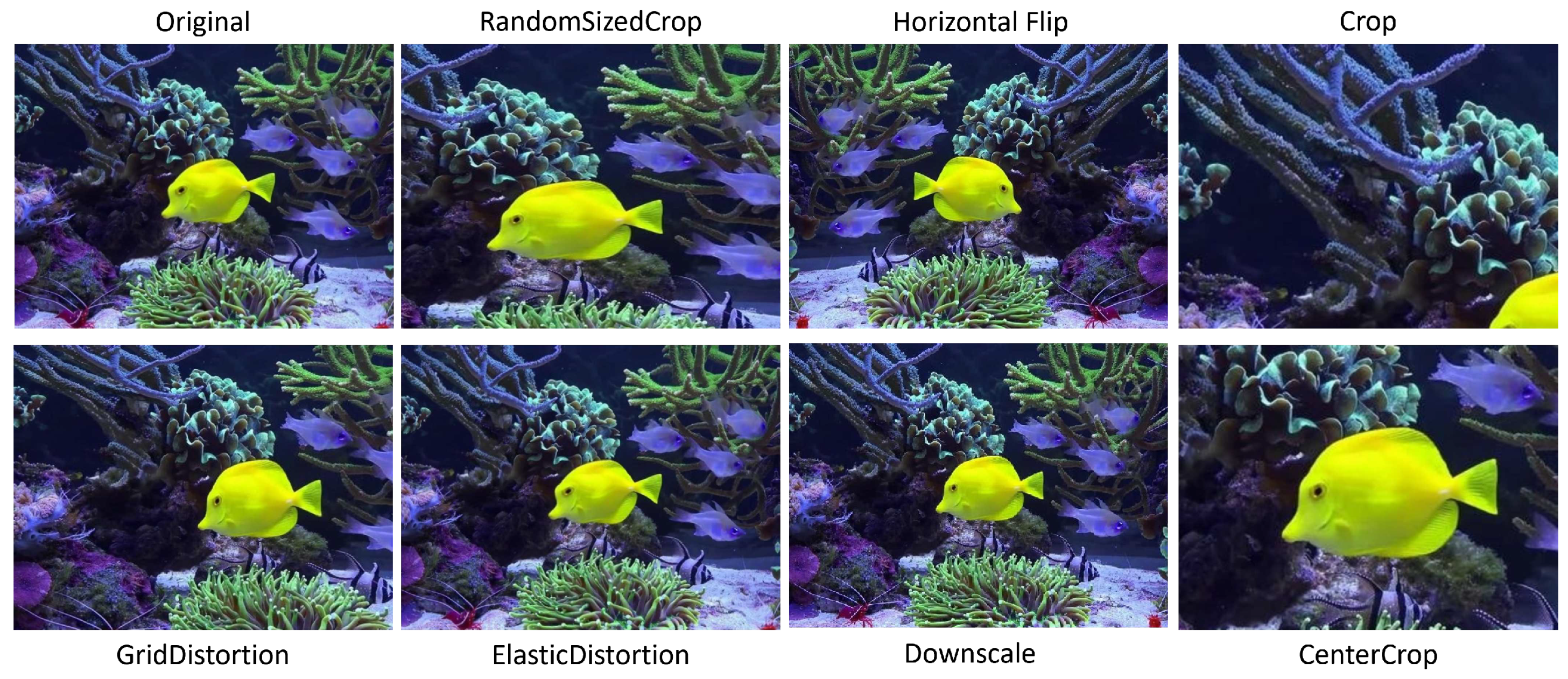
As far as data augmentation is concerned, there are several options that can be applied to the images, but it is not possible to apply all of them because the data set would be larger than the need and the processing time would increase greatly without need. To create the datasets with data augmentation needed for the following tests, a total of eight transformations were used, which can be seen in Figure 10. Clipping operations were used as well as some distortions (grid and elastic) and a flipping in the horizontal axis. It is important to note that the test of the influence of data augmentation was carried out in a isolated way, i.e. without visual enhancement methods.

4.2.1. Geral Data Augmentation

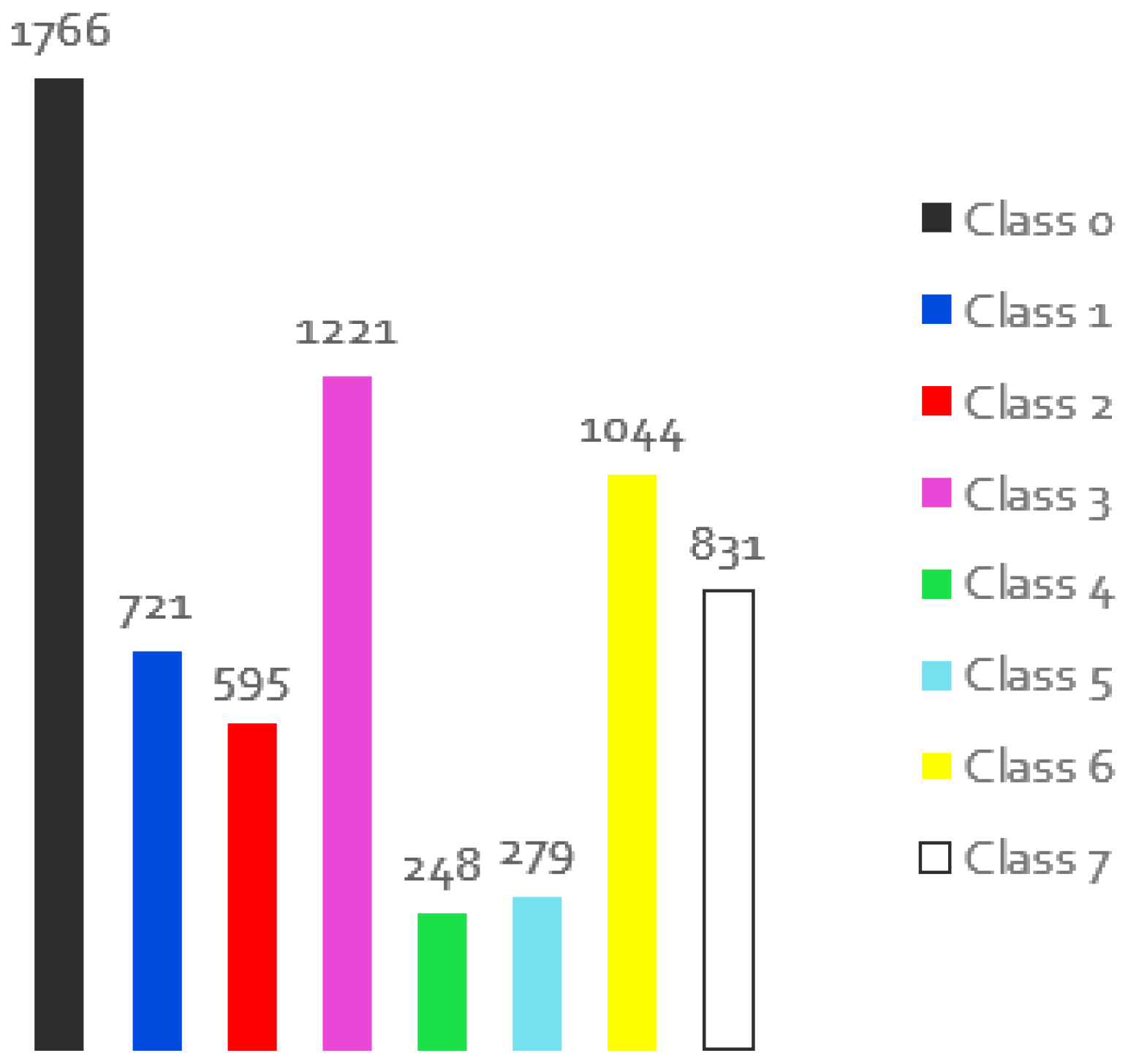
The first experiment with data augmentation was conducted on a dataset where 5 of the augmentations shown were applied to each image in the training dataset. This gave a total number of 9144 images for the training dataset to be able to evaluate the effects of training in a larger dataset, because 1500 images is a small dataset for the intended context. Figure 11 illustrates the distribution of classes across images. It can be seen that the number of samples per class increases and the distribution of classes remains the same. To allow a fair comparison and because the new dataset is larger, the original dataset was run for 50000 training images, with the evaluations done for 1000 images at a time (about two-thirds of the total number of images). Therefore, the new dataset with data augmentation (DA) was run after every 6000 images for a total number of 300000 iterations, aiming to have the same number of evaluations at the end, i.e. 50 evaluations. Table 3 summarises the result for the best iteration for the original dataset and the dataset with data augmentation (iteration 41 and iteration 47 respectively).

Looking at the results, it is possible to see that increasing the number and variety of sample, under equivalent conditions for thre train) increases the general value of the mean IoU by about 2.5%, which is a relevant result because there are 5 classes whose IoU of the results is increased. There are two classes where the behaviour decreases, but one of them is a difficult class to model (plants) and another is a general class because it is rocks and the value of this class is still useful in the intended context. 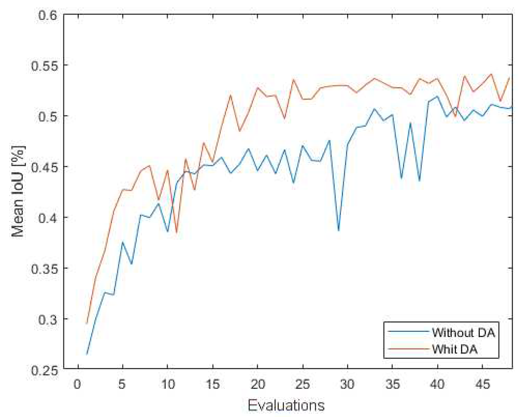Figure 12 shows the results obtained during the learning process in terms of the mean IoU value.

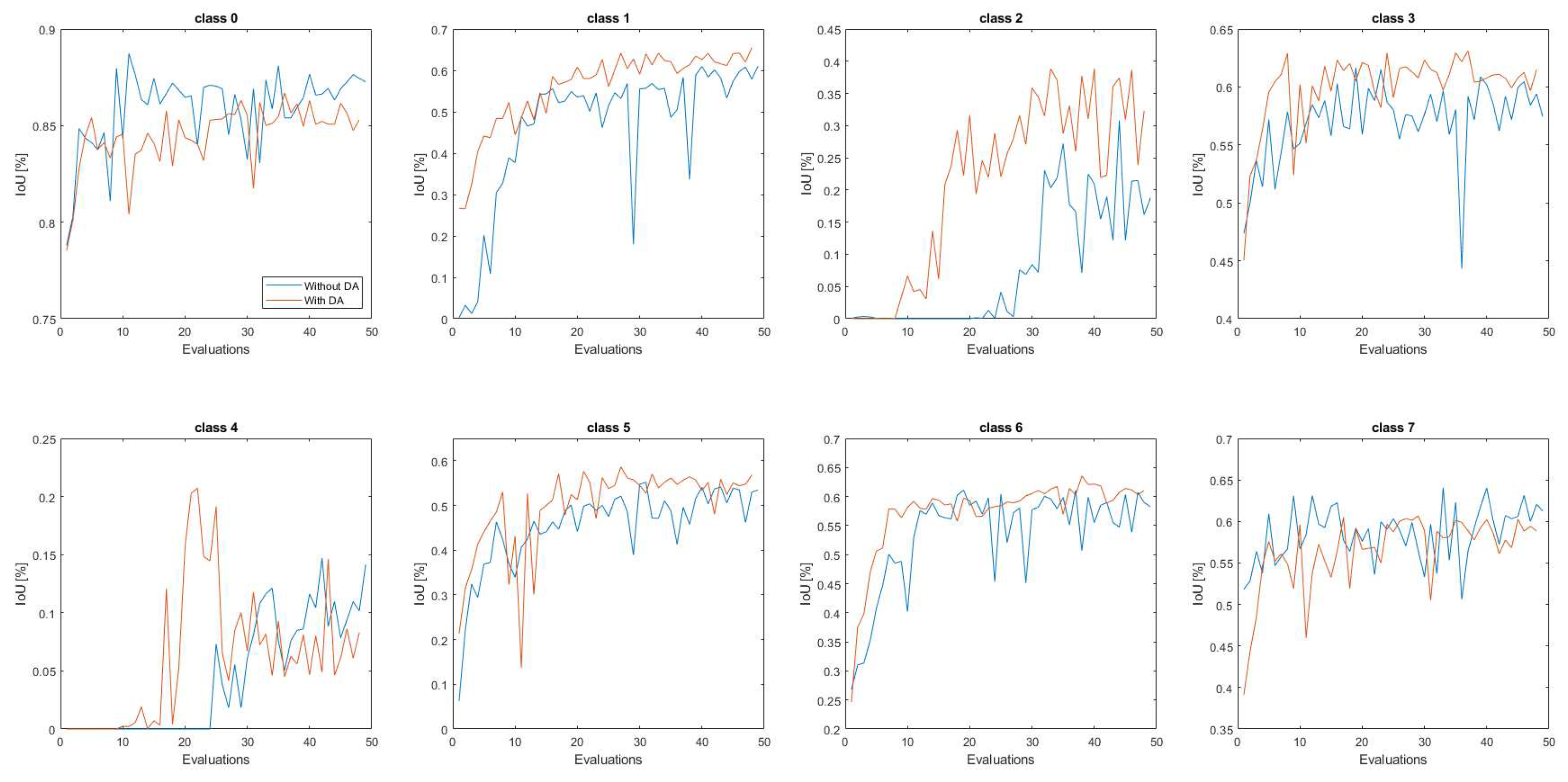
It can be seen that the result with data augmentation generally performs better throughout the process, and if we look at the first 25 evaluations, we see that the difference between the maximum values reached is about 6.5%, which means that the data segmentation learns faster. Figure 13 shows the same analysis, but in relation to the individual classes of the process.

It can be noted that in most cases the data augmentation improves the result of the IoU values or starts better and faster than the results without data augmentation. With respect to classes 0 and 7, the results of DA are not better than the original results, but these are common classes that are strongly represented on many images and for this reason are easy to learn. Regarding the worst classes (plants and robots), it is important to point out that with data augmentation, the results with better performance start earlier, which means that the ability to learn in the training dataset with a larger number of samples. These two values are lower than those of the other classes because the dataset is unbalanced with more images, which means that these classes are less represented than the others.

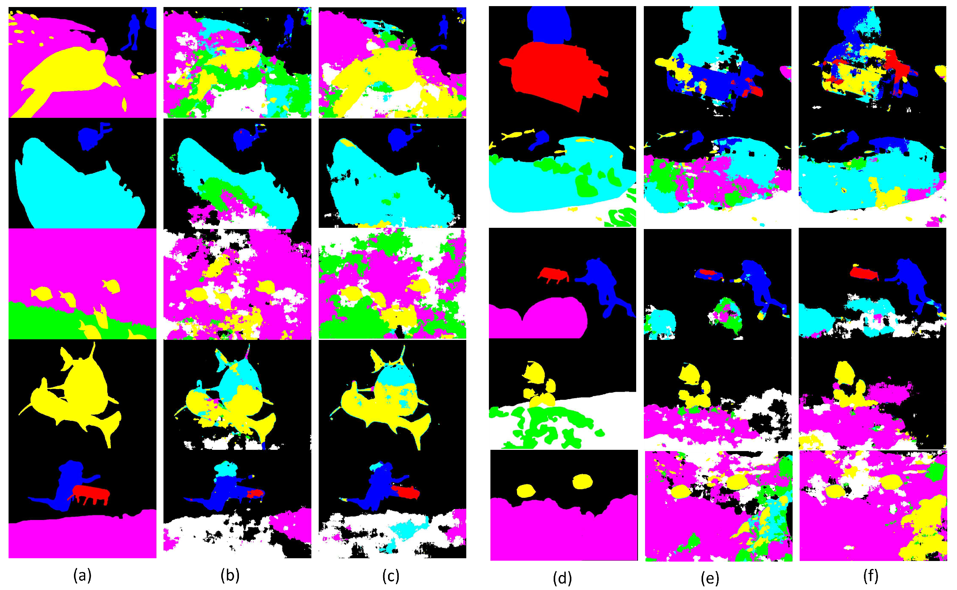
Figure 14 shows the results of the original dataset (second column) and the dataset with augmentation (third column) with the same configurations. It can also be seen that for most classes and images, the result with the augmented data is better than the previous one. Pixels identified as robots occur in large numbers, and wrecks and duman divers are better delineated. Plants and robots are the classes that give the worst results, as they remain the classes with low representativeness.

4.2.2. Data Augmentation of the Less Representative Classes

Now that it is clear that segmentation is well suited to improve the results, as it produces more images in which the classes are represented with different perspectives, sizes and image qualities, the next experiment is to see what happens when we apply data augmentation to all images, but in a different number of variations according to class.

Looking at the distribution of the original dataset used for training (see Figure 1), we can see that the classes robots, plants and wrecks are less represented in the images. Therefore, 2 image data augmentations (RandomSizedCrop and HorizontalFlipping) were applied in all classes and another 5 transformations (CenterCrop, Crop on the left, Grid and Elastic Distortion and Dowscale) were applied in the less representative classes (classes 2, 4 and 5). The generated dataset includes a total of 7312 images, which is a larger dataset, but it needs to be verified if this number of images is sufficient to model the 8 classes. The new distribution of classes in all images is shown in Figure 15.

It can be seen that the less representative classes are the same as in the previous experiment, but with higher number of samples per class. The higher representative class is present in about 70% instead of 80% of the images and the three less representative classes are present on average in about 17% instead of 12%. It should be noted, however, that the increase in the worst class is not proportional (while the robot class increases by 6 times, the wrecks increase by 7 times) because the classes are not isolated in the image and some cropping transformations may suppress some of them. This factor in addition with the different size of the representation of each class in each image may affect this result. In the same way as in the previous experiment, training was performed on the images of this new dataset with data augmentation (DA1) after every 5000 images (about two-thirds of the total number of images in this dataset) for a total number of 250000 iterations, with the aim of obtaining the same number of evaluations at the end as the original result presented before. Table 4 summarises the result for the best iteration for the original dataset and for the dataset with the new data augmentation dataset during the segmentation process over the 50 evaluations.

As can be seen, the value of the mean IoU as well as the mean Acc increases because there are some classes that increase both the accuracy in detecting the pixels and the ratio between the area overlap between the prediction and the mask with the union of the two. The classes that are more augmented in the training set increase the value obtained, except for the wrecks, but the value is similar to the original one (less than 1%). However, the plants and the robots increase the value of IoU by 12% and 16% respectively, which is good because they are difficult to model and learn. The class of divers is not highly augmented compared to the robots, but they increase their IoU value because in most cases the robots appear on the image together with the human divers. The wrecks (class 5) do not improve their results even though they belong to the augmented classes, but their results are already higher than 50% and for this reason it is a good result. A curiosity is that this model was selected because it has the best value for the mean IoU during the 250000 training iterations, but this best value corresponds to iteration number 22, i.e. much less evaluations until the best performance. 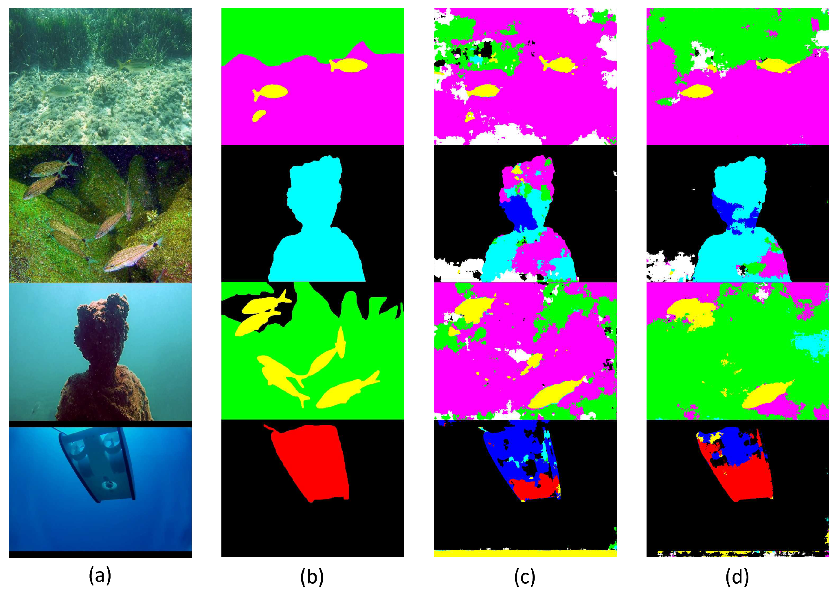Figure 16 therefore shows the segmentation obtained for images with the classes that are augmented in the training process: Wrecks, Plants and Robots, and for these particular cases one can see that the results are much better than those obtained with the original set. So you can see that the results are better with the data augmentation because the area of the plants is much better delineated and the bodies of the robots and the wrecks are well identified in terms of class even with more pixels.

4.2.3. Data Augmentation of the Isolate Classes

The last result related to data augmentation has the main objective to test if it is possible to increase the value of an isolated class by data augmentation in the images when this class appears. For this purpose, a dataset was created in which the images of the robot (class with low representativeness) were augmented with the 7 semantic segmentations of those previously described. The new dataset shows the distribution of the graph of Figure 17, obtaining a total of 2252 images.

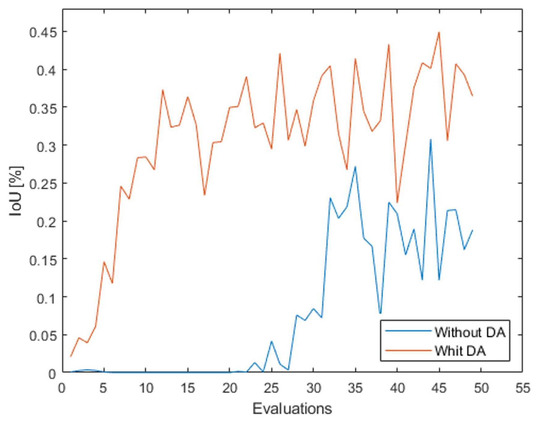
The number of images with the robot class increases sharply and its representation reaches more than 25%, which is a good result for a dataset with 8 classes to be segmented. The plant class is the class with the lowest representation and the human divers increase their value to more than 30% as they often co-occur with the robot. Therefore, this dataset was trained with a total of 75000 images, evaluating all 1500 images to perform a total of 50 evaluations, and the best model was determined after 36 evaluations. The result of this best evaluation gave an IoU value of 41.4% for the robot class, which is an incredible result for the class that had a maximum value of 20.9% in the original case. As expected, the value for the human diver increases to 67.8%, and these two increases lead to a higher mean value than in the original case (54.5% instead of 51.8%), proving that when working with different classes, one or two of which give poor results, the final value of the mean IoU can be sacrificed a lot. In Figure 18 the result for the value of the IoU of the robot class can be seen throughout the training process.

It can be observed that in addition to the fact that the value in the original dataset is always lower than when the images with data augmentation were used for the robot, the values in the data augmentation dataset start to show before. In the original case, the class shows results higher than 0 (also unusable) after 25 evaluations.

Figure 19 shows the result of some images with robot class present, for which the best model obtained in this test was used.

In the same way, the class plant is another one that is less representative in the original set, and so a dataset was created in which the images of the plant were augmented using for that 7 semantic segmentations. The difference is that only about 100 of the total number of plants are augmented, because this class occurs in many images with very small sizes or only in one corner of the image, and the transformation produces images without this class (see Figure 20). The remaining images are retained in the dataset without data augmentation in a similar way as all images without plant class.

In this way a dataset is obtained with a total number of 2588 images, but with more images with the plant classes, this class being the fourth class most represented in all the images, see Figure 21.

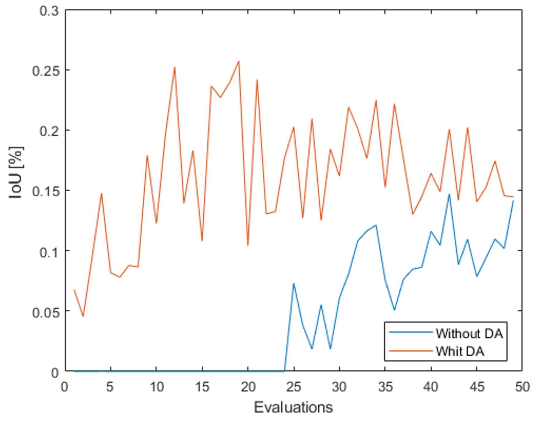
Therefore, this dataset was trained with a total of 75000 images, evaluating all 1500 images to perform a total of 50 evaluations, and the best model was obtained after 45 evaluations. As for the result, a similar behaviour as for the robot class can be observed, i.e. starting with values higher than 0% and obtaining higher results over the 50 evaluations (see Figure 22), with the best model obtained with a mean IoU of 53%. In this case, however, the best value of the mean IoU does not refer to the best value of the IoU for the plants, as all classes are considered in this metric. The value obtained for the IoU for the plant is about 20% for the best value for the semantic model, which is also a higher value than the results obtained without data augmentation. It is important to point out that this class is very difficult to model because it can appear on the image in different sizes, perspectives and variations.

4.3. Data Augmentation with CLAHE Method

In order to evaluate the effect of using both strategies simultaneously and to see if the results improved, it was decided to use the DA1 dataset, i.e. the more balanced dataset of the previous tests, where the less representative classes were supplemented with new image samples, and the better ehancement technique (CLAHE). Therefore, training with the images of this new dataset (DA _C)) was performed after every 5000 images for a total number of 250000 iterations to make 50 evaluations. Table 5 shows the comparison between the new results and the results obtained in the test with the data augmentation only. In this way it can be clarified whether it makes sense to use both or whether the data augmentation is sufficient.

From the results we can see that all general performance metrics are increasing, especially overall accuracy, which has been the best metric since the first test, i.e. pixels that belong to a class according to the model are that class. Mean Acc algthout with less result, considering not only the amount of pixels well assigned but also the class of each pixel, exceeds 1.5% and in terms of mean IoU it was the best result ever obtained with this dataset, reaching 56%, which is a good result considering the number of evaluations that are performed. Looking at the results of the individual classes, we can see that they are all increasing, except for the value of the plants. It is important to mention that the value of IoU obtained during the training process for the plant class has a maximum of 17.3%, but in the table the values considered are those obtained for the best value of mean IoU during the training process, considering all classes at the same time. This may be because the CLAHE could damage the region of the specific plant areas on the images. So, it was proved that both strategies together are a good plan to improve the results in general.

Figure 23 shows the result of the segmented images for some of the images used to test the different approaches with the best model trained on this final dataset, and the results show good segmentations and many of the pixels are well labelled (some of the classes, such as robots of fish, represent the complete object).

5. Conclusions

The main objective of this work was to evaluate whether there are approaches commonly used in outdoor environments that can be applied in visual segmentation methods for the underwater context, and if so, how much they could improve the overall performance of this task. It was intended to find out how to build a more balanced dataset without requiring effort in data collection, which is already challenging and expensive in terms of time and cost, in order to extend these methods to different domains and application tasks. To do this, we start from the findings obtained in a previous study by the authors. In that work, 4 literature implementations for semantic segmented applications were tested and Segnet stands out for its performance and for this reason this method is used in this work. The lack of good datasets to test these applications is still a problem, namely datasets for semantic segmentation that it also requires the labelled ground truth for each image. So, the SUIM-dataset is selected and although it includes only 1500 images for the train, it presents different perspectives, sizes and conditions of 8 classes that are commonly encountered in this world. Although not all objects intended for our applications are covered yet and there are some errors in the labelled masks, in both papers the authors resort to this dataset to perform the evaluations. Therefore, using the Segnet in a training with 50000 training images and evaluations after every 500 images, an overall accuracy of 80%, a mean accuracy of 64% and a mean IoU of 52% is obtained for the best result during these 100 evaluations, which is our starting point: the model shows lower performance, with only three of the total classes achieving more than 60% and two classes achieving less than 30%, which could be dangerous in a real mission. Therefore, some strategies need to be tested to see if it is possible to improve these results, and for that approaches to improve image quality and data augmentation are being tested. The main conclusions regarding the results are therefore the following:

The first test was carried out on 50000 training images, with evaluation after 500 randomly selected images, i.e. after 100 evaluations, with the main aim of finding out which enhancement techniques can improve segmentation performance. The images used for the test are 100, which were selected beforehand and are the same for all tests. Looking at the quantitative results, we can see that the CLAHE method is the only one that increases the mean IoU value, but with a small increase. In terms of the individual classes, this implementation improves the result of corals, wrecks and fish classes. The visual results confirm the quantitative results and for this reason this method was chosen as the best for improving the image quality, as it improves the visibility of the object boundaries and some important features that allow a better training of the model.

The next tests have the main objective to test the influence of the data augmentation for the intended application, since the dataset used is small and a total of 8 transformations were used to create the new datasets used in the tests.

In the first test of data augmentation, a new dataset with a total of approximately 9000 images is created using 5 random data augmentations. The dataset is used along a training of a total of 300000 training images, evaluated after every 6000 images (two thirds of the total dataset) and a new test of the original images is performed over the same conditions (a total of 50000 training iterations and evaluations after every 1000 images to also obtain a total of 50 evaluations). The results with the dataset using the data augmentation increase the original result of the mean IoU by 2.3%, which shows that it is relevant and allows learning some classes with a greater diversification. There are 5 classes that improve their results, namely classes that are more difficult to learn, such as the robot, because it is a class with fewer images in the original dataset (only 104 images), which increases its metric in 17%. However, this class and the plants are the worst classes because the increase in the number of images per class is the same for each class, which also leads to an unbalanced dataset. The classes that decrease its performance decrease by values that are still good and useful in a real context, i.e. they are not dangerous.
The following test wants to see what happens when we augmented the classes with less representative and for this, the images where there are plants, robots and wrecks are augmented with 7 transformations and the rest of them with only 2. However, it is impossible to isolate classes and sometimes when we augment a class with an image, we augment more than this class because in the original there is not only one class. This results in a slightly more balanced dataset where the higher representative class is present in about 70% instead of 80% of the images and the three less representative classes are present on average in about 17% instead of 12%. Under the same conditions as the previous test, the performance for the mean IoU is 54.4%, with robots improving their score and plants presenting a IoU value of 23.5% for the best model obtained during training.
To test whether it is possible to increase the value of the isolated classes, two tests are performed: one with the robot class that is least representative in the original dataset, and another with the plants that are shown to be the most difficult class to learn. For this, the images in which the robot class appears are isolated and 7 transformations are applied and so, the robot is no longer the less representative class. The value of IoU for this class increases for values of 41.4% (value never obtained for this class). When examining the plants, in addition to isolating the images of the plant class, it is necessary to select only some of them to data augmentation, because in many images the class appears with few pixels and the transformations are images without the class. Comparing the results of the class with this data augmentation and the original case, we can see that in test of data augmentation the class presents values higher than 0% first before than than with original case. The values obtained are always higher than in the original test and reach a maximum of 25%. This lower value can be explained by the fact that the images are not very representative with different variations and for this reason it is a more difficult class to learn. These tests show that it is possible to increase the values of a class by feeding the model with a variety of images.
The last test has the main objective to see if the data augmentation and enhancement technique gives good results. For this purpose, the CLAHE method was applied to the data augmentation of the less representative classes (DA1). The results obtained are very good, with a mean IoU value of 56% and an increased Overall Accuracy value of 81.8% (the highest value at this time). The mean Accuracy value is also increasing, which means that the results are better in different classes. The results are better than just applying the data augmentation for all classes except plants, which may mean that the enhancement can confuse the model in the regions of the images (put many saliency features, for example) where there are plants and this class continues to be the most difficult in learning process, but in the visual results this class already appears more.

Considering the last result with both strategies, we can conclude that all the changes made during the study are beneficial and that the results at this moment are better than in the original cases, because now there are 5 classes with more than 60% and only one with less than 30% for the IoU value, and therefore it is a more reliable result and can be more easily used in real contexts. It is important to mention that the results are different from the original results trained along a higher train, which is a good result as it is expected that in longer trains, the values of some classes can achieve higher performance as they are more difficult to train. So, both strategies shows real relevance in semantic segmentation context namely in underwater, where it is so difficult to acquire images with relevance in the quantity need to feed the deep learning techniques.

In terms of future work, the intention is to automate the process of data augmentation to apply more transformations without worrying about the capture this implies, namely, for example, in the rotational or flipping transformations (which are allowed in some cases and avoided in others when it is not practical), and to test the performance with images captured in real missions of the robots. In addition, other objects that are crucial for the movement of the vehicles, such as pipelines, anchors, etc., will also be included in this dataset.

Author Contributions

Conceptualization, A.N. and A.M.; Methodology, A.N.; Validation, A.N; Writing (original draft preparation), A.N; Writing Review and editing), A.N and A.M.; Supervision, A.M.. All authors have read and agreed to the published version of the manuscript.

Funding

This research is financed by FCT - Fundação para a Ciência e a Tecnologia - and by FSE - Fundo Social Europeu through of the Norte 2020 – Programa Operacional Regional do Norte - through of the doctoral scholarship SFRH/BD/146461/2019.

Data Availability Statement

Data available on request due to restrictions eg privacy or ethical

Acknowledgments

The authors would like to acknowledge Minnesota Interactive Robotics and Vision Laboratory for providing the SUIM Dataset [11] that supports this research.

Conflicts of Interest

The authors declare no conflict of interest.

Abbreviations

The following abbreviations are used in this manuscript:

CLAHE	Contrast Limited Adaptive Histogram Equalization
DA	Data Augmentation
FCNN	Fully Convolutional Networks
IoU	Intersection-over-Union
PSPNet	Pyramid Scene Parsing Network
SUIM	Segmentation of Underwater IMagery
WB	White Balance

References

Chen, W.; He, C.; Ji, C.; Zhang, M.; Chen, S. An improved K-means algorithm for underwater image background segmentation. Multimedia Tools and Applications 2021, 80, 21059–21083. [Google Scholar] [CrossRef]
Garcia-Garcia, A.; Orts-Escolano, S.; Oprea, S.; Villena-Martinez, V.; Rodríguez, J.G. A Review on Deep Learning Techniques Applied to Semantic Segmentation. CoRR 1704, abs/1704.06857. [Google Scholar] [CrossRef]
Zhou, Y.; Wang, J.; Li, B.; Meng, Q.; Rocco, E.; Saiani, A. Underwater Scene Segmentation by Deep Neural Network. 2 nd UK-RAS ROBOTICS AND AUTONOMOUS SYSTEMS CONFERENCE; , 2019; pp. 44–47. [CrossRef]
Drews-Jr, P.; Souza, I.; Maurell, I.; Protas, E.; Botelho, S. Underwater image segmentation in the wild using deep learning. Journal of the Brazilian Computer Society 2021, 27. [Google Scholar] [CrossRef]
Wang, J.; He, X.; Shao, F.; Lu, G.; Hu, R.; Jiang, Q. Semantic segmentation method of underwater images based on encoderdecoder architecture. PLoS ONE 2022, 17. [Google Scholar] [CrossRef]
Garcia-D’Urso, N.; Galán Cuenca, A.; Pérez-Sánchez, P.; Climent i Pérez, P.; Guilló, A.; Azorin-Lopez, J.; Saval-Calvo, M.; Guillén-Nieto, J.; Soler-Capdepón, G. The DeepFish computer vision dataset for fish instance segmentation, classification, and size estimation. Scientific Data 2022, 9, 287. [Google Scholar] [CrossRef]
Saleh, A.; Laradji, I.; Konovalov, D.; Bradley, M.; Vázquez, D.; Sheaves, M. A Realistic Fish-Habitat Dataset to Evaluate Algorithms for Underwater Visual Analysis. Scientific Reports 2020. [Google Scholar] [CrossRef] [PubMed]
Beijbom, O.; Edmunds, P.; Kline, D.; Mitchell, B.; Kriegman, D. Automated Annotation of Coral Reef Survey Images. Proceedings / CVPR, IEEE Computer Society Conference on Computer Vision and Pattern Recognition. IEEE Computer Society Conference on Computer Vision and Pattern Recognition, 2012, pp. 1170–1177. [CrossRef]
Alonso, I.; Yuval, M.; Eyal, G.; Treibitz, T.; Murillo, A.C. CoralSeg: Learning Coral Segmentation from Sparse Annotations. Journal of Field Robotics, 2019. [CrossRef]
Fabbri, C.; Islam, M.J.; Sattar, J. Enhancing Underwater Imagery Using Generative Adversarial Networks. 2018 IEEE International Conference on Robotics and Automation (ICRA), 2018, pp. 7159–7165. [CrossRef]
Islam, M.J.; Edge, C.; Xiao, Y.; Luo, P.; Mehtaz, M.; Morse, C.; Enan, S.S.; Sattar, J. Semantic Segmentation of Underwater Imagery: Dataset and Benchmark. 2020 IEEE/RSJ International Conference on Intelligent Robots and Systems (IROS), 2020; 1769–1776. [Google Scholar] [CrossRef]
Badrinarayanan, V.; Kendall, A.; Cipolla, R. SegNet: A Deep Convolutional Encoder-Decoder Architecture for Image Segmentation. IEEE Transactions on Pattern Analysis and Machine Intelligence 2017, 39, 2481–2495. [Google Scholar] [CrossRef] [PubMed]
Zhao, H.; Shi, J.; Qi, X.; Wang, X.; Jia, J. Pyramid Scene Parsing Network. 2017 IEEE Conference on Computer Vision and Pattern Recognition (CVPR), 2017, pp. 6230–6239. [CrossRef]
Jonathan, L.; Evan, S.; Darrell, T. Fully Convolutional Networks for Semantic Segmentation. Computer Vision and Pattern Recognition (CVPR), 2015 IEEE Conference on, 2015. [CrossRef]
Nunes, A.; Gaspar, A.; Matos, A. Comparative Study of Semantic Segmentation Methods in Harbour Infrastructures. OCEANS 2023 - Limerick, 2023, pp. 1–9. [CrossRef]
Alomar, K.; Aysel, H.I.; Cai, X. Data Augmentation in Classification and Segmentation: A Survey and New Strategies. Journal of Imaging 2023, 9. [Google Scholar] [CrossRef] [PubMed]
Jian, M.; Liu, X.; Luo, H.; Lu, X.; Yu, H.; Dong, J. Underwater image processing and analysis: A review. Signal Processing: Image Communication 2021, 91. [Google Scholar] [CrossRef]
Sanila, K.H.; Balakrishnan, A.A.; Supriya, M.H. Underwater Image Enhancement Using White Balance, USM and CLHE. 2019 International Symposium on Ocean Technology (SYMPOL), 2019, pp. 106–116. [CrossRef]
Pizer, S.; Johnston, R.; Ericksen, J.; Yankaskas, B.; Muller, K. Contrast-limited adaptive histogram equalization: speed and effectiveness. [1990] Proceedings of the First Conference on Visualization in Biomedical Computing, 1990, pp. 337–345. [CrossRef]
Ramanath, R.; Drew, M.S. White Balance. In Computer Vision: A Reference Guide; Springer US: Boston, MA, 2014; pp. 885–888. [Google Scholar] [CrossRef]
Afifi, M.; Brown, M.S. What Else Can Fool Deep Learning? Addressing Color Constancy Errors on Deep Neural Network Performance. The IEEE International Conference on Computer Vision (ICCV), 2019. [CrossRef]
Bornfree, H. Dive and underwater image and video color correction, 2022. https://github.com/bornfree/dive-color-corrector.
Buslaev, A.; Iglovikov, V.I.; Khvedchenya, E.; Parinov, A.; Druzhinin, M.; Kalinin, A.A. Albumentations: Fast and Flexible Image Augmentations. Information 2020, 11, 2078–2489. [Google Scholar] [CrossRef]

Figure 1. Distribution of the individual classes for the images of the original training set.

Figure 2. The segmented images obtained with the original dataset for a total of 100 evaluations after 500 training images each, based the best model.

Figure 3. Problems of the dataset: more elements of a class in the original image than in the mask (a), some labeled errors when referring to the same class (b) and poor quality of the images obtained underwater (c).

Figure 4. Comparison of the improvement methods using 6 original images (a) with the CLAHE method (b), white balance transformation (c) and dive correction (d).

Figure 5. Five examples of possible changes to increase the size of the dataset using a single image.

Figure 6. Result from two original images (a): in some cases, good variations result, but at the same time images arise that do not fit into the intended context (b).

Figure 7. Some examples of original images (a) and corresponding transformations (b). The first and second rows represent transformations by flipping and cropping, which also change the mask, and the third row represents a quality degradation where the ground truth does not need to be changed.

Figure 8. Qualitative comparison results of 4 different examples (a and b): the CLAHE method (c), WB method (d) and dive correction (e) using the best model in a total of 100 validations, each after 500 training images.

Figure 9. Comparison of the qualitative results of 2 different examples (a and b), between the result obtained with the original set (c) and the CLAHE method (d) using the best model for a total of 100 validations.

Figure 10. Eight transformations used in the creation of the augmented datasets for training.

Figure 11. Distribution of the individual classes for the images of the training set with data augmentation.

Figure 12. Mean IoU measurement along the 50 evaluations with the original dataset and the data augmentation dataset.

Figure 13. IoU measurement along the 50 evaluations with the original dataset and the data augmentation dataset, for each class.

Figure 14. Qualitative comparison of the results of 10 different examples of semantic segmentation (a and d) using the original dataset (b and e) and the data augmentation set (c and f) for the training process, where the best model was selected in a total of 50 validations.

Figure 15. Distribution of the individual classes for the images of the training set when applying the data augmentation in different number according to the class.

Figure 16. Qualitative comparison results of 4 different examples of semantic segmentation (a and b), obtained from the original training set (c) and the data augmentation set (d), using the best model in a total of 50 validations for each case.

Figure 17. Distribution of the individual classes for the images of the training set when applying the data augmentation only in the robot class.

Figure 18. IoU measurement for the robot class (class 2) along the 50 evaluations with the original dataset and the data augmentation dataset.

Figure 19. Qualitative results of different examples of segmented image with robots, obtained from the data augmentation set for the robot class, using the best model in a total of 50 validations.

Figure 20. Demonstration of the size and location on the original set of the plants in some of the images.

Figure 21. Distribution of the individual classes for the images of the training set when applying the data augmentation only in the plant class.

Figure 22. IoU measurement for the plant class (class 4) along the 50 evaluations with the original dataset and the data augmentation dataset.

Figure 23. Results of 5 different examples of semantic segmentation (a and b), obtained from the use of both strategies at the same time: data augmentation of the less representative classes and CLAHE method.

Table 1. Performance measurements [%] for the best result obtained with the original dataset in a total of 100 evaluations.

Overall Acc	Mean Acc	Mean IoU	IoU 0	IoU 1	IoU 2	IoU 3	IoU 4	IoU 5	IoU 6	IoU 7
79.7	64.4	53.1	87.2	62.7	29.5	58.8	16.6	51.6	59.1	69.6

Table 2. Comparative results of best measured model performance [%] achieved with: CLAHE, WV and dive corrections in a total of 100 validations, each after 500 training images.

Method	Overall Acc	Mean Acc	Mean IoU	IoU 0	IoU 1	IoU 2	IoU 3	IoU 4	IoU 5	IoU 6	IoU 7
Original	79.7	64.4	53.1	87.2	62.7	29.5	58.8	16.6	51.6	59.1	69.6
CLAHE	80.4	64.0	53.3	87.0	61.6	25.7	59.1	14.1	54.2	60.5	64.2
WB	80.0	62.5	51.9	86.6	58.2	30.0	59.7	8.5	55.8	56.8	59.4
Dive	80.5	63.4	52.3	87.1	58.2	27.4	60.0	11.6	53.9	57.6	62.8

Table 3. Performance measures [%] for the best result obtained with the original dataset and the dataset with data augmentation in a total of 50 validations.

	Overall Acc	Mean Acc	Mean IoU	IoU 0	IoU 1	IoU 2	IoU 3	IoU 4	IoU 5	IoU 6	IoU 7
Original	80.6	62.9	51.8	87.6	60.9	20.9	60.2	11.6	54.1	55.5	64.0
DA	80.4	65.0	54.1	85.7	64.2	38.6	61.3	8.6	54.3	61.1	58.8

Table 4. Performance measures [%] for the best result obtained with the original dataset and the new with data augmentation (DA1) in a total of 50 validations.

	Overall Acc	Mean Acc	Mean IoU	IoU 0	IoU 1	IoU 2	IoU 3	IoU 4	IoU 5	IoU 6	IoU 7
Original	80.6	62.9	51.8	87.6	60.9	20.9	60.2	11.6	54.1	55.5	64.0
DA1	80.2	66.0	54.4	86.3	61.1	37.7	61.2	23.5	53.4	54.8	57.9

Table 5. Performance metrics [%] comparison for the best result with the more balanced dataset with data augmentation (DA) and this dataset with CLAHE method (DA_C) applied for a total of 50 validations.

	Overall Acc	Mean Acc	Mean IoU	IoU 0	IoU 1	IoU 2	IoU 3	IoU 4	IoU 5	IoU 6	IoU 7
DA1	80.2	66.0	54.4	86.3	61.1	37.7	61.2	23.5	53.4	54.8	57.9
DA_C	81.8	67.6	56.0	87.9	66.7	39.4	62.4	12.8	53.9	61.0	63.9

Disclaimer/Publisher’s Note: The statements, opinions and data contained in all publications are solely those of the individual author(s) and contributor(s) and not of MDPI and/or the editor(s). MDPI and/or the editor(s) disclaim responsibility for any injury to people or property resulting from any ideas, methods, instructions or products referred to in the content.

© 2023 by the authors. Licensee MDPI, Basel, Switzerland. This article is an open access article distributed under the terms and conditions of the Creative Commons Attribution (CC BY) license (http://creativecommons.org/licenses/by/4.0/).

Copyright: This open access article is published under a Creative Commons CC BY 4.0 license, which permit the free download, distribution, and reuse, provided that the author and preprint are cited in any reuse.

MDPI Initiatives

Important Links

Choose an area of interest and we will send you notifications of new preprints at your preferred frequency.

Disclaimer

Improving Semantic Segmentation Performance in Underwater Images

Abstract

1. Introduction

2. Background

3. Auxiliary Techniques for Semantic Segmentation

4. Experimental Results

4.1. Enhancement Tecniques Comparison

4.2. Data Augmentation Influence

4.2.1. Geral Data Augmentation

4.2.2. Data Augmentation of the Less Representative Classes

4.2.3. Data Augmentation of the Isolate Classes

4.3. Data Augmentation with CLAHE Method

5. Conclusions

Author Contributions

Funding

Data Availability Statement

Acknowledgments

Conflicts of Interest

Abbreviations

References

MDPI Initiatives

Important Links

Subscribe