1. Introduction
Recently, small-borehole drilling technology has gained popularity in the oil industry due to the rising demand for oil and gas and the increasing cost of conventional borehole extraction. This technology offers advantages such as fewer consumables, lower exploration costs, and reduced environmental pollution [
1]. Ensuring the accuracy of drilling-pressure measurements is a pivotal challenge in slim-hole drilling technology. In practical applications, extreme high-temperature downhole conditions lead to nonlinear errors in drilling pressure measurements, necessitating temperature compensation.
Compared to high costs, operational complexities, and limited flexibility of hardware compensation, software compensation is advantageous in terms of low cost, high flexibility, and robust customization capabilities. However, the different software compensation methods have limitations. For example, linear interpolation can generate significant errors outside the sampled points. Polynomial fitting requires high-order polynomials for better data fitting of nonlinear sensors, leading to overfitting. Lookup table compensation relies on an extensive sample dataset and computational resources, and its ability to compensate for data in unknown temperature ranges is limited [
2]. Meanwhile, the BP neural network technology can adaptively learn the nonlinear characteristics of sensors, offering exceptional flexibility and adaptability. However, this is constrained by issues such as slow convergence and the tendency to become trapped in the local minima [
3,
4]. To address these challenges, this study introduces a C-I-WOA-BP neural network model. It integrates a chaotic whale optimization algorithm (CWOA) with a multistrategy integrated whale optimization algorithm (IWOA) to further enhance the BP neural network. This combined approach leverages the strengths of the three algorithms, resulting in faster convergence rates, heightened global exploration capabilities, enhanced exploitation abilities, and superior stability.
2. Related Works
2.1. Numerical Analysis Methods
In numerical analysis, various techniques are employed, including cubic spline interpolation, the least squares method, and the gradient descent method. Specifically, high-degree polynomial interpolation may not always deliver the desired outcomes when addressing the compensation for temperature variations due to drilling pressure. Consequently, practitioners resort to piecewise interpolation. This approach segments the interpolation range into numerous subintervals by leveraging a polynomial of a lower degree for interpolation within each segment. A conspicuous limitation of conventional piecewise interpolation is the potential emergence of discontinuities or nonsmooth junctions at the extremities of these subintervals. However, this hiccup was elegantly circumvented using cubic spline interpolation. Characterized by piecewise cubic curves, this method guarantees second-order continuous derivatives at the interconnecting points, thereby ensuring seamless transitions at the junctures [
5]. The term "least squares" in the least squares method stands for squaring; hence, it is also referred to as the method of minimum squares. This method serves as an essential tool in mathematical optimization modeling [
6], with the primary intent of minimizing the cumulative squared discrepancies between observed and actual values by refining curve fitting. The gradient descent method is a pivotal optimization strategy for both numerical analysis and machine learning [
7]. Its primary objective is to determine the minimal point of the loss function by iterative training and update the parameters of the machine-learning model to minimize this loss function [
2,
8]. In gradient descent, the "gradient" is a vector. For a singular function, the gradient encapsulates the derivative at a given point. For multivariate functions, the direction of the gradient indicates the steepest ascent. Consequently, the gradient descent method consistently pursues the counterdirection of the gradient in every iteration, ensuring swift convergence to the function’s local nadir [
8].
2.2. Neural Network Methods
Various strategies have been implemented in the field of neural-network enhancement. These include fusing particle swarm optimization (PSO) with backpropagation neural networks (PSO-BP), melding genetic algorithm (GA) with backpropagation neural networks (dubbed GA-BP), and merging ant colony optimization (ACO) with backpropagation neural networks (ACO-BP). The conceptual foundation of the PSO algorithm is based on the predation dynamics of avian flocks. Within this algorithmic framework, each particle is analogous to a bird in a flock, and its spatial position signifies a probable solution within the optimization landscape. In the BP neural network model for temperature compensation based on PSO, PSO was employed to globally search for the initial weights and thresholds of the BP neural network. Upon optimization, these weights and thresholds were seamlessly integrated into the BP network. This hybrid modality optimally harnesses the intrinsic search efficacy of the BP neural network while simultaneously circumventing the pitfalls of local optima [
3]. On the other hand, GAs emulate the intricate processes of natural selection and evolutionary biology, embodying a stochastic parallel search strategy. Using a predefined fitness function, the GA filters individuals based on the principles of selection, crossover, and mutation. Consequently, individuals with high fitness were retained, whereas those with low adaptability were excluded. The emergent population not only imbibes attributes from its antecedents but also showcases heightened fitness metrics. The objective of integrating GAs with BP neural networks is to leverage the GA to identify suitable initial weights and thresholds for the network. Finally, ACO is a heuristic anchored in the sustenance-seeking patterns of ant colonies. Ants chart trajectories governed by the pheromone gradient established by their predecessors. This autonomous foraging mechanism ensures diversity in the algorithm’s search process, allowing it to escape the local optima and seek the global optima. Pairing this optimization technique with BP neural networks can further enhance the training accuracy of the network [
9].
3. Principle of Drilling Pressure Measurement
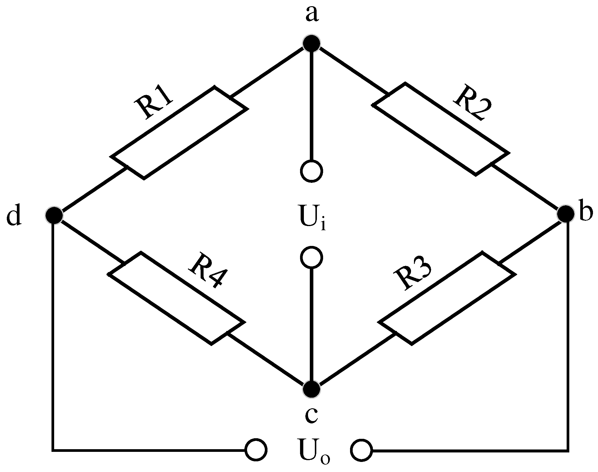
The drilling pressure measurement was based on the strain effect of resistive strain gauges using a Wheatstone bridge for the measurement process. As the resistive strain gauge was subjected to the stress imposed by the drilling pressure, its resistance changed. Therefore, it is essential to use a Wheatstone bridge to convert this change in resistance into a readable electrical signal, thereby achieving an accurate measurement of the drilling pressure.
Figure 1 illustrates the principles of the Wheatstone bridge. Owing to the harsh high-temperature conditions downhole, the resistive strain gauge exhibited nonlinear errors influenced by temperature. Temperature compensation is an indispensable step for ensuring the accuracy of drilling pressure measurements [
10,
11].
4. Principle of C-I-WOA-BP Neural Network
4.1. BP Neural Network
Owing to the nonlinear influence of temperature on resistive strain gauges, utilizing a BP neural network allows for a more precise modeling of this nonlinear relationship, thereby achieving effective compensation [
12].
Figure 2 shows the BP neural network architecture designed for temperature compensation, which comprises of input, hidden, and output layers. The input layer of the neural network incorporates the temperature Ut and output voltage Up from the drilling pressure measurement bridge. The desired output represents the actual force FN exerted by the drilling pressure, whereas the network output is the predicted drilling pressure,
. The hidden layer contains h neurons, the number of which is determined using the specific empirical formula
, where
m is the number of nodes in the input layer,
n is the number of nodes in the output layer, and a is an integer ranging from 1 to 10 [
13].
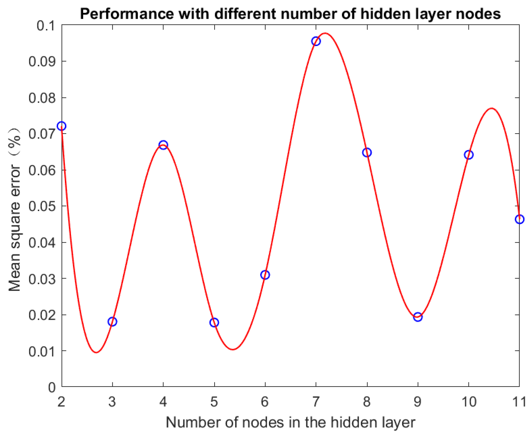
As shown in
Figure 3, the network achieved its minimum mean squared error when the number of neurons in the hidden layer was 5. Therefore, the 2-5-1 structure of the BP neural network is selected as the optimal configuration.
represents the weight from the
i-th neuron in the input layer to the
j-th neuron in the hidden layer, and
denotes the weight from the
j-th neuron in the hidden layer to the
k-th neuron in the output layer.
4.2. BP Neural Network Based on Whale Optimization Algorithm
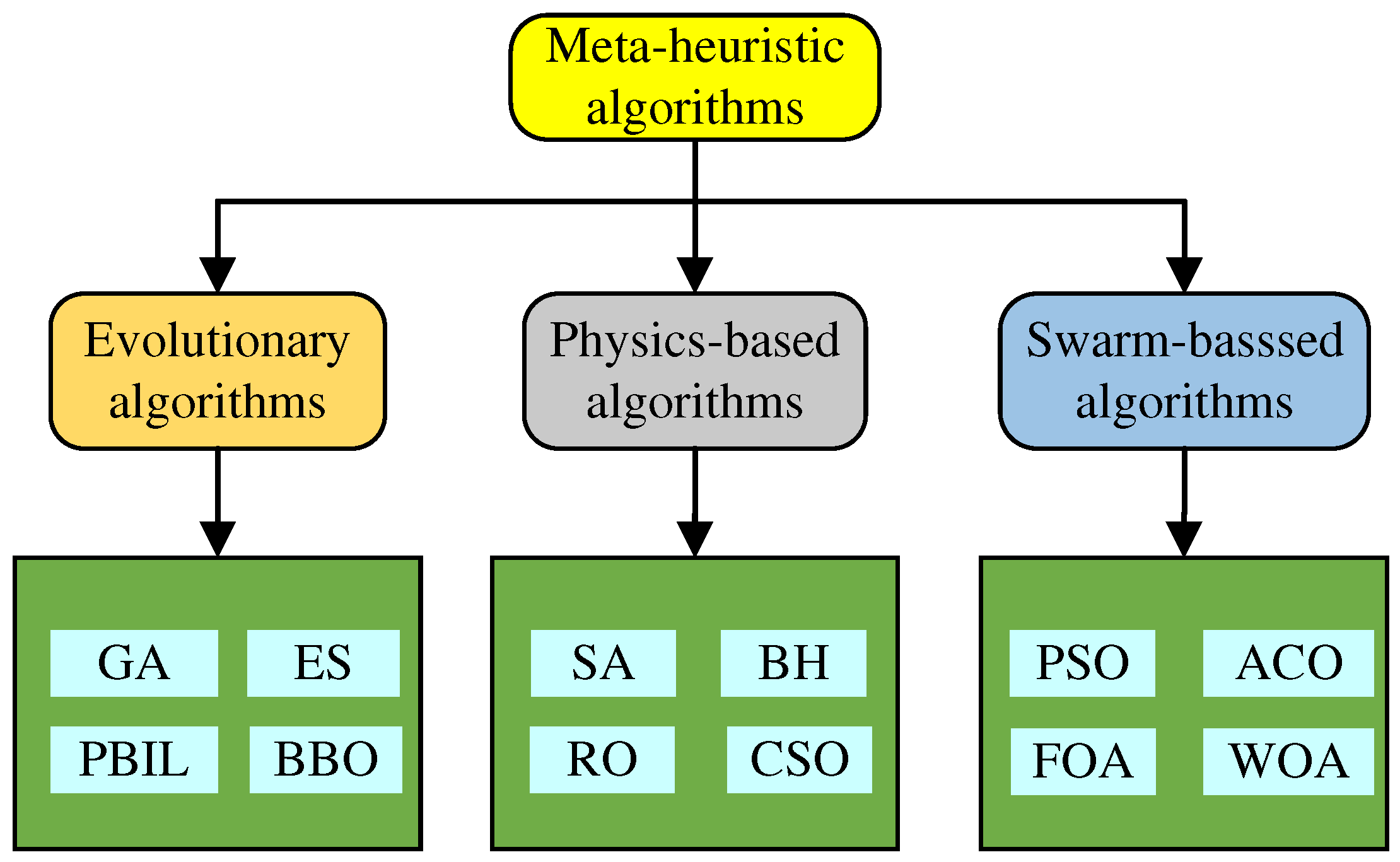
The WOA is a novel meta-heuristic optimization strategy inspired by the predatory behavior of humpback whales. Owing to their intuitive nature, ease of implementation, and the ability of meta-heuristic algorithms to operate without gradient information and avoid becoming trapped in local optima, they are gradually gaining widespread attention in engineering applications. Meta-heuristic algorithms can be broadly categorized into three main types [
14], as illustrated in
Figure 4. Meta-heuristic algorithms can be broadly categorized into three main types, as shown in
Figure 4. The first category includes intelligent optimization algorithms based on evolutionary principles, such as evolutionary strategies (ESs) and genetic algorithms (GAs). Next are intelligent optimization strategies grounded in the principles of physics, such as simulated annealing (SA) and black hole algorithm (BH). Lastly, there are intelligent optimization methods centered on swarm behaviors, including particle swarm optimization (PSO) and ant colony optimization (ACO), among others [
15].
The WOA is an intelligent optimization strategy based on swarm behavior. Its primary inspiration was drawn from the unique hunting techniques of humpback whales, such as encircling prey, bubble-net attacks (referred to as the exploitation phase), and searching for prey (also known as the exploration phase) [
16,
17]. By simulating these behaviors, we constructed a mathematical model of the WOA. The specific details of this model are as follows.
4.2.1. Encircling Prey
Encircling prey is based on a mathematical model constructed from the ability of humpback whales to identify and encircle gathered prey. This behavior can be described using the following mathematical expressions:
where
t is the number of iterations,
is the distance vector between an individual whale and the global optimum solution,
is the position vector of the whale with the best fit in the current iteration, and
is the position vector of the whale during the current iteration. The coefficient vectors
are used to adjust the search direction and step size.
The coefficient vectors
and
are expressed as:
In the equation,
is a random vector in the [0, 1] range,
is another random vector within the [0, 1] range, and
is an adjustment coefficient that linearly decreases from 2 to 0 during the iteration process. The magnitude of
was determined using:
where
t is the current iteration number, and
is the maximum number of iterations.
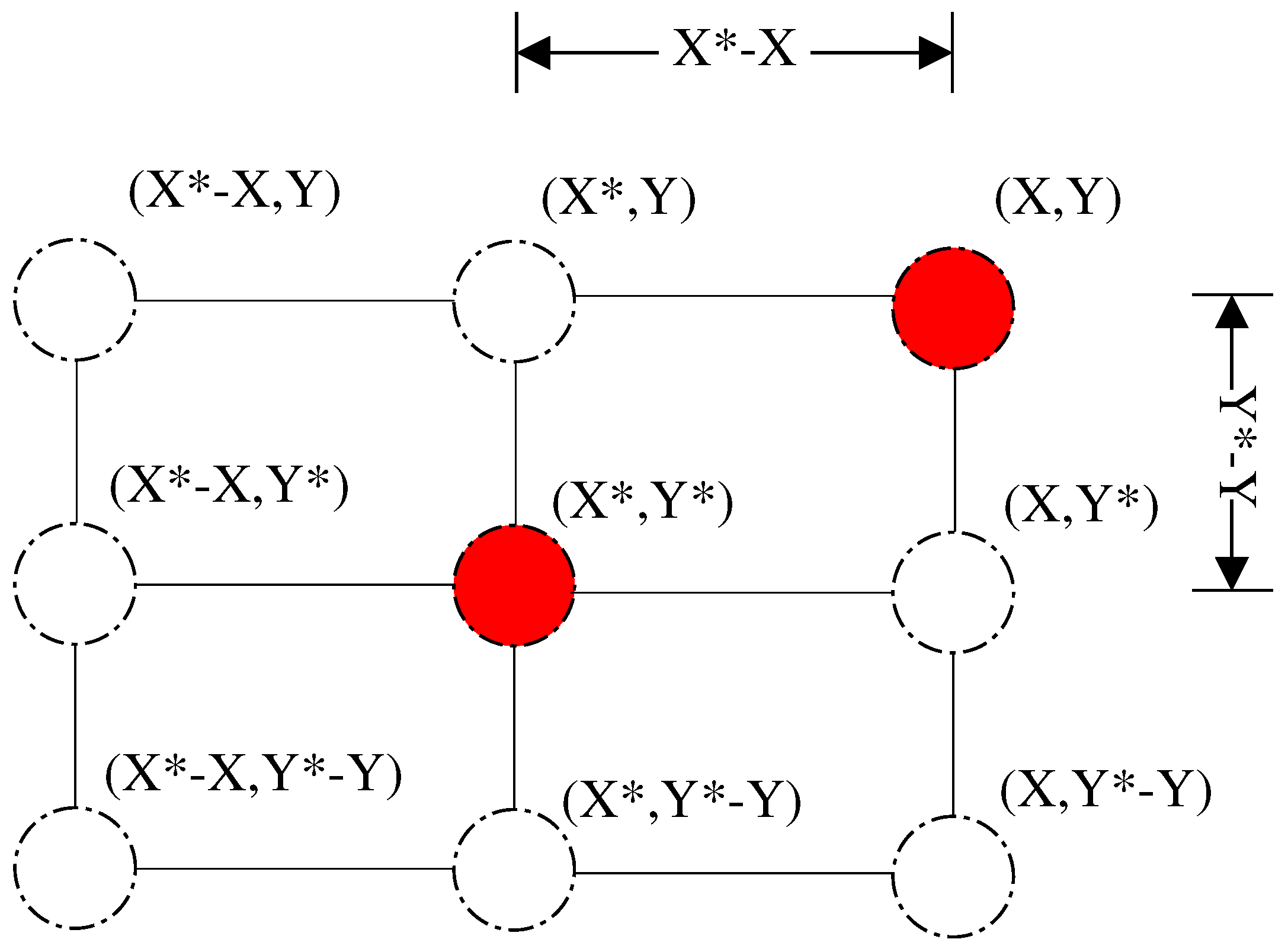
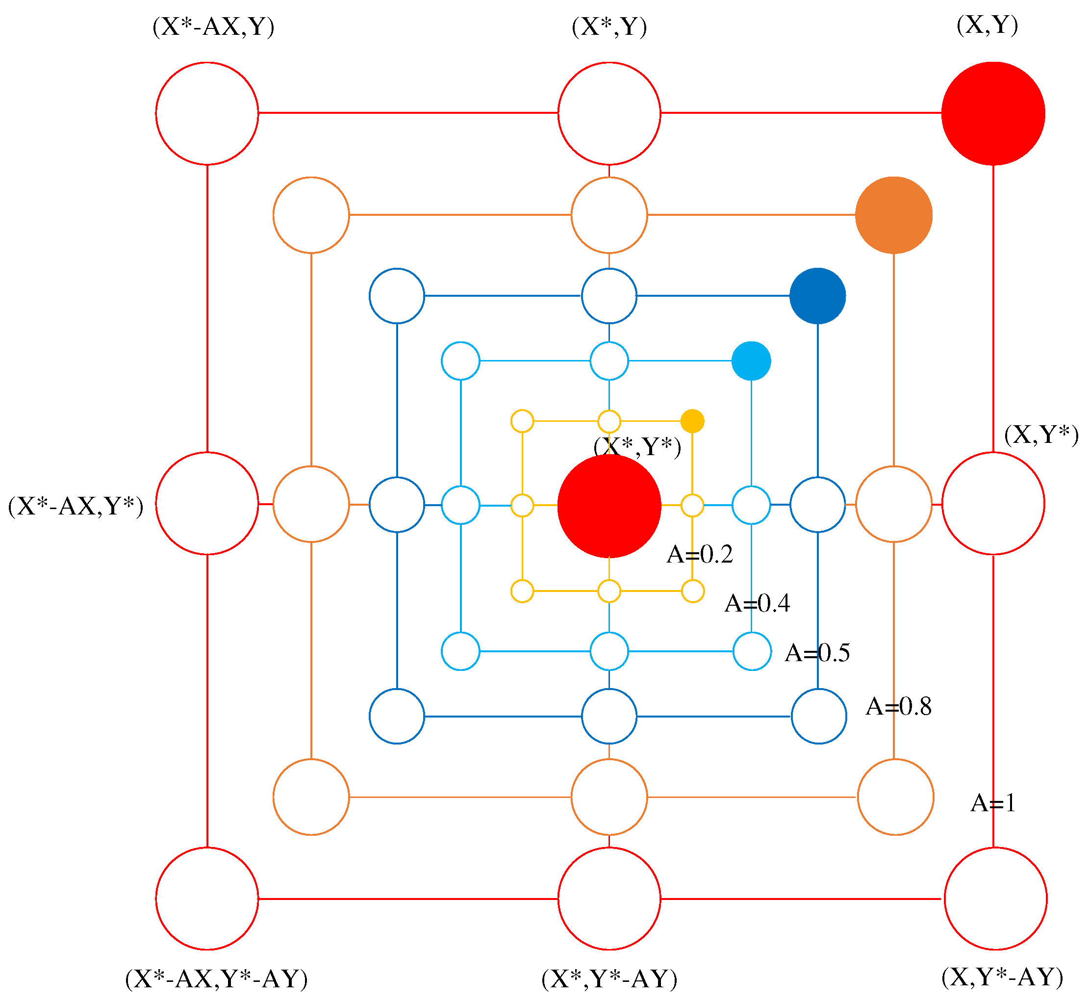
Figure 5 illustrates the underlying mechanism of prey encircling in a two-dimensional space. The position
of the whale in the current iteration is adjusted based on the optimal position
of the iteration. This adjustment was achieved by modulating the values of
and
using the alteration vectors
and
, respectively. Consequently, in the next iteration cycle, the whale can lie between the pivotal coordinates, as shown in
Figure 5. At every iteration, the whale updates its position to approach the current optimal position, mimicking the behavior of encircling the prey. The same principle applies to the higher-dimensional scenarios. For instance, in an n-dimensional space, the whale moves around the current best position within the n-dimensional space. In practical applications, n represents the number of variables in the solution to a problem.
4.2.2. Bubble-net Attacking Method
When a humpback whale preys on its target, it employs encircling contractions and spiral updating to approach the prey. Mathematical models were designed for both the shrinking encircling mechanism and the spiral-updating position strategy to simulate the predatory behavior of the humpback whale.
One shrinking encircling mechanism: This behavior is achieved by gradually reducing the value of parameter
in Eq.
3 during the iteration process, where the value of
is set within the interval
and linearly decreases according to Eq.
5 throughout the iteration process. When the value of parameter
is within the range
, the position of the whale in the next iteration can be chosen at any point between the current whale position and the optimal position. As shown in
Figure 6, in a two-dimensional space, when the value of parameter
is in the interval
, the possible position of the whale will be within the area formed by points
and
.
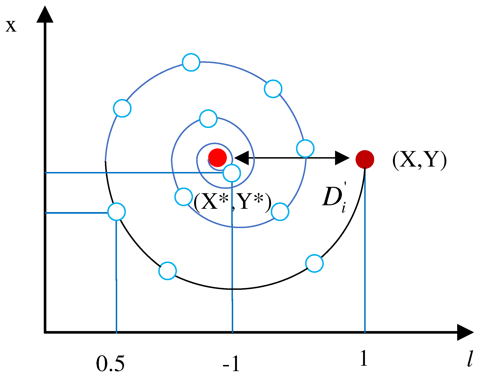
Two spiral updating position: As shown in
Figure 7, this strategy first determines the distance between the whale at coordinate point
and the current optimal position
. Subsequently, a spiral equation was established between
and
to simulate humpback whale spiral-hunting behavior. The spiral equation is given by
where
represents the distance from the coordinates of the
i-th whale to the optimal position, b is a constant used to define the logarithmic spiral contour, and
l is a parameter randomly selected from the interval
.
We assumed in the mathematical model that the probability of these two behaviors occurring was
to accurately simulate the humpback whale hunting process along a spiral path and the gradually narrowing circular swimming pattern. This was used to optimize the position of the whale during the iteration process. The mathematical model is as follows:
where
p is a random number in the interval
.
4.2.3. Search for Prey
In addition to the bubble-net attack method, whales engage in random searches for prey. This behavior is achieved based on the variation in the vector
when
is used. Compared to the bubble-net attack strategy, during the random search phase, the whale’s position
is updated based on the position of the randomly selected whale
. At this juncture, the position update does not gravitate toward the randomly selected whale but rather moves away from it. The underlying rationale for this strategy is to expand the search scope and achieve broader exploration, thereby preventing premature convergence to the local optima. Consequently, the position of the whale deviates from that of the reference whale during
. The mathematical model is expressed as:
where
is the vector distance between the current whale position and the position of the randomly selected whale, and
is the position vector of a whale randomly chosen from the current population.
The WOA is a swarm-based meta-heuristic search strategy. It starts with a set of randomly generated solutions, and as iterations progress, each whale individual updates its position based on the optimal individual position in the current iteration or based on the position of a randomly chosen whale. In addition, the value of the parameter
is gradually decreases linearly from2 to 0 to provide bubble-net attacking method and searching for prey, respectively. The whale positions are randomly selected to update the positions of the remaining whales in each iteration when condition
is met and the optimal position is chosen to update the positions of the remaining whales in each iteration when condition
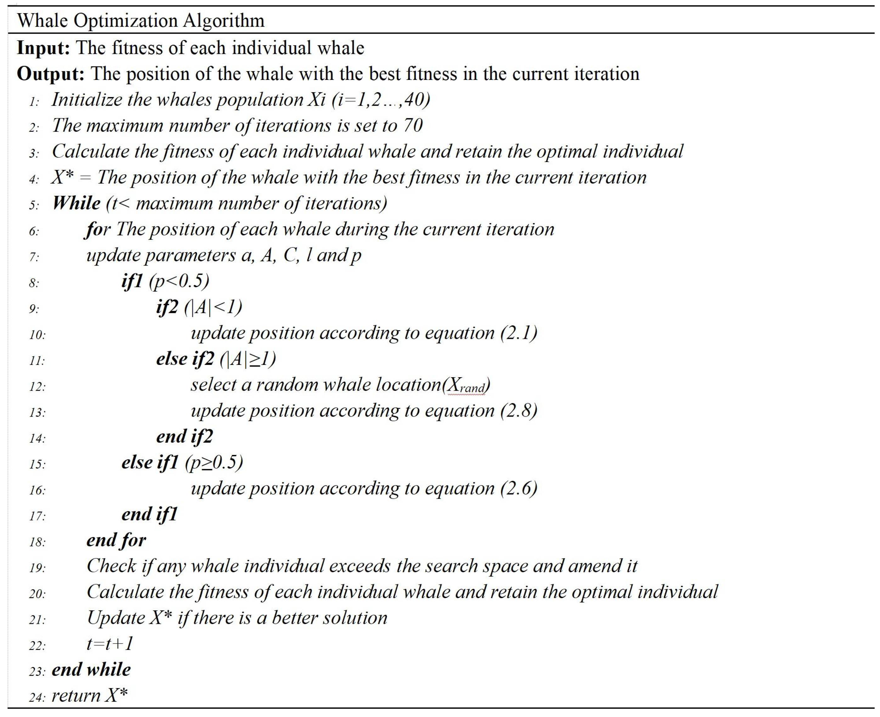
is met. Additionally, based on the random probability value p, the WOA can opt for either the shrinking encircle strategy or the spiral update strategy during position updates. Ultimately, the WOA algorithm concludes once specific termination criteria are met. The pseudo code of the WOA algorithm is presented in
Figure 8.
4.3. Whale Optimization Algorithm Improvement
The traditional WOA is advantageous in terms of simplicity, few control parameters, the ability to avoid local optima, and has been widely applied in numerous domains. However, the WOA has certain limitations in terms of the convergence speed and precision. To address this issue, an adaptive WOA based on chaos mapping, referred to as CIWOABP, has been proposed.
4.3.1. Chaotic Mapping Whale Optimization Algorithm
Chaos mapping generates chaotic sequences through the repeated application of iterative functions. It exhibits nonlinearity, high sensitivity to initial values, excellent ergodicity, and unpredictability [
18]. This mapping is frequently used for population initialization to enhance the algorithmic diversity and randomness [
19,
20]. Based on a comparison of 16 chaotic optimization algorithms in [
21], the maximum Lyapunov exponent of cubic mapping outperforms those of sine mapping, circle mapping, Liebovitch mapping, intermittency mapping, singer mapping, and Kent mapping. It is comparable to the exponents of logistic, sinusoidal, tent, Gaussian, and Bernoulli mapping but lower than the exponents of Chebyshev, ICMIC, and piecewise mapping [
22]. However, a holistic comparison revealed that the chaotic sequences generated by both Chebyshev and ICMIC mapping fell within the (-1,1) range. The formula complexity for piecewise mapping is high, and tent, Gaussian, and Bernoulli mapping use piecewise functions. Both sinusoidal and tent mappings tended to produce repetitive chaotic sequences. Therefore, considering all these factors, this study opted for cubic mapping to optimize the traditional whale algorithm. The formula is as follows:
where
, and
are control parameters.
4.3.2. Whale Optimization Algorithm for Combining Multiple Strategies
In the WOA, ensuring a balance between searching for prey and the bubble-net attack method is a key factor influencing the algorithm’s performance and accuracy (i.e., the dynamic switching between the search processes of eq.
7 and eq.
9). By appropriately adjusting the switching parameters and search methods, the algorithm’s flexibility and search efficiency can be enhanced [
23]. The inertial weight, which acts as a balancing parameter, has been widely applied in various metaheuristic optimization algorithms [
24,
25]. To achieve a better balance between the preying and searching phases and enhance the algorithm’s flexibility and search efficiency, we adjusted the value of the adaptive weight as follows:
where
is the adjustment coefficient,
is the current iteration number, and
is the maximum number of iterations. The adaptive weight gradually decreases as the number of iterations increases. In the first half of the search for prey and the bubble-net attack phase, a larger inertia weight can enhance the global search performance, prompting a deeper exploration of potential global optima by the algorithm, thus helping the algorithm avoid getting stuck in local optima. In the second half of the search, as the inertia weight decreases, the local search capability is strengthened, allowing the algorithm to find the optimum solution faster within a smaller search space, thereby accelerating the algorithm’s convergence process. After incorporating the dynamic adaptive weight value adjustment, the improved strategies for encircling prey, bubble-net attacks, and searching for prey can be represented by the following equations:
5. Temperature Error Compensation
5.1. Calibration Data for Drilling Pressure Parameters
A Honeywell ASDX100D44R pressure sensor and PT100-RTD temperature transmitter were used in the laboratory. In this experimental configuration, the temperature measurement range was set between 0°C and 78°C, with measurement points set at 6°C intervals, yielding a total of 14 measurement points. For pressure, the measurement range was from 40 kPa to 80 kPa, with measurement points arranged at 5 kPa intervals, resulting in a total of nine measurement points.
Table 1 lists the calibration data for the pressure sensor, where p is the applied pressure in the experiment, Up is the output voltage signal, and Ut is the actual measured temperature.
5.2. Temperature compensation
In this study, we utilized Up and Ut as input parameters for the neural network, and the pressure p was set as the output value of the neural network. To ensure the efficiency and accuracy of network training, we selected pressure sensor calibration data at 0 °C, 6 °C, 18 °C, 24 °C, 36 °C, 42 °C, 54 °C, 60 °C, 72 °C, and 78 °C as the training dataset, while the data at 12 °C, 30 °C, 48 °C, and 66 °C were chosen as the test dataset. Furthermore, all data were normalized to ensure that the values fell between 0 and 1 and achieve optimal network performance. The constructed BP neural network structure was 2-5-1, with two input layers, five hidden layers, and one output layer. In the CIWOA configuration, we set an initial population size of 40 with a maximum iteration count of 70. The control parameter in the cubic mapping function was set to 1, and the adjustment coefficient mm in the adaptive weight adjustment function was set to 1. Because the results of the neural network training may vary with each iteration, we opted for multiple training sessions and ultimately utilized the compensated data from the test samples, as shown in
Table 2.
5.3. Analysis of Results
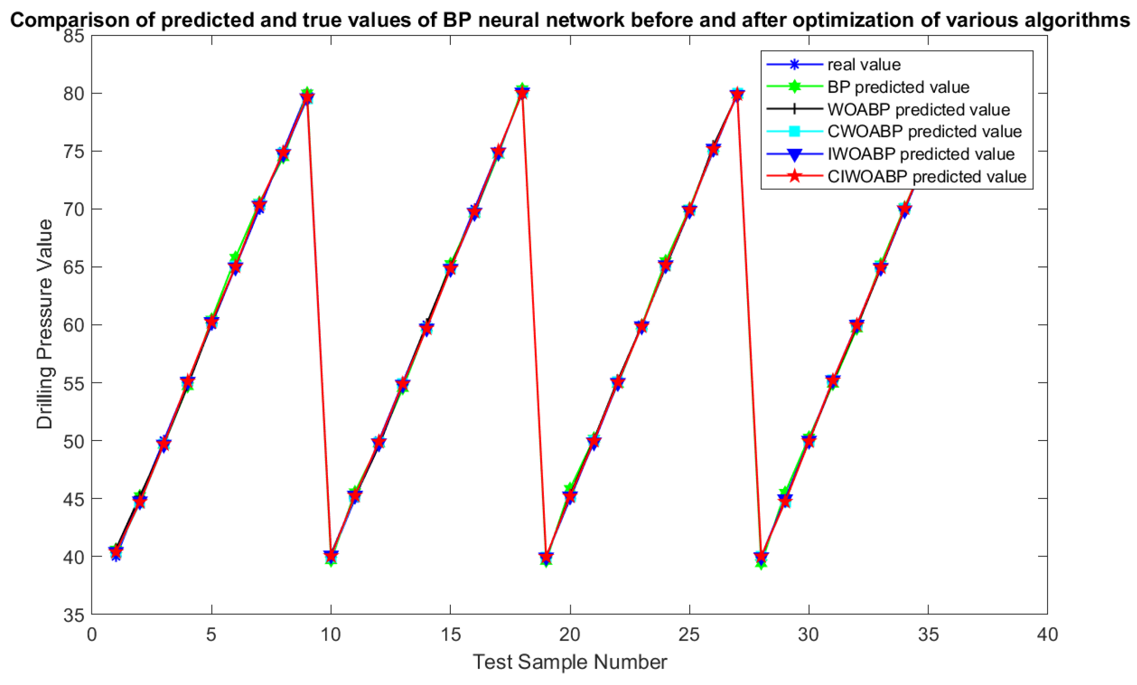
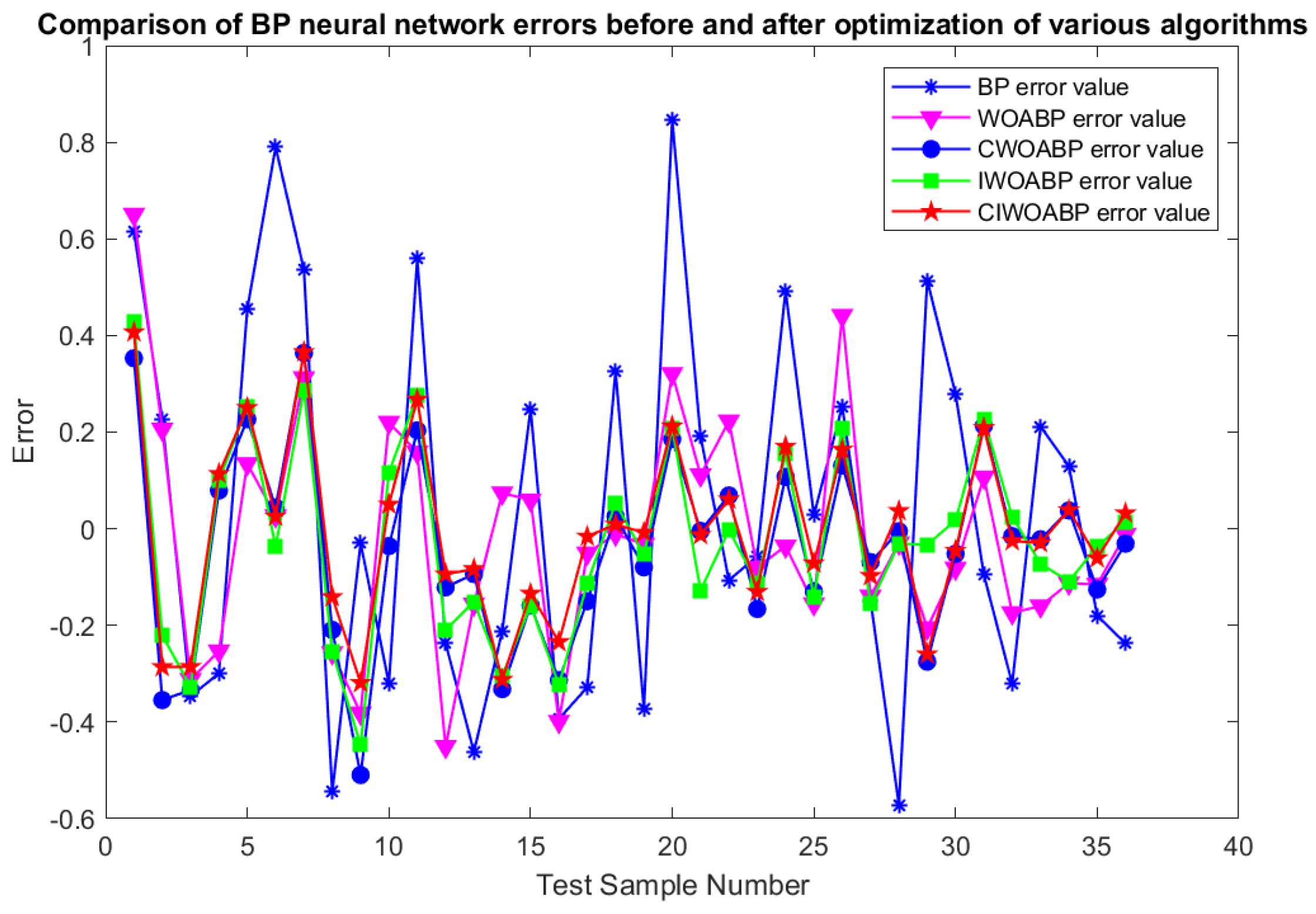
To validate the performance of the proposed algorithm thoroughly, we employed five distinct neural network architectures: BP, WOABP, CWOABP, IWOABP, and CIWOABP. These networks were trained using test samples. A comparison between the values predicted by the BP neural network before and after optimization with each algorithm and the actual values is illustrated in
Figure 9. An error comparison of the BP neural network before and after optimization with each algorithm is shown in
Figure 10.
In
Figure 9 and
Figure 10, we can observe that, compared to the other optimization methods, the error of the temperature compensation using the CIWOABP neural network is noticeably smaller, with the error range consistently within 0.4. We listed the error comparison results for the different temperature compensation models in
Table 3. to further evaluate the performance of each algorithm.
Based on
Table 3, the temperature compensation model using CIWOABP outperformed the other models across various evaluation metrics, including the sensitivity temperature coefficients, mean absolute error, mean square error, and mean absolute percentage error.
6. Conclusions
In this study, a sophisticated temperature compensation technique that leverages a CIWOABP neural network was introduced. This approach synthesizes the unmatched precision of the BP neural network with the streamlined control parameters of the WOA due to its advantages in circumventing local optima. It also capitalizes on the swift convergence attributes of the CWOA and draws on the expansive global search and meticulous local refinement capacities of the IWOA algorithm. It boasts advantages such as exceptional accuracy, innate resilience against being ensnared in local optima, rapid convergence velocities, and formidable capabilities in global searching and local refinement. This effectively addresses the conventional limitations of the BP neural network, such as the environment in local optimal solutions and lethargic convergence. The refined pressure sensor measurement system achieved a sensitivity temperature coefficient of , and the average absolute percentage deviation stood at a mere , satisfying the pragmatic operational benchmarks.
Author Contributions
Fei Wang was responsible for the overall structure of the article and the design of the algorithm. Xing Zhang and GuoWang Gao took charge of the experimental section in the paper and the writing of the article and Xintong Li assisted with the experiments and provided linguistic modifications.
Funding
The Project supported by the Shaanxi Province Key R&D Program Project (No. 2022GY-435).
References
- Bai, J.; Zhang, B.; Zhang, C.P. Status quo and development proposal of ultra-deep and ultra-small borehole directional drilling technology. Drilling Process 2018, 41, 5–8+143. [Google Scholar]
- Zhu, Z.F.; Zhang, H.N. Research on nonlinear calibration and temperature compensation method of pressure transmitter. Electronic Measurement Technology 2021, 44, 71. [Google Scholar]
- Wu, C.H.; Jiang, R.W. Temperature compensation method for pressure sensor based on PSO-LM-BP neural network. Instrumentation Technology and Sensors 2018, 129–133. [Google Scholar]
- Liu, H.; Li, H.J. Research on temperature compensation method of pressure sensor based on BP neural network. Journal of Sensing Technology 2020, 33, 688–692+732. [Google Scholar]
- Wang B B, L.H.J. Temperature compensation of silicon piezoresistive pressure sensor based on cubic spline interpolation. Journal of Sensing Technology 2015, 28, 1003–1007. [Google Scholar]
- He, R.; Xiao, X.; Kang, Y.; Zhao, H.; Shao, W. Heterogeneous Pointer Network for Travelling Officer Problem. In Proceedings of the 2022 International Joint Conference on Neural Networks (IJCNN); IEEE, 2022; pp. 1–8. [Google Scholar]
- He, X.; Trigila, C.; Ariño-Estrada, G.; Roncali, E. Potential of depth-of-interaction-based detection time correction in Cherenkov emitter crystals for TOF-PET. IEEE Transactions on Radiation and Plasma Medical Sciences 2022, 7, 233–240. [Google Scholar] [CrossRef]
- Ding H, Li J, S.H.L.e.a. Dual-path temperature compensation technique for fiber optic transformer based on the least squares method. Electronic Measurement Technology 2016, 39, 190–195.
- Lv M C, L Q Q, S.X.e.a. Design of infrared temperature sensor based on GA-BP neural network temperature compensation. Instrumentation Technology and Sensors 2019, 03, 19–22.
- Ma, H.G.; Zeng, G.H.; Huang, B. Research on temperature compensation of pressure transmitter based on WOA-BP. Instrumentation Technology and Sensors 2020, 33–36. [Google Scholar]
- Zhou, Z.W.; Deng, T.Y.; Shi, L.; et al. Temperature compensation and field calibration method for piezoresistive pressure sensors. Sensors and Microsystems 2022, 41, 145–148. [Google Scholar]
- Liu, H. Optimal selection of control parameters for automatic machining based on BP neural network. Energy Reports 2022, 8, 7016–7024. [Google Scholar] [CrossRef]
- Zhang, R.; Duan, Y.; Zhao, Y.; et al. Temperature Compensation of Elasto-Magneto-Electric (EME) Sensors in Cable Force Monitoring Using BP Neural Network. Sensors 2018, 18, 2176. [Google Scholar] [CrossRef]
- Shao, W.; Jin, Z.; Wang, S.; Kang, Y.; Xiao, X.; Menouar, H.; Zhang, Z.; Zhang, J.; Salim, F. Long-term spatio-temporal forecasting via dynamic multiple-graph attention. arXiv 2022, arXiv:2204.11008. [Google Scholar]
- Mirjalili, S.; Lewis, A. The whale optimization algorithm. Advances in Engineering Software 2016, 95, 51–67. [Google Scholar] [CrossRef]
- Xu, D.G.; Wang, Z.Q.; Guo, Y.X.; et al. A review of research on whale optimization algorithms. Computer Application Research 2023, 40, 328–336. [Google Scholar]
- Sun, Y.; Wang, X.; Chen, Y.; et al. A modified whale optimization algorithm for large-scale global optimization problems. Expert Systems with Applications 2018, 114, 563–577. [Google Scholar] [CrossRef]
- Kang, Y.; Rahaman, M.S.; Ren, Y.; Sanderson, M.; White, R.W.; Salim, F.D. App usage on-the-move: Context-and commute-aware next app prediction. Pervasive and Mobile Computing 2022, 87, 101704. [Google Scholar] [CrossRef]
- Li, M.; Xu, G.; Lai, Q.; et al. A chaotic strategy-based quadratic Opposition-Based Learning adaptive variable-speed whale optimization algorithm. Mathematics and Computers in Simulation (MATCOM) 2022, 193. [Google Scholar] [CrossRef]
- Wu, G.; Li, Y. Non-maximum suppression for object detection based on the chaotic whale optimization algorithm. Journal of Visual Communication and Image Representation 2023, 74. [Google Scholar] [CrossRef]
- Feng, J.H.; Zhang, J.; Zhu, X.S.; et al. A novel chaos optimization algorithm. Multimedia Tools & Applications 2016. [Google Scholar]
- Zhang, M.j.; Zhang, H.; Chen, X.; et al. Gray wolf optimization algorithm based on Cubic mapping and applications. Computer Engineering and Science 2021, 43, 2035–2042. [Google Scholar]
- Deng, H.; Liu, L.; Fang, J.; et al. A novel improved whale optimization algorithm for optimization problems with multi-strategy and hybrid algorithm. Mathematics and Computers in Simulation (MATCOM) 2023, 205. [Google Scholar] [CrossRef]
- Rauf, H.T.; Malik, S.; Shoaib, U.; et al. Adaptive inertia weight Bat algorithm with Sugeno-Function fuzzy search. Applied Soft Computing 2020, 90, 106–159. [Google Scholar] [CrossRef]
- Li, X.N.; Wu, H.; Yang, Q.; et al. A multistrategy hybrid adaptive whale optimization algorithm. Journal of Computational Design and Engineering 2022, 9, 1952–1973. [Google Scholar] [CrossRef]
|
Disclaimer/Publisher’s Note: The statements, opinions and data contained in all publications are solely those of the individual author(s) and contributor(s) and not of MDPI and/or the editor(s). MDPI and/or the editor(s) disclaim responsibility for any injury to people or property resulting from any ideas, methods, instructions or products referred to in the content. |
© 2023 by the authors. Licensee MDPI, Basel, Switzerland. This article is an open access article distributed under the terms and conditions of the Creative Commons Attribution (CC BY) license (http://creativecommons.org/licenses/by/4.0/).
