Preprint
Article
Assistive Learning Intelligence Navigator (ALIN) Dataset: Predicting Test Results from Learning Data
Altmetrics
Downloads
85
Views
30
Comments
0
This version is not peer-reviewed
Submitted:
28 October 2023
Posted:
31 October 2023
You are already at the latest version
Alerts
Abstract
Data mining techniques have garnered significant attention within the realm of education. However, the procurement of ample student data poses a formidable challenge. In response to this challenge, we present a student dataset characterized by its size and distinctive attributes. This dataset encompasses various task-related topics interconnected through a learning pathway, thereby enabling researchers to delve into the data from novel perspectives. Moreover, it encompasses extensive longitudinal student behavioral data, a rarity that adds substantial value. Spanning the years from 2010 to 2021, our dataset comprises a cohort of 7,933 students, 64,344 test scores, and 183,390 behavior records, solidifying its status as a valuable resource for educational research. In our experiments, we achieved successful predictions of students' test outcomes based on behavioral learning data. The strengths of our dataset render it apt for analyzing the nexus between student conduct and academic performance, crafting personalized learning recommendations, and pursuing various other research pursuits.
Keywords:
Subject: Computer Science and Mathematics - Computer Science
1. Introduction
Educational data mining (EDM) involves the application of data mining techniques within the field of education. Various tasks, including performance prediction and personalized recommendation, have been proposed and explored in this area. The accuracy and efficacy of these endeavors, however, heavily rely on the availability of student data for analysis. Despite the emergence of datasets like ASSISTments 2009-20101, their pertinence may have waned over the last decade. Consequently, there is an imperative need for up-to-date learning behavior data.
Our examination of EDM research underscores that the amount of data employed in recent studies falls short. For instance, Kaur et al. (2015) scrutinized a dataset comprising only 152 high school students to forecast academic performance and discern sluggish learners. Similarly, Amrieh et al. (2016) harnessed educational data from a mere 500 students to train an ensemble classifier for academic performance prediction. You (2016) amassed data from 530 college students enrolled in an online course, identifying numerous behavioral cues for projecting final course scores.
Table 1 organizes and juxtaposes the datasets utilized in the aforementioned studies. The tabulated data reveals that the student count in these investigations remains below 600. Regrettably, all the datasets employed in the research are proprietary, posing challenges to their reuse for comparative purposes. The dearth of student data has emerged as a pivotal constraint within EDM (Zhao et al., 2021). Furthermore, the bulk of these datasets are derived from high school or university students, leaving an insufficiency in pupils' learning data. As a remedy, we are disseminating an extensive dataset of primary school students' learning behaviors, sourced from an adaptive learning website (www.alin.ai).
As an educational technology company, ALIN (Assistive Learning Intelligence Navigator) successfully operates an online adaptive learning platform that assists students in learning mathematical knowledge. Learning math requires a lot of practice and timed exercises that test for both accuracy plus speed. Based on our interviews and anecdotes, students stress over these exercises and even cry when given tasks that are too difficult for their current capability. Moreover, we also will redefine student success away from solely using test scores to the whole child development approach. This goal requires a live research platform which we are calling ALIN.ai that will provide free math lessons with attention training interspersed throughout the lessons to deal with stress, not just learn math. It will be used to show objective measures of student success even without having to teach to the test or score-based metrics that drive prevailing approaches in today’s Education field. Based on the taxonomy presented in Romero and Ventura's report (2010), ALIN can be categorized as an intelligent tutoring system (ITS). Unlike conventional systems that merely present content on the web, ITS represents an innovative approach to learning, aiming to customize instruction to the unique needs of individual students. Typically, an ITS comprises four key components: the domain model, tutoring model, student model, and interface (Pai et al., 2021). Among these, the domain model holds particular significance as it encompasses a wealth of domain-specific expertise, including domain knowledge and adaptive rules (Alkhatlan & Kalita, 2018).
Similarly, on the ALIN website, experts have meticulously constructed a knowledge graph by breaking down the math curriculum into finely-grained topics. For example, addition might be split into FastAdd, LongAdd0, LongAdd, DecAdd, IntAdd, and other subcategories. Worksheets are timed-drill-problem sets from a given topic that trains both accuracy and speed. Assessments or tests are adaptive binary searches to find the frontier of knowledge of a student from basic skills or core skills depending on the grade level. Given both accuracy and speed requirements, reaching mastery of a topic in the learning platform correlates highly with students' knowledge. While students are learning on ALIN, the data of the learning behavior and results are recorded in the database. The historical learning data is related to some prescribed learning sequences covering K-12 up and Geometry proofs.
EdTech (educational technology) shows great promise but also grapples with extended deployment timelines among students. One reason is the multitude of education stakeholders, yet the student's learning should remain paramount. Still, test scores typically serve as the primary metric for assessing the impact of the learning environment, including most EdTech solutions. This renders student data exceedingly valuable, especially in the AI/ML-driven era, leading many organizations to hesitate in sharing their data. Consequently, most studies are reluctant to make their datasets public. Our aim is to disrupt this counterproductive incentive cycle by offering two public datasets for the entire education community, enhancing the quality of math education for students.
To solve the lack of student data as described above, we are pleased to publish two student datasets publicly in this study. We hope the datasets will help the researchers to perform wider and deeper studies relevant to EDM. Utilizing the datasets, a wild range of research can be executed, such as behavior analysis, performance prediction, learning recommendation, and so on. To present the applications of the datasets, we separately conduct two experiments to predict students’ performance. To enable reproducibility, we share datasets and baseline models on GitHub2 and IEEE Dataport3.
2. Literature Review
In this work, one of our objectives is to make a prediction of students’ test results using their historical learning data. It is similar to the task of performance prediction mentioned by Romero and Ventura (2010). We surveyed some studies published in recent ten years, and some similar and helpful works are described as follows.
Xu, Yuan, and Liu (2020) undertook a research endeavor that involved the amalgamation of online and offline learning data to explore the predictability of student performance. Their study demonstrated that online learning data could indeed be harnessed to predict student achievements, with a focus on assignment-related attributes as potential predictors. This approach allowed for the analysis and projection of students' learning progress based on general online learning behaviors and, in particular, behaviors related to assignments. Hamsa et al. (2016) aimed to discern students' performance in individual subjects. Their approach encompassed the construction of a prediction model utilizing a decision tree in conjunction with a fuzzy genetic algorithm. Features for the model were extracted from two exams and academic records spanning specific time periods. Similarly, Saa (2016) focused on educational data analysis, with a particular emphasis on students' performance. The study delved into a range of factors including personal and social variables, employing various classifiers to forecast performance. Shahiri and Husain (2015) conducted a comprehensive literature review centered around forecasting student performance. The investigation examined how prediction algorithms could effectively identify pivotal attributes from student data. Their findings underscored the recurring use of attributes like Cumulative Grade Point Average (CGPA) and internal assessments as integral predictors. Importantly, these findings align with our perspective, given that our dataset originates from primary school students, with CGPA akin to the average accuracy of problem-solving and our system's tests resembling internal assessments. Ha et al. (2020) harnessed diverse machine learning techniques to predict students' final Grade Point Average. Their research uncovered a correlation between student performance and various factors including academic progress, personal traits, and behaviors associated with learning activities.
Since 2015, deep models have catalyzed the emergence of various iterations of deep knowledge tracing (DKT). In the work of Piech et al. (2015), Recurrent Neural Networks (RNNs) were employed, utilizing all preceding student interactions as input to make predictions. Su et al. (2018) enhanced this approach by incorporating an attention mechanism into the RNN, enabling the computation of a weighted aggregation of prior knowledge states. Abdelrahman and Wang (2019) proposed a hop-LSTM architecture designed to capture long-term dependencies in exercise sequences, while simultaneously delving into the specific concepts within a student's knowledge state. Vie and Kashima (2019) introduced factorization tracing machines (KTM) to monitor students' learning progress, taking into account auxiliary information such as multiple skills for each student, leading to improved predictive performance. More recently, Minn et al. (2022) introduced a concise and efficient model with interpretable factors like skill mastery, ability profiles, and problem difficulty to model student performance. Impressively, their results surpassed those of several deep learning-based models, despite having a significantly smaller model size.
The above studies revealed some important types of features and effective algorithms for performance prediction. In the following parts, we will describe our datasets and explain the features extracted from the data.
3. Dataset
The data presented in this paper originates from ALIN and is closely interconnected with ALIN's learning scenarios. We are hereby making available two distinct types of datasets: “learning beyond test” and “learning with test”. Within the first dataset, information is gathered from 4,966 students, encompassing 223,470 statistical metrics derived exclusively from the learning progression. In comparison, the second dataset encompasses not only learning-related data (183,390 behavioral records) but also examination data (64,344 test scores) from a cohort of 5,195 students. Subsequent sections will provide an introduction to these datasets along with an elucidation of the significance behind each terminology.
3.1. Learning beyond Test
Students' learning process and results are recorded over time. We applied various statistical functions to the raw sequence of data records such as maximum, minimum, average, and we constructed 43 features in total. The features may reflect the characteristics of different students, such as the amount of exercise done and the response time during the exercise. The ground truth consists of averaged correctness and averaged time spent on testing problems. Due to page limitations, only a portion of the descriptors are listed in Table 2. The engaged time in the raw data means how much time a student has spent on learning. The number of works attempted in the raw data means the number of worksheets finished by a student, and a worksheet is where a student practices solving math problems. The problems completed reflect the amount of work a student has done. The mastered topics refer to those topics a student has passed with a certain correctness threshold. Related scenarios can be found on the website. The complete features can be found in our public repository.
3.2. Learning with Test
As previously mentioned, ALIN is utilized by both students and teachers. Students have the ability to follow their respective teachers, who can then assign tasks to them. Typically, students are required to undertake two assessments: one prior to learning and another after a period of learning, which serves to gauge their progress.
Each assessment comprises multiple sequences, with each sequence containing a set of topics. Within each topic, a series of problems is provided for students to solve. During the assessment process, various metrics are recorded for each student's performance on individual topics. These metrics include the total number of problems attempted, the percentage of correct answers, the time taken, and other relevant information. The evaluation mechanism employs rule-based criteria based on topic performance to assign scores to each sequence within the assessment. Consequently, the cumulative score of the entire assessment is calculated by summing up the scores of all sequences it comprises.
To construct the dataset, we specifically chose students who have completed exactly two assessments. Moreover, there is a prerequisite that the time interval between these two assessments exceeds one week, thereby allowing ample time for studying and practice. For eligible students, both their assessment data and learning data were collected. It's important to note that our data collection solely encompassed behavioral information recorded during the two assessments. Subsequently, we matched the assessment data with the corresponding learning data for each student. The order and structure of the collected data are visually depicted in Figure 1.
Using the compiled dataset, we have outlined a set of primary terms, which are presented in Table 3. Terms labeled with names prefixed by “test” are extracted from the initial test records, whereas those beginning with “beh” are derived from learning behavior records. It's important to note that while students are generally encouraged to engage in learning and practice activities during the two assessment periods on the platform, participation is not mandatory. Consequently, the dataset includes students with varying degrees of behavior records: some have complete records, others possess partial records, and a few have no behavior records at all. When a student undertakes exercises, the system captures behavior-related information, such as the count of correct/incorrect/skipped problems. The term "skipped problems" pertains to unanswered questions, which might occur due to the difficulty of the problem or time constraints. As previously discussed, a typical test encompasses a series of sequences, with each sequence containing multiple topics. Students are required to complete a worksheet of relevant problems when testing or practicing a particular topic. Within a test, each topic necessitates only one worksheet, but during practice sessions, students can work on numerous worksheets without constraints. Consequently, terms derived from test data are focused on the topic level, while terms extracted from behavior data pertain to the worksheet level. The initial and final data points denote a student's performance in the first and last test sequence, respectively. Notably, not every student possesses all terms, as some students exclusively complete the two required tests without engaging in learning or practice activities on the ALIN platform.
Building upon the original terms, we have generated additional features, as presented in Table 4. These features are drawn from both test and behavior data, either by topic or by sequence. Furthermore, the values of these features are normalized to a range between 0 and 1. It's worth mentioning that the normalization process operates at the sequence level due to variations in scale across different sequences. Prior to normalization, the dataset is segmented into distinct groups based on sequenceID, ensuring that records within each group belong to the same sequence. The normalization process is then applied independently to each group, facilitating accurate treatment of values with differing scales. Armed with these features, our experimental approach involves training various machine learning models to predict sequence points and the overall score in the final test.
4. Challenge
Within the realm of educational data mining, there exist significant challenges that are both crucial and intricate to address. These challenges can be categorized into two main types: social challenges and technological challenges (Ang et al., 2020). Social challenges encompass issues such as student performance analysis and privacy protection. Evaluating a student's performance and determining whether they should progress to more advanced content involves analyzing learning data. Simultaneously, it's essential to safeguard the privacy of student-related information. On the other hand, technological challenges encompass practical considerations like system deployment, data collection, and data preprocessing.
In a related context, Baker (2019) highlighted additional challenges for the future of educational data mining during the 9th International Conference on Learning Analytics and Knowledge. These challenges revolve around the attributes of forecasting models, including their transferability, effectiveness, interpretability, applicability, and generalizability. An ideal model should have the capacity to transition seamlessly between different learning systems, demonstrating that intervention groups outperform non-intervention groups. This model should also trace changes in knowledge and forecast future student performance across various learning scenarios.
The challenges faced in our current work mirror those previously mentioned. Since we are working with student data derived from an online learning platform, we lack direct control over student behavior. Consequently, meticulous data collection and preprocessing are necessary to ensure data quality. Moreover, given the diversity in student behaviors, it becomes imperative to develop a generalized model that accommodates the variations among students. Our ultimate goal involves training a model capable of predicting student performance while also providing insights into the model's decision-making process.
In our experimental phase, we employ two distinct models: a regression model and the GBRT (Gradient Boosted Regression Trees) model. The aim is twofold: firstly, to predict student performance utilizing the GBRT model, and secondly, to elucidate crucial determinants via the regression model. This dual approach facilitates both prediction and explanation, enhancing our understanding of student performance factors.
5. Methodology
5.1. Learning beyond Test
Regarding the “learning beyond test” dataset, our objective was to forecast the average correctness and average time spent by students based on their historical learning behavior. To gain a more insightful understanding of student attributes, delving into their individual profiles is crucial. Traditionally, student profiles encompass fundamental details like gender, location, age, grade level, and the like. However, by utilizing our suggested descriptors, we can extract significant labels from the dataset using expert insights, particularly those garnered from teachers' experience. For instance, consider the correlation depicted in Figure 2 between calculation speed and a diligent work ethic. These descriptors allow us to create labels that add depth to our analysis.
Another illustrative example is presented in Figure 3. Our observations reveal that certain students tend to solve math problems rapidly and with haste. This behavior could be indicative of a distinct cognitive trait. Notably, the solid box denotes outstanding students, while the dashed box represents those with untapped potential. These latter students exhibit a pattern of expending minimal time on tests while achieving moderate levels of correctness. It's reasonable to assume that their scores could substantially improve if they adopt a more patient and time-intensive approach. When these students already achieve relatively high test scores, their potential for further improvement becomes evident, provided they develop greater patience. As such, the identification of such students holds considerable significance for tailoring interventions focused on patience development.
Moreover, leveraging the 43 statistical descriptors, we employed the K-means algorithm to cluster a total of 4,966 students. The choice of K value was determined through consideration of the silhouette score for clustering results, as depicted in Figure 4 (a). The optimal silhouette score emerged with a K value of 3, leading to the formation of three distinct student clusters. Illustrated in Figure 4 (b), these clusters encompassed 2,823, 1,741, and 402 students respectively. Building on these cluster outcomes, we conducted a detailed analysis of descriptor distributions to enhance our ability to forecast test results.
The flowchart of prediction is shown in Figure 5. We select and compare four predictors, Light Gradient Boost Machine (LightGBM), Random Forest (RF), Deep Neural Network (DNN), and eXtreme Gradient Boosting (XGBoost). Concretely, LightGBM is a machine learning algorithm based on the decision tree. RF is an ensemble learning algorithm that integrates the results of multiple decision trees into one for prediction. DNN is a fully connected neural network with an input layer, an output layer, and several hidden layers, and it can be utilized for classification and regression. XGBoost is a boosting algorithm that uses a greedy algorithm to search leaf nodes. These predictors will be trained on the training set and applied to predict the targets on the testing set. Moreover, the results of XGBoost will be selected as the baseline and compared with the results of the other predictors.
5.2. Learning with Test
Additionally, one of the primary goals of this study is to predict students' test performance using their past test and learning data. To illustrate this, consider the “learning with test” dataset, wherein each student has undertaken similar tests on two occasions, and our prediction target is the performance of their final test.
The assessment of test performance relies on two key metrics: points and score. Points serve as an evaluation metric for a sequence based on the corresponding answer outcomes. The value of points is determined by the count of topics with a perfect 100% correct rate within the sequence. Furthermore, a test's score is the summation of sequence points belonging to it. Since the score can be derived from sequence points, the task of predicting test results involves training a model to forecast the point value for each sequence within a test.
Notably, we hypothesized that the last point may exhibit some level of correlation with the first point for the same sequence. Our calculation of the correlation between these two points yielded approximately 0.718, signifying a significant positive correlation. This suggests that using the first point as a feature in the predictive model could be beneficial. This finding aligns with the observations made in Shahiri and Husain’s report (2015).
In order to analyze the distinction between the first and last points, we computed the difference for each student's sequence by subtracting the first point from the last point. This difference could be positive, negative, or zero. Our rationale was that this difference might offer insights into the learning behavior shift between the two tests. However, as previously discussed, behavior records are available for only a subset of students, leaving others without such records. Consequently, we divided the dataset into two subsets: the “With-behavior” set, comprising first test results and the intervening learning behavior, and the “Without-behavior” set, encompassing only first test results. Subsequently, we calculated the difference values and compared their distributions within these two subsets. The comparative distribution analysis is presented in Figure 6.
The figure illustrates a notable similarity between the two distributions, although distinctions become more apparent for positive difference values. Recognizing that the figure's distributions are independent of specific sequences, we sought a more detailed analysis by correlating sequence information with the signs of the difference values.
To achieve this, we divided each subset into three distinct segments based on the signs of the difference values. For instance, within the With-behavior subset, the positive segment encompasses records of students with learning behavior data, where their last point surpasses the first point for a specific sequence. Within each sign-based segment of both the With-behavior and Without-behavior subsets, we organized the records by sequence. For every group formed in this manner, we calculated the mean and standard deviation of the difference values. This process resulted in two sets of mean values and two sets of standard deviation values for each subset. Each of these values serves as a statistical descriptor for a particular sequence.
To ascertain whether the value distributions across the two subsets exhibit significant differences, we computed their p-values using the paired sample T-test. This statistical procedure gauges the level of significance in the mean difference between two datasets. Additionally, we determined the average values for both the mean and standard deviation lists within each subset. The summarized statistical metrics are presented in Table 5.
In the table, “Positive” and “Negative” represent the two segments categorized based on the sign of the point difference. “Without-behavior” and “With-behavior” are the two subsets partitioned according to the presence of behavior data. Within each subset, a list of statistical values (such as mean and standard deviation) can be computed by grouping sequenceID. For our analysis, we have retained only those sequenceIDs with more than 10 records. From these lists of statistical values, we have calculated their average values, which are displayed in italics in the table. Additionally, the p-values of paired lists have been recorded in bold type. These p-values indicate the likelihood that the observations originate from the same distribution. It is important to note that we do not compare the segment where the sign is zero, as in this segment, all the first points are equal to the last points, rendering any comparison meaningless.
The table reveals a significant difference between the “Without-behavior” and “With-behavior” subsets concerning the mean indicator when the difference is positive (p-value=0.03). These results suggest that students with learning behavior at ALIN have made more progress than those without behavior data. Consequently, we intend to develop a model using behavior features to predict students' test results.
During data collection, we stipulated that each student must have taken two tests. Therefore, the test features are not null in the data structure, while the behavior features may be absent for many students. To account for this, we divided the dataset into two subsets: the “With-behavior” set, which contains all features, and the “Without-behavior” set, which only contains features relevant to the first test. Consequently, we are considering building two separate models: the “With-behavior” model and the “Without-behavior” model. The “With-behavior” model is used to predict the performance of students with behavior records, while the “Without-behavior” model is employed for students without behavior records. Subsequently, we combine the predictions from these two models and evaluate their performance.
To illustrate the model-building process, we divided each subset into three parts: training data, validation data, and test data. The training data is utilized to train the predictive model, which is then fine-tuned using the validation data. Finally, the model is employed to predict the test data. Specifically, if the training data originates from the “With-behavior” set, both the validation and test data are also extracted from the “With-behavior” set to ensure consistency in the types of features. The entire procedure is depicted in Figure 7.
The entire forecasting process comprises five key steps. Initially, we extract meaningful features, some of which have been elaborated upon in the preceding section. These features are subsequently normalized to fall within the range of 0 to 1. Following normalization, the dataset is divided into three distinct partitions: the training set, the validation set, and the test set. Subsequently, we employ the training set to train a predictive model, ensuring that it learns from the data. In parallel, we fine-tune and optimize the model's parameters using the validation set to enhance its predictive accuracy. Finally, we put the optimized model to use by making predictions for the test set, allowing us to evaluate its performance on unseen data. This process is visually depicted in Figure 8.
6. Experimental Results
We conducted two separate experiments utilizing the two datasets. The first experiment focuses on predicting the average correctness of tests and the average time spent, solely relying on learning behavior data. In the second experiment, we aim to predict both the point of the sequence and the score of the final test, incorporating learning behavior data and data from the initial test. The following sections will detail the experimental procedures and present the evaluation results.
6.1. Prediction beyond Test
In this section, our objective was to predict the average correctness and the average time spent based on students' prior learning behavior. To achieve this, we embarked on a multi-step process.
Firstly, we curated a dataset comprising 4,966 students and extracted pertinent information, including their performance records and test results from mathematics courses at ALIN. Next, we employed statistical methods to compute various statistical descriptors based on each student's previous learning behavior. These descriptors encompassed a total of 43 metrics, with 5 of them being directly related to test performance. These 43 descriptors were considered as the features, while the average correctness and average time spent served as our prediction targets. Subsequently, we randomly divided the cohort of 4,966 students into two subsets: a training set consisting of 3,000 students and a testing set comprising 1,966 students.
The parameters and their respective ranges for optimization in the four prediction models are presented in Table 6. The symbol “√” indicates that the parameter was utilized and fine-tuned in the corresponding prediction model listed in the respective column. The optimization of these parameters was carried out through orthogonal experimental design. For instance, consider the prediction of average correctness using XGBoost. Table 7 illustrates the orthogonal experimental design involving three factors with three levels each for optimization, alongside the evaluation results measured by mean absolute error (MAE). Additionally, we conducted a mean effect analysis on the MAE results, examining the impact of different parameter levels. The results of this analysis are depicted in Figure 9.
To achieve the optimal performance of XGBoost, we configured the parameters max_depth, learning rate, and n_estimators at levels 3, 1, and 2, respectively. By referencing Table 7, we identified the values of max_depth, learning rate, and n_estimators as 9, 0.1, and 300 for XGBoost. Similarly, the parameters for LightGBM, RF, and DNN were optimized using the same approach. The optimal parameter settings for each of these models in this study are summarized in Table 8.
To assess the performance of the four prediction models, we employed three evaluation metrics: mean absolute error (MAE), root square mean error (RSME), and R-squared. The results for predicting average correctness are presented in Table 9. While XGBoost exhibited the best performance in terms of MAE (1.11), RSME (1.55), and R-squared (0.99) on the training set, it suffered from overfitting issues when tested on the validation set, leading to significantly worse performance. On the testing set, LightGBM emerged as the top-performing model, achieving MAE, RSME, and R-squared values of 8.20, 11.15, and 0.81, respectively.
To provide further insights, we computed the absolute prediction errors for average correctness on the testing set and plotted the cumulative distribution function (CDF) curves for the four models (Figure 10). These CDF curves illustrate that XGBoost, RF, and LightGBM generally produced smaller absolute prediction errors compared to DNN. The prediction results of XGBoost, LightGBM, and RF on the testing set were quite similar, while DNN demonstrated the weakest performance. It's possible that the limited number of training samples may have hindered DNN's ability to showcase its full potential, highlighting that machine learning models were better suited for the prediction tasks in this study using the ALIN dataset.
For the prediction of averaged time spent, the results are summarized in Table 10, and the CDF curve depicting the absolute prediction errors is displayed in Figure 11. XGBoost achieved the highest R-squared value of 0.70, along with an MAE of 21.07 and an RSME of 29.75, outperforming the other three models on the training set. However, it's essential to note that the performance of all four models deteriorated significantly when evaluated on the testing set. The highest R-squared value achieved on the testing set was only 0.26, attained by LightGBM. This decline in performance can be attributed to overfitting issues experienced by all four predictors.
Averaged time spent appears to be a challenging indicator to predict using traditional machine learning and deep learning models. Further research and investigation are warranted to gain a deeper understanding of this seemingly random metric, as it may require more sophisticated modeling approaches in future studies.
6.2. Prediction with Test
In this experiment, the learning data is structured as a 2D table, where each row represents a student's record for a specific sequence, and each column contains quantitative features extracted from test or behavior data. The forecasting targets include the point of each sequence in the final test and the score of that last test. As described in earlier sections, a test score is the sum of points earned across all sequences within it. Therefore, our primary focus is on predicting sequence points. Given that the dataset primarily comprises numeric features, we chose two models for training the forecasting models: the regression model and the Gradient Boosting Regression Trees (GBRT) model. The regression model assumes a linear relationship between input and output, allowing it to capture relationships between independent and response variables. In contrast, GBRT is a boosting model that continuously reduces residual error by learning a series of weak models.
To benchmark the performance of our forecasting models, we established a baseline where the point of a sequence in the first test serves as the prediction for subsequent test points. This baseline is useful when we lack information about the learning process and need to make predictions with limited data.
When optimizing the forecasting models, we employed different methods. For the regression model, our objective was to select the optimal features. We iteratively performed training, prediction, and evaluation steps to identify the most important features. Initially, we trained a model with each feature and assessed its performance. We repeated this process for all features, selecting the one that yielded the highest performance as the baseline. Then, we attempted to add a new feature to the baseline model and evaluated whether it improved performance. We continued this process, selecting and expanding the most important features until no new feature improved the baseline's performance. These features were considered the optimal combination to some extent, and we used them to train the final regression model with the training data. For the GBRT model, our goal was to select the optimal parameters, including the maximum tree depth, learning rate, and number of sub-classifiers. Using the grid search method, we identified the parameter combination that yielded the best performance on the validation data.
In the prediction step, we forecasted the point of each sequence in the final test for each student. If a sequence lacked behavior features, we utilized the model trained on the Without-behavior subset. Conversely, if behavior features were present, we employed the model from the With-behavior subset for both the regression and GBRT models. The forecasted results are presented in Table 11.
Within the table, several evaluation metrics are presented: MAE represents the mean absolute difference between the forecasted result and the ground truth. RMSE quantifies the root mean squared difference between the forecasted result and the ground truth. R-squared indicates the degree to which the variance in a dependent variable is explained by the independent variables.
Analyzing the experimental results, it becomes evident that the MAE value of the baseline model is lower than that of the regression model. However, the baseline model exhibits the highest RMSE value. This suggests that for certain students, the gap between the sequence points in the two tests is substantial, making it challenging for the baseline model to make accurate predictions. Consequently, the baseline model achieves the lowest R-squared value. In contrast, the performance of the regression model falls between the baseline and GBRT models, with an R-squared value of 0.52, indicating that the model can explain over half of the variance in sequence points. Conversely, GBRT delivers the best prediction performance across all metrics, with an MAE of approximately 1.33, an RMSE of about 1.92, and an R-squared value of 0.56.
To comprehend the impact of students' behavior on their test results, we present the optimal features of the regression models alongside their coefficients in Table 12. Two models are separately trained using the Without-behavior and With-behavior datasets. The rank signifies the order in which features were selected during the optimization process.
In the Without-behavior model, the two most influential features are firstPoint and testAvgCorrectRate. Remarkably, the coefficient of firstPoint indicates that the results of the first test can predict up to 76% of the performance on the last test, as the values of the first and last point are on the same scale.
Conversely, the With-behavior model utilizes nine optimal features out of a total of fifteen. Three of these features pertain to the first test, while the remaining six are derived from learning behavior data. Again, the most crucial feature is firstPoint, with behProbAvgTimeDiff as the second most important. An intriguing discovery is that all features related to the problem level exhibit positive coefficients, whereas those linked to the topic and worksheet level have negative coefficients. For instance, behProbAvgTimeDiff represents the difference between behProbAvgTime and testProbAvgTime. If behProbAvgTime exceeds testProbAvgTime, it implies that students may be rapidly grasping new knowledge that may have been swiftly covered in the first test.
Moreover, the negative values associated with topic and worksheet-relevant features can be attributed to ALIN's adaptive algorithm. When a student demonstrates strong proficiency in a topic, some optional topics and their corresponding worksheets may be skipped to save time. Conversely, if a student has completed a large number of worksheets, it may indicate that they have not mastered the topic thoroughly, leading to lower expectations for their progress. Consequently, these features exhibit a negative correlation with the final test scores.
Using the predicted sequence points, we proceeded to calculate the predicted last test score for each student. This predicted score represents the sum of the predicted points for each sequence in the test. Our objective was to assess students' progress through score prediction. To evaluate the prediction performance, we treated the forecast as a classification task. Specifically, we compared the predicted score of the last test with the score of the first test and transformed the absolute scores into relative labels. Meanwhile, we used the actual score of the last test as the ground truth. These labels revolved around whether a student had made progress through learning at ALIN. If the predicted last test score equaled or exceeded the real first test score, we considered the student to have made progress and labeled it as “True”. Otherwise, the label was set as “False”. We considered the situation where the predicted score equaled the first score as progress due to two reasons. First, there is a limitation on test scores: if a student achieved the maximum scores on the first test, they could not earn any more points on the last test, even if they had made progress. Second, the forgetting curve comes into play. If a student does not engage in any practice, they may forget some knowledge, despite having previously mastered it (Thalheimer, 2006). Therefore, we believe that if a student can maintain their scores, they have made some degree of progress through learning at ALIN.
Furthermore, we compared the predicted labels with the ground truth and summarized the results in Table 13. The baseline model achieved the lowest weighted precision, while the GBRT model obtained the highest. However, the baseline model yielded the highest weighted recall when compared with the other models. To strike a balance between precision and recall, we computed the F1-scores for these models. The F1-score of the baseline model indicated that the highest recall value did not lead to a desirable result. In contrast, the regression model, with a more balanced precision and recall, produced a better F1-score. The GBRT model achieved the best overall forecasting performance, with an F1-score of approximately 0.708.
7. Conclusion
This paper presents two real-world datasets collected from students' learning behavior and test records on ALIN, an adaptive learning website. Using these datasets, we conducted two separate experiments to predict students' test results through different approaches. Specifically, the first experiment involved training a forecasting model solely based on students' learning behavior to predict average correctness and time spent. In the second experiment, our aim was to forecast students' test scores using both their learning behavior and prior test results. The experimental results demonstrate the potential to discern individual differences among students and make accurate forecasts using machine learning models and data-driven methodologies.
Recommendations
By forecasting future performance based on historical learning records, we can gain insights into students' competency levels. Furthermore, these insights can be harnessed to recommend personalized learning content and pathways through analytical and predictive techniques. We propose the creation and utilization of student profiles to deliver tailored learning pathways. Additionally, we advocate for the use of our datasets and models to enhance subjective assessments of learning outcomes, thereby assisting educators in making more informed decisions.
Conflicts of Interest
The authors declare that they have no conflicts of interest to this work.
| 1 | |
| 2 | |
| 3 |
References
- Abdelrahman, G., & Wang, Q. (2019). Knowledge tracing with sequential key-value memory networks. Proceedings of the 42nd international ACM SIGIR conference on research and development in information retrieval, 175-184.
- Alkhatlan, A., & Kalita, J. (2018). Intelligent tutoring systems: A comprehensive historical survey with recent developments. arXiv preprint arXiv:1812.09628. [CrossRef]
- Amrieh, E. A., Hamtini, T., & Aljarah, I. (2016). Mining educational data to predict student’s academic performance using ensemble methods. International journal of database theory and application, 9(8), 119-13. [CrossRef]
- Ang, K. L. M., Ge, F. L., & Seng, K. P. (2020). Big educational data & analytics: Survey, architecture and challenges. IEEE access, 8, 116392-116414. [CrossRef]
- Baker, R. S. (2019). Challenges for the future of educational data mining: The Baker learning analytics prizes. Journal of Educational Data Mining, 11(1), 1-17.
- Ha, D. T., Loan, P. T. T., Giap, C. N., & Huong, N. T. L. (2020). An empirical study for student academic performance prediction using machine learning techniques. International Journal of Computer Science and Information Security (IJCSIS), 18(3), 21-28.
- Hamsa, H., Indiradevi, S., & Kizhakkethottam, J. J. (2016). Student academic performance prediction model using decision tree and fuzzy genetic algorithm. Procedia Technology, 25, 326-332. [CrossRef]
- Kaur, P., Singh, M., & Josan, G. S. (2015). Classification and prediction based data mining algorithms to predict slow learners in education sector. Procedia Computer Science, 57, 500-508. [CrossRef]
- Minn, S., Vie, J. J., Takeuchi, K., Kashima, H., & Zhu, F. (2022). Interpretable knowledge tracing: Simple and efficient student modeling with causal relations. Proceedings of the AAAI Conference on Artificial Intelligence, 36(11), 12810-12818. [CrossRef]
- Pai, K. C., Kuo, B. C., Liao, C. H., & Liu, Y. M. (2021). An application of Chinese dialogue-based intelligent tutoring system in remedial instruction for mathematics learning. Educational Psychology, 41(2), 137-152. [CrossRef]
- Piech, C., Bassen, J., Huang, J., Ganguli, S., Sahami, M., Guibas, L. J., & Sohl-Dickstein, J. (2015). Deep knowledge tracing. Advances in neural information processing systems, 505–513.
- Romero, C., & Ventura, S. (2010). Educational data mining: a review of the state of the art. IEEE Transactions on Systems, Man, and Cybernetics, Part C (applications and reviews), 40(6), 601-618. [CrossRef]
- Saa, A. A. (2016). Educational data mining & students’ performance prediction. International Journal of Advanced Computer Science and Applications, 7(5).
- Shahiri, A. M., & Husain, W. (2015). A review on predicting student's performance using data mining techniques. Procedia Computer Science, 72, 414-422.
- Su, Y., Liu, Q., Liu, Q., Huang, Z., Yin, Y., Chen, E., Ding, C., Wei, S., & Hu, G. (2018). Exercise-enhanced sequential modeling for student performance prediction. Thirty-Second AAAI Conference on Artificial Intelligence. [CrossRef]
- Thalheimer, W. (2006). Spacing learning events over time: What the research says. Retrieved March, 21, 2007.
- Vie, J. J., & Kashima, H. (2019). Knowledge tracing machines: Factorization machines for knowledge tracing. Proceedings of the AAAI Conference on Artificial Intelligence, 33(01). [CrossRef]
- Xu, Z., Yuan, H., & Liu, Q. (2020). Student performance prediction based on blended learning. IEEE Transactions on Education, 64(1), 66-73. [CrossRef]
- You, J. W. (2016). Identifying significant indicators using LMS data to predict course achievement in online learning. The Internet and Higher Education, 23-30. [CrossRef]
- Zhao, Y., Llorente, A. M. P., & Gómez, M. C. S. (2021). Digital competence in higher education research: A systematic literature review. Computers & Education, 168, 104212. [CrossRef]
Figure 1.
Temporal Order and Data Structure. (a) Data Temporal Order (b) Test Data Structure (c) Behavior Data Structure.
Figure 1.
Temporal Order and Data Structure. (a) Data Temporal Order (b) Test Data Structure (c) Behavior Data Structure.
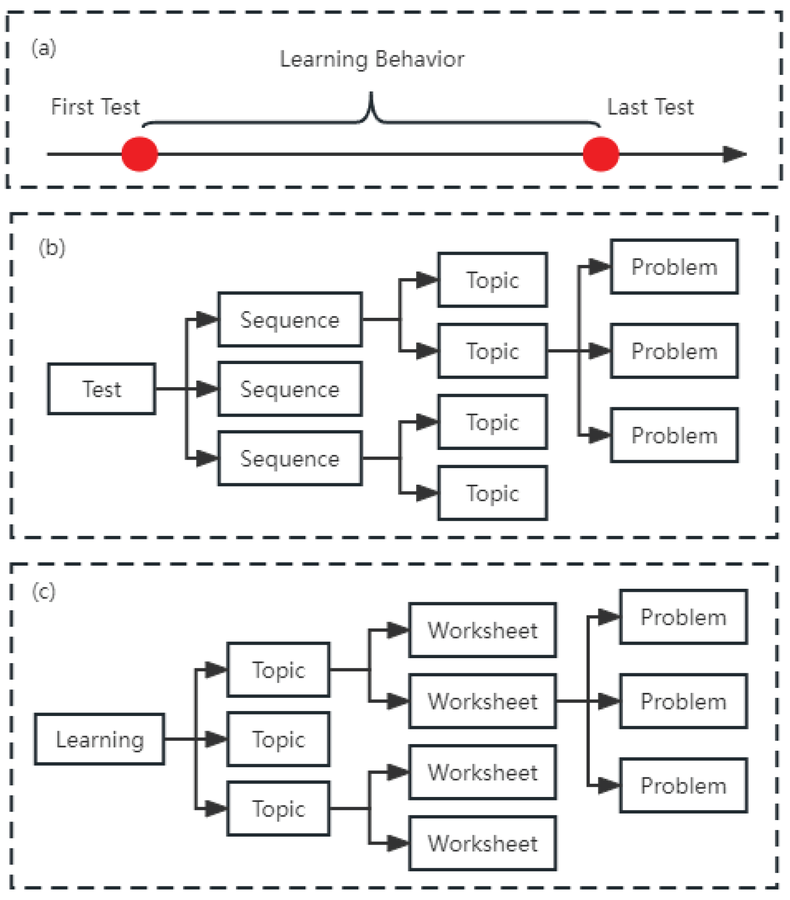
Figure 2.
Student Distribution in Speed vs. Hard-working.
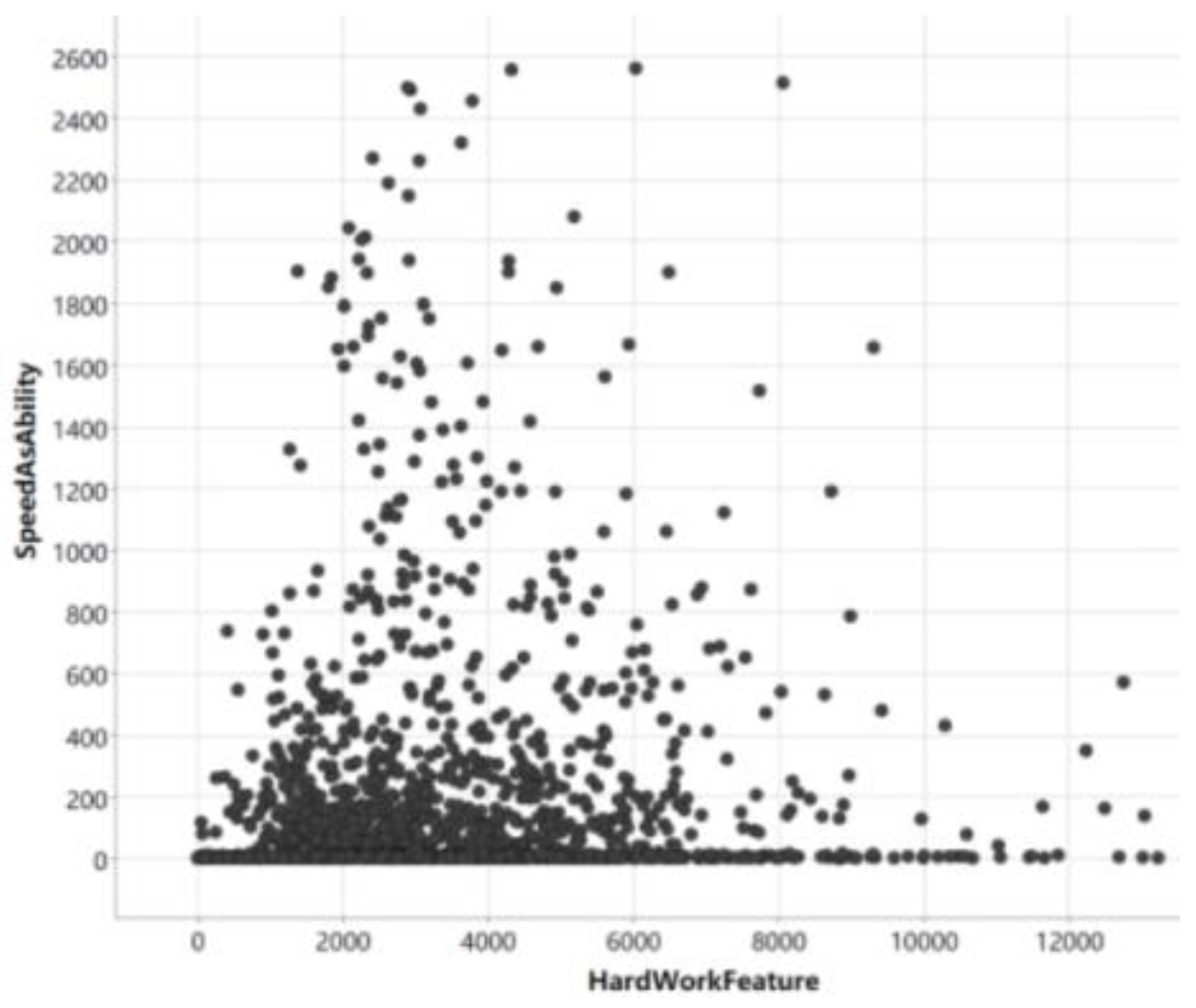
Figure 3.
Student Distribution in Speed vs. Accuracy.
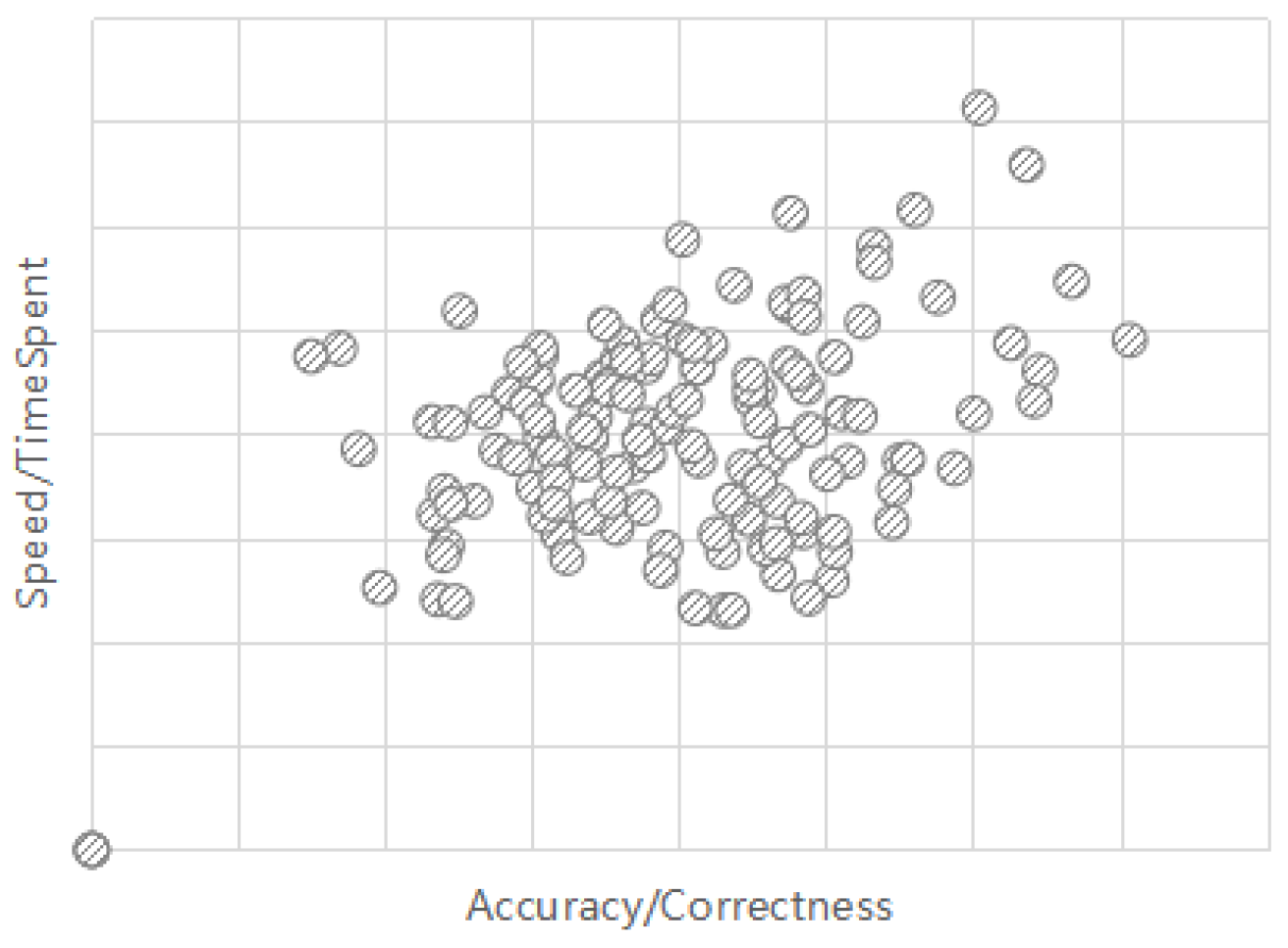
Figure 4.
Clustering Results and Student Counts. Silhouette Scores (b) Student Counts.
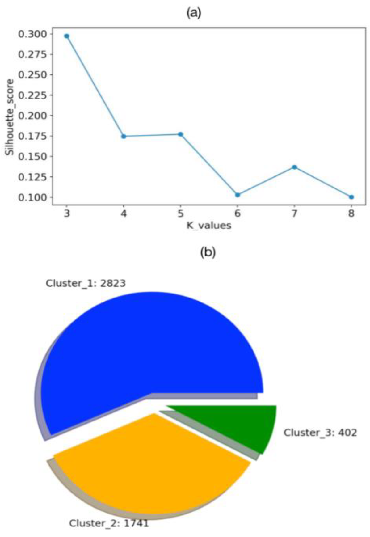
Figure 5.
Prediction Flowchart for “Learning beyond Test” Dataset.
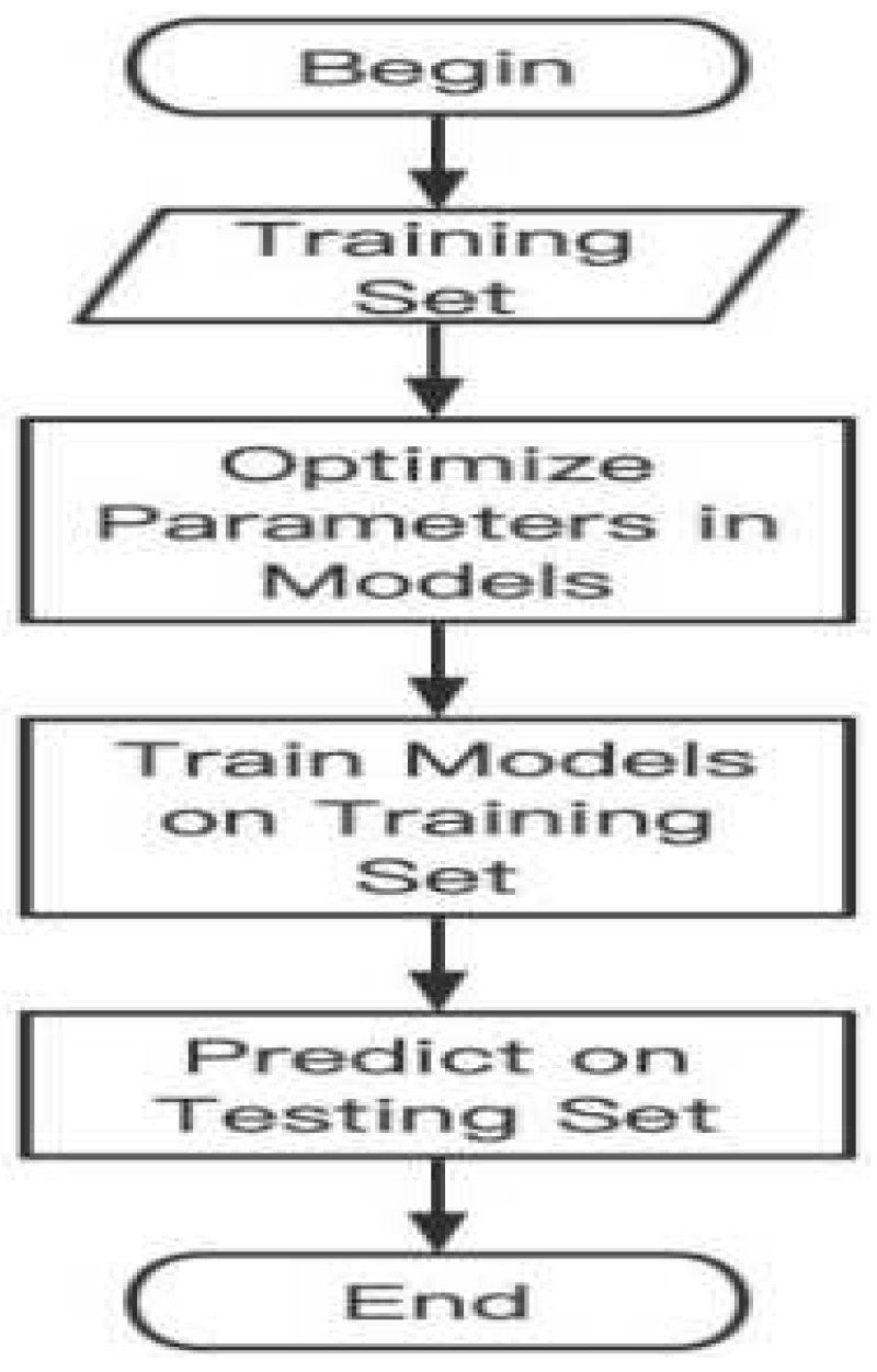
Figure 6.
Comparison of Difference Distributions in Subsets.
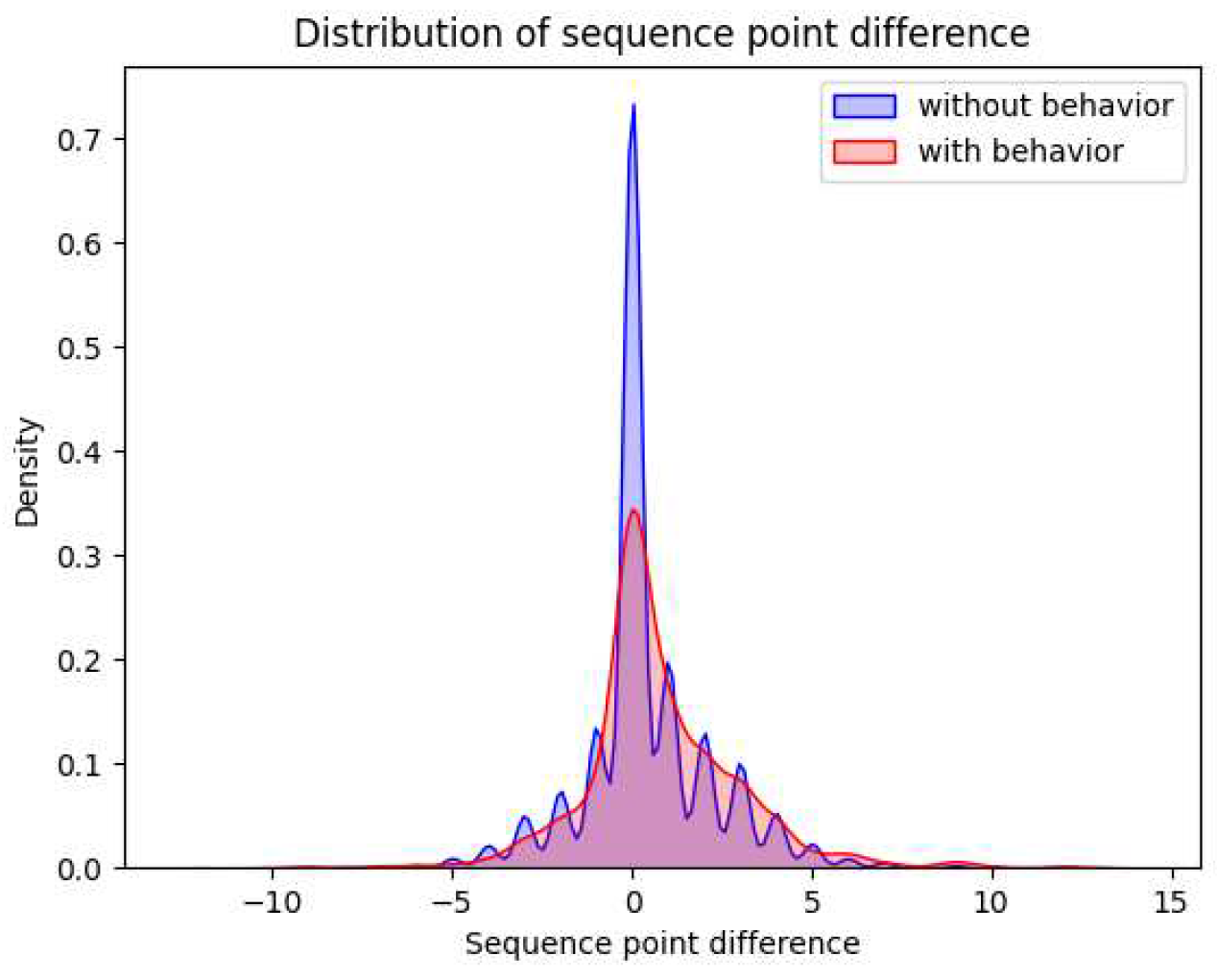
Figure 7.
Prediction Models for Students with and without Behavior Data.
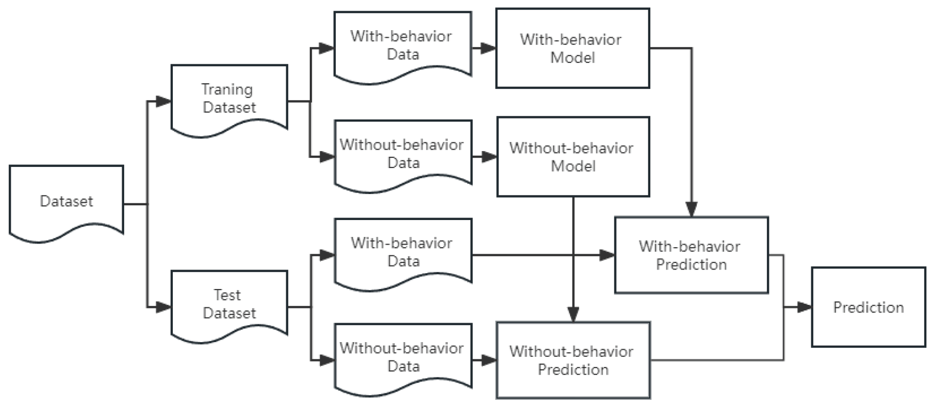
Figure 8.
Prediction Flowchart for “Learning with Test” Dataset.

Figure 9.
Mean MAE Values for Parameters at Various Levels.
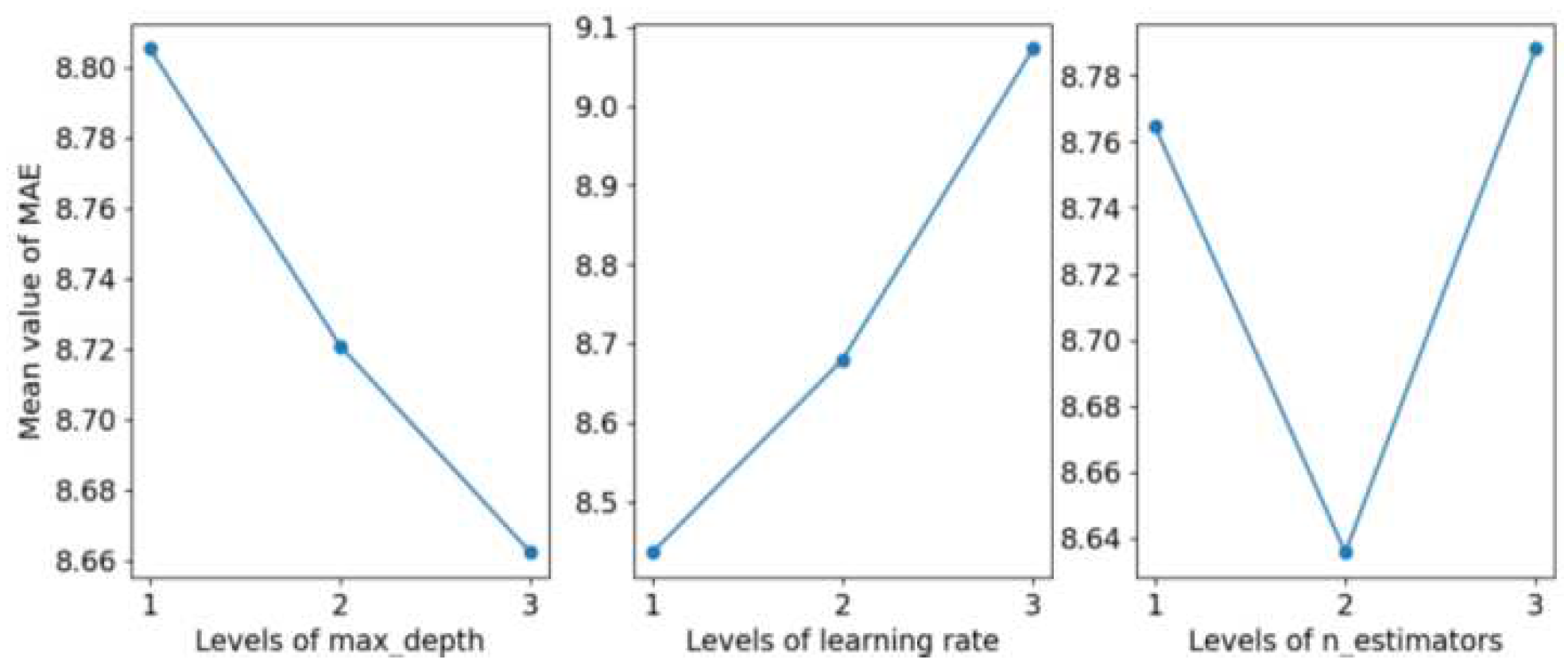
Figure 10.
CDF of Absolute Error in Averaged Correctness Prediction.

Figure 11.
CDF of Absolute Error in Averaged Timespent Prediction.
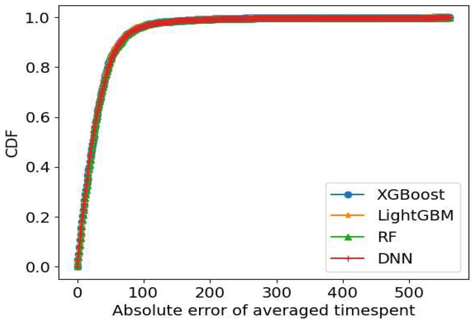
Table 1.
Dataset Comparison with Previous Studies.
| Dataset | Students | Period | Target | Accessibility |
| Kaur et al. (2015) | 152 | - | High school | private |
| Amrieh et al. (2016) |
500 | - | University | private |
| You (2016) |
530 | 15 weeks | University | private |
| Hamsa et al. (2016) | 168 | - | University | private |
| Saa (2016) | 270 | - | Higher education | private |
| Ha et al. (2020) | 525 | 2013-2016 | University | private |
| This work | 7,933 | 2010-2021 | Primary school | public |
Table 2.
Key Descriptors Derived from Raw Learning Data.
| Descriptor name | Construction method |
| numberOfTestsCompleted | count completed tests of each student |
| finishedCoursesNum | count the number of finished courses for each student |
| averagedEngagedTime | averaged value of engagedTime of each student |
| minEngagedTime | minimum value of engagedTime of each student |
| maxEngagedTime | maximum value of engagedTime of each student |
| averagedNumWorkAttempted | averaged value of numWorksheetsAttempted of each student |
| averagedNumProbCompleted | averaged value of numProblemsCompleted of each student |
| averagedNumNewlyMasteredTopics | averaged value of numNewlyMasteredTopics of each student |
| maxNumNewlyMasteredTopics | maximum value of numNewlyMasteredTopics of each student |
| averagedWastedTime | averaged value of wastedTime of each student |
| averagedNumProblemsCorrect | averaged value of numProblemsCorrect of each student |
| maxNumProblemsCorrect | max value of numProblemsCorrect of each student |
| minNumProblemsCorrect | min value of numProblemsCorrect of each student |
Table 3.
Primary Terms Used in the Dataset.
| Term | Grain | Description |
| studentID | Problem | ID of a student |
| sequenceID | Problem | ID of a sequence |
| topicID | Problem | ID of a topic |
| testNumProblems | Topic | Number of problems |
| testPercentCorrect | Topic | Correct percent |
| testTimespent | Topic | Spent time |
| testDateCompleted | Topic | Completed date |
| firstPoint | Sequence | Point in the first test |
| lastPoint | Sequence | Point in the last test |
| behNumProblems | Worksheet | Number of problems |
| behTimeLimit | Worksheet | Limitation of time |
| behNumRight | Worksheet | Number of right problems |
| behNumMissed | Worksheet | Number of missed problems |
| behNumSkipped | Worksheet | Number of skipped problems |
| behTimeSpent | Worksheet | Spent time |
| behDateCreated | Worksheet | Created date |
| behDateCompleted | Worksheet | Completed date |
Table 4.
Derived Features from the Original Data.
| Feature | Grain | Description |
| testTopicCnt | test | Count of topics |
| testProbAvgTime | test | Average spent time of problems |
| testAvgCorrectRate | test | Average correct rate of problems |
| behTopicCnt | behavior | Count of topics |
| behSheetCnt | behavior | Count of worksheets |
| behTopicAvgSheet | behavior | Average worksheets per topic |
| behTopicAvgTime | behavior | Average spent time per topic |
| behSheetAvgTime | behavior | Average spent time per worksheet |
| behProblemDone | behavior | Count of submitted problems |
| behNumRight | behavior | Count of right problems |
| behNumMissed | behavior | Count of missed problems |
| behProbAvgTime | behavior | Average spent time of problems |
| behAvgCorrectRate | behavior | Average correct rate of problems |
| behTopicDiff | behavior | behTopicCnt - testTopicCnt |
| behProbAvgTimeDiff | behavior | behProbAvgTime - testProbAvgTime |
| behCorrectRateDiff | behavior | behAvgCorrectRate - testAvgCorrectRate |
Table 5.
Comparison of Positive and Negative Segments with and without Behavior Data.
| Indicator | Without behavior | With behavior | P-value | ||
| Subset Part |
|||||
| Difference | Positive | Mean | 2.15 | 2.46 | 0.03 |
| Std. | 1.13 | 1.21 | 0.21 | ||
| Negative | Mean | -2.02 | -2.32 | 0.13 | |
| Std. | 1.10 | 1.04 | 0.37 |
Table 6.
Optimization Parameters and Their Ranges.
| Parameter | XGBoost | LightGBM | RF | DNN | Range |
| max_depth | √ | √ | √ | [3, 6, 9] | |
| learning rate | √ | √ | [0.1, 0.3, 0.5] | ||
| n_estimators | √ | √ | √ | [100, 300, 500] | |
| hidden_size | √ | [10, 50, 100] | |||
| max_iter | √ | [1000, 2500, 4000] |
Table 7.
Orthogonal Experimental Design and Evaluation Results for Parameters.
|
No. |
Max_depth | Learning rate | N_estimator | MAE |
| 1 | 3 (level 1) | 0.1 (level 1) | 100 (level 1) | 8.13 |
| 2 | 3 | 0.3 (level 2) | 300 (level 2) | 8.25 |
| 3 | 3 | 0.5 (level 3) | 500 (level 3) | 8.86 |
| 4 | 6 (level 2) | 0.1 | 300 | 7.86 |
| 5 | 6 | 0.3 | 500 | 8.18 |
| 6 | 6 | 0.5 | 100 | 8.64 |
| 7 | 9 (level 3) | 0.1 | 500 | 7.86 |
| 8 | 9 | 0.3 | 100 | 8.31 |
| 9 | 9 | 0.5 | 300 | 8.67 |
Table 8.
Optimal Parameter Values of the Models.
| Target | Model | Max_depth | Leaning_rate | N_estimator | Hidden_size | Max_iter |
| Averaged correctness prediction | XGBoost | 9 | 0.1 | 300 | - | - |
| LightGBM | 6 | 0.1 | 300 | - | - | |
| RF | 9 | - | 300 | - | - | |
| DNN | - | - | - | 100 | 2500 | |
| Averaged timespent prediction | XGBoost | 3 | 0.1 | 300 | - | - |
| LightGBM | 3 | 0.1 | 100 | - | - | |
| RF | 9 | - | 500 | - | - | |
| DNN | - | - | - | 100 | 2500 |
Table 9.
Comparison of the Prediction Results for Averaged Correctness.
| Training Set | Testing Set | |||||
| Model | MAE | RSME | R2 | MAE | RSME | R2 |
| XGBoost | 1.11 | 1.55 | 0.99 | 8.32 | 11.53 | 0.80 |
| LightGBM | 5.84 | 7.80 | 0.91 | 8.20 | 11.15 | 0.81 |
| RF | 5.48 | 7.12 | 0.92 | 8.46 | 11.54 | 0.80 |
| DNN | 8.62 | 11.45 | 0.80 | 9.78 | 12.89 | 0.74 |
Table 10.
Comparison of the Prediction Results for Timespent.
| Training set | Testing set | |||||
| Model | MAE | RSME | R2 | MAE | RSME | R2 |
| XGBoost | 21.97 | 29.75 | 0.70 | 31.28 | 46.34 | 0.23 |
| LightGBM | 29.87 | 43.27 | 0.36 | 31.27 | 45.68 | 0.26 |
| RF | 24.36 | 32.20 | 0.65 | 31.25 | 46.00 | 0.25 |
| DNN | 30.50 | 44.86 | 0.31 | 31.76 | 46.79 | 0.22 |
Table 11.
Prediction Results Comparison for Sequence Point.
| MAE | RMSE | R2 | |
| Baseline | 1.35 | 2.21 | 0.41 |
| Regression | 1.47 | 2.01 | 0.52 |
| GBRT | 1.33 | 1.92 | 0.56 |
Table 12.
The Coefficients of the Regression Models.
| Model | Rank | Feature | Coefficient |
| Without-behavior | 1 | firstPoint | 0.761 |
| 2 | testAvgCorrectRate | 0.417 | |
| With-behavior | 1 | firstPoint | 0.686 |
| 2 | behProbAvgTimeDiff | 3.189 | |
| 3 | behSheetAvgTime | -4.586 | |
| 4 | testTopicCnt | -0.359 | |
| 5 | testProbAvgTime | 1.728 | |
| 6 | behTopicAvgSheet | -1.866 | |
| 7 | behProblemDone | 0.722 | |
| 8 | behProbAvgTime | 2.102 | |
| 9 | behSheetCnt | -1.406 |
Table 13.
Comparison of the Prediction Results for Test Score.
| Model | Precision (weighted) |
Recall (weighted) |
F1-score (weighted) |
| Baseline | 0.542 | 0.736 | 0.624 |
| Regression | 0.666 | 0.711 | 0.677 |
| GBRT | 0.703 | 0.734 | 0.708 |
Disclaimer/Publisher’s Note: The statements, opinions and data contained in all publications are solely those of the individual author(s) and contributor(s) and not of MDPI and/or the editor(s). MDPI and/or the editor(s) disclaim responsibility for any injury to people or property resulting from any ideas, methods, instructions or products referred to in the content. |
© 2023 by the authors. Licensee MDPI, Basel, Switzerland. This article is an open access article distributed under the terms and conditions of the Creative Commons Attribution (CC BY) license (http://creativecommons.org/licenses/by/4.0/).
Copyright: This open access article is published under a Creative Commons CC BY 4.0 license, which permit the free download, distribution, and reuse, provided that the author and preprint are cited in any reuse.
MDPI Initiatives
Important Links
© 2024 MDPI (Basel, Switzerland) unless otherwise stated


