1. Introduction
Spatial interpolation is a fundamental technique employed in spatial data analysis to estimate the variable of interest at unobserved locations based on available data. Kriging is a geostatistical approach for spatial interpolation that provides a best linear unbiased prediction with the minimum estimation variance. An approximation of the kriging models relies on the assumption that a random process can be decomposed into a trend function and a random residual component. Ordinary kriging (OK) is a commonly used method with a constant trend, which is not suitable in the presence of a strong trend structure. On the other hand, kriging with external drift (KED) allows for the inclusion of auxiliary variables that have a strong spatial correlation with the target variable in order to increase precision in estimates [
1,
2]. In the KED, a trend model that is fitted to both target data points and significant auxiliary samples is first generated. The empirical variogram is thereafter derived from residuals computed from the difference between the trend estimates and measured values. A final prediction of the target variable is obtained as a weighted linear combination of observations, in which the weights are calculated through the Lagrange multiplier method. The KED method has been applied in various fields, including meteorology [
3,
4,
5,
6], geology [
7,
8,
9,
10], environmental modeling [
11,
12,
13], agronomy [
14,
15,
16], and hydrology [
17].
The trend term for the KED is conventionally modelled by polynomial functions of degree one or two. However, in practice, a non-linear relationship often exists between influence factors and response variables where the application of such a polynomial is not adequate. Despite extensive research on the prediction using KED having been conducted, a study of non-linear trend functions for the KED remains scarce. Snepvangers et al. [
18] developed a non-linear trend represented by a logarithmic function to interpolate soil water content using the KED technique with net-precipitation as an auxiliary variable. Freier and Lieres [
19] introduced a novel extension to universal kriging (UK), a specific instance of KED, aimed at handling non-linear trend patterns. They utilized a Taylor-based linearization approach in conjunction with an iterative parameter estimation procedure to construct a non-linear trend model. The method was applied to the Michaelis-Menten equation, which describes an enzymatic reaction. Freier et al. [
20] subsequently employed this kriging technique to interpolate biocatalytic data with low and irregular density. Their method can be particularly of use in the presence of an explicit expression of the non-linear trend functions. Nevertheless, an interaction between design factors and system response in real-world applications is naturally described by diverse and complex behaviour, which is difficult to establish in an explicit form.
Machine learning (ML) has recently been gaining attention as a computationally efficient tool for identifying implicit relationships between variables. This allows one to generate and optimize the complex model based on the huge amount of data available for analysis. Support vector machine (SVM) is a kernel-based machine learning approach used for classification and regression. The particular use of SVMs for regression problems is called support vector regression (SVR), which was first introduced by Vapnik in 1992 [
21]. The method adopts the structural risk minimization principle by minimizing the upper bound of the generalization errors. This leads to a linear decision function, which is essentially a convex quadratic programming (QP) problem. The core element of SVR is to search for the optimal hyperplane that fits the learning data while maximizing the distance between the hyperplane and the data points. In the case of non-linear problems, the SVR procedure starts by projecting input data into high-dimensional feature space through some non-linear mapping, and the SVR subsequently performs linear regression to obtain the optimal hyperplane. Apart from producing high prediction accuracy for non-linear data, SVR is also suitable for applications characterized by small datasets [
22,
23,
24]. Furthermore, this SVM regression-based algorithm has the generalization ability to reduce overfitting issues by introducing regularization term into the loss function. Due to all these advantages, the technique has therefore been applied in diverse disciplines, including finance [
25,
26], economics [
27,
28], climate modelling [
29,
30], and healthcare [
31,
32]. However, SVR requires substantial computational time and significant memory usage to solve the QP problem. To overcome these limitations, Suykens and Vandewalle [
33] proposed a variant of SVR known as least squares support vector regression (LSSVR). This method extends the traditional SVR by using a squared loss function rather than quadratic programming. The LSSVR results yield higher accuracy and require less computational resources compared to the reliability method relying on SVR [
34].
There is a notable absence of research on the utilization of ML in geostatistical techniques. In this work, we will present a novel interpolation method in which the LSSVR method is used to compute non-linear trend functions within the context of KED. The proposed technique entails expressing the trend function in a structured form through explicit feature mapping. The purpose of our technique is to enhance the predictive capabilities of the KED model by incorporating the powerful capabilities of LSSVR for capturing non-linear relationships between variables.
The remainder of this paper is outlined as follows.
Section 2 reviews the theory regarding the KED methodology and LSSVR technique. A detailed description of the KED using the LSSVR for modelling the non-linear trend functions is provided in
Section 3. In
Section 4, we conduct a comparative simulation study using the conventional KED model and the proposed method for temperature and pressure estimation in Thailand. Conclusion and discussion are drawn in
Section 5.
2. Mathematical Background
2.1. Kriging with External Drift
Kriging is a spatial interpolation method that uses variogram analysis to predict the variable of interest at an unmeasured location based on the values of surrounding measured locations. It is the best linear unbiased estimator (BLUE) for the random function,
, where
D is a defined spatial domain and
d a positive integer representing the number of dimensions in the spatial domain. The value of
can be obtained through
where a deterministic component
indicates the underlying trend or drift and
is a stochastic residual component with a mean of zero and a variogram, which is a function of lag vector [
2].
In KED, the trend is modelled by a function of auxiliary variables which can be expressed as
where
is coefficient to be estimated,
is prescribed function that maps from the domain
D into the range
, and
is the number of terms used in the approximation. Additionally, the function
is defined to be 1 for all
s in
D [
2].
To determine the unknown coefficients in equation (
2), we can use the ordinary least squares (OLS) estimator or its extension, the generalized least squares (GLS) estimator, which accounts for the spatial correlation between individual observations [
35].
Given
n observed values,
, at sample points,
. The attribute
at an ungauged site
is estimated as a linear combination of observed values so that
where
is the kriging weight assigned to
. The weights
are computed by minimizing the estimation error variance subject to the unbiased constraint. This results in the following optimization problem:
The optimal weights of the system (
4) for the KED model can be solved by using the Lagrange multiplier method which leads to
where
denotes the residual variogram function of
and
is a Lagrange multiplier.
The variogram is a fundamental and important tool that quantifies the spatial correlation structure of the sample points. The variogram model is a smooth function that is reasonably well fitted to the empirical variogram estimated from the data. In the present study, we use the empirical variogram estimator introduced by Matheron [
36], and the parametric variogram is represented by an exponential model [
35].
In general, both linear and quadratic functions are usually treated as a trend representation [
9,
17,
37,
38]. However, in certain scenarios, the relationship between the target and auxiliary variables is too complex to be captured by simple polynomial functions. In this work, least squares support vector regression (LSSVR) is used to model a non-linear trend function within the KED framework.
2.2. Least Squares Support Vector Regression
Given a dataset
, where
is a
dimensional training data point and
represents a target output. The objective of least squares support vector regression (LSSVR) is to find a function that minimizes the square error between the predicted values and the actual values. In LSSVR, the input data
are mapped into a higher-dimensional feature space
, in which a linear model is adopted, so that a model function
is formulated as
where
is an
dimensional feature mapping,
is an
weight vector, and
indicates a bias term.
In equation (
6), the unknown vector
and parameter
b can be calculated by solving the following optimization problem:
where
is a regularization constant that constitutes a trade-off between the model complexity and the empirical error, and
is a regression error.
The problem (
7) can be reformulated as an unconstrained problem through the Lagrange multiplier method [
39]. A set of linear equations corresponding to optimality conditions is consequently obtained, which provides an expression of the weight vector
:
where
is a Lagrange multiplier. This system of equations can be reduced to the following form:
where
is referred to as the kernel matrix whose element is
for
and
is the identity matrix of size
n. The matrix
is an
unit matrix and
is the
matrix of observed values together with the
matrix of Lagrange multipliers,
.
The solutions of equation (
9) are
where
, which is a symmetric and positive semi-definite matrix, thereby ascertaining the existence of its inverse, denoted as
.
By replacing equation (
8) with equation (
6), the model for the LSSVR function therefore becomes
where
is the kernel associated with the feature mapping
, and it is defined as [
40]
Numerous kernel functions are available for the construction of various models, such as:
Linear kernel: .
Polynomial kernel: , and .
Radial basis function kernel: , and means the Euclidean norm.
The LSSVR regarding the KED scheme is used to characterize the underlying trend. The notation for the dataset at the sample point is represented by , where is the vector of auxiliary variables and denotes the observation value.
3. A Novel Trend Function of KED based on LSSVR
This section introduces a method for constructing the trend function in KED using the LSSVR method. The approach involves identifying the fundamental functions of the trend through explicit feature mapping. Examples of explicit feature mappings derived from the corresponding kernel functions are also demonstrated.
3.1. Construction of the Trend Function
Let
be an
dimensional feature mapping such that
where
is the
mth component of the feature mapping.
According to equation (
13), the kernel function is in the form:
By substituting equation (
15) into equation (
12),
can be rewritten as
The trend function can hence be written in the following form:
where the coefficient
and
is the known function for
in which
and
.
Equation (
17) possesses a similar form to equation (
2) with
being treated as
and
being
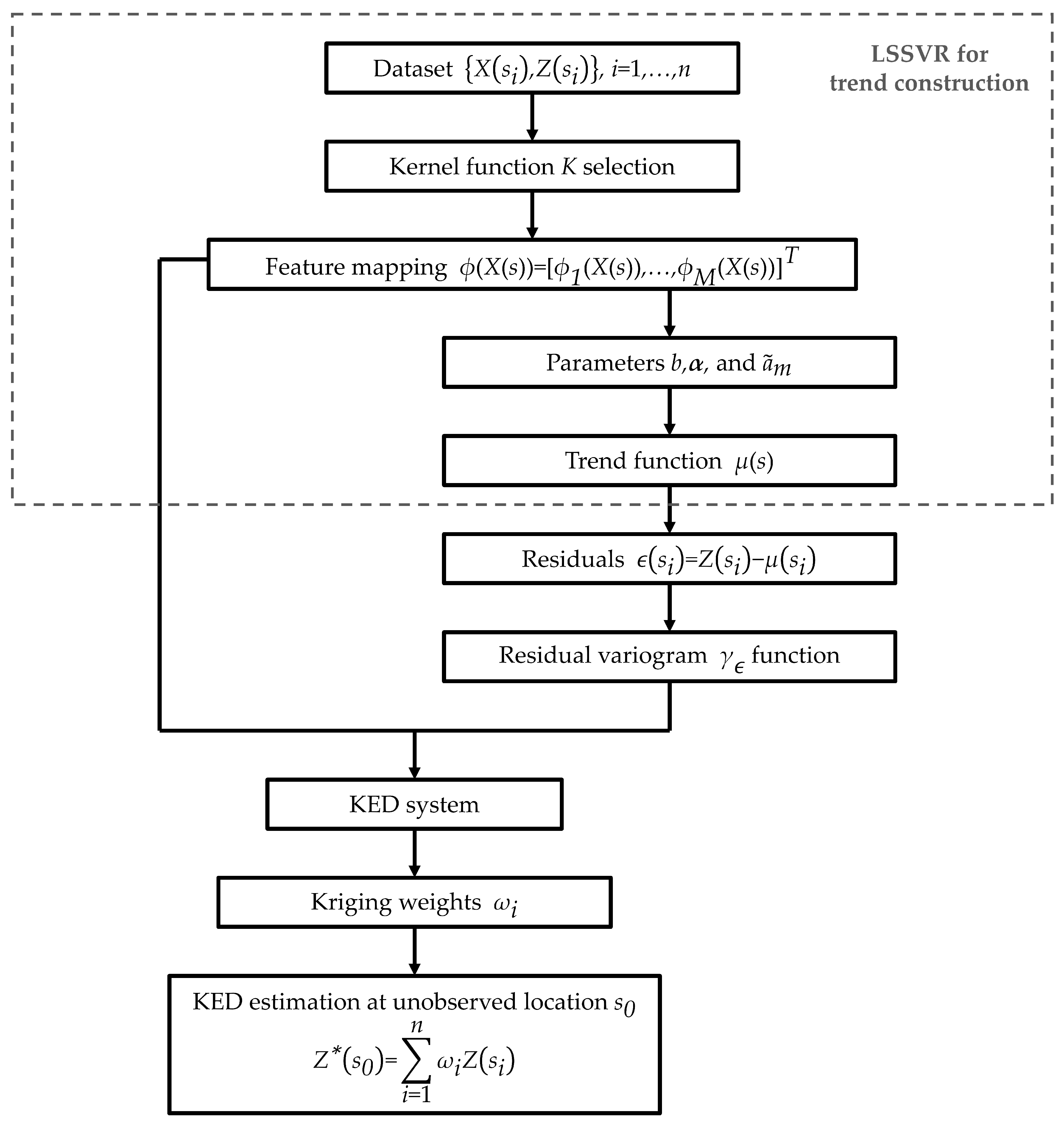
. This verifies the use of the kernel function as a non-linear trend model for the KED. The process of the KED based on the LSSVR method is provided according to the flowchart shown in
Figure 1.
3.2. Examples of Explicitly Feature Mapping
There have been various kernels for the LSSVR method, namely linear, polynomial, and radial basis function kernels [
41,
42,
43]. This section presents the last two kernels, as they are widely used and relatively easy to tune. They will also be applied in our model to formulate the trend component.
3.2.1. Polynomial Kernel
The polynomial kernel function is defined as
where
and
is the degree of polynomial.
The feature mapping for polynomial kernel degree
is given by [
44]
where the dimensionality of
is
[
45]. For example, when the degree of the polynomial kernel and the number of auxiliary variables are both equal to 2, with
k being 1, then
Comparing with equation (
14), components of the feature mapping are as follows:
, , ,
, , .
3.2.2. Radial Basis Function Kernel
The implicit kernel function, exemplified by the radial basis function (RBF) kernel, assumes the following form:
where
is a RBF kernel parameter.
The feature mapping for RBF kernel function can be formulated as
where
which is described in more detail in [
46]. The RBF kernel function, which maps the auxiliary data to an infinite−dimensional space, can be approximated by Taylor Polynomial-based Monomial feature mapping (TPM feature mapping). In the work of [
46], a finite-dimensional approximated feature mapping of the RBF function is obtained as follows:
where
is a selected approximation degree and the TPM feature mapping degree
has
dimensions.
Although an increase in
leads to an improvement in estimation as
approaches the true function, it is however sufficient enough to use the TPM feature mapping with low dimensions [
46]. An example of TPM feature mapping with degree−two and 2 auxiliary variables is
By comparing equation (
25) with equation (
14), this results in
, ,
, ,
, .
4. Case Study: Estimations of Temperature and Pressure in Thailand
4.1. Study Area
The evaluation of the efficiency and accuracy of the proposed techniques was carried out to interpolate temperature and pressure in Thailand. The country is located between
N and
N latitude and
E and
E longitude, with a total area of 513,115
and a coastline of 3,219
[
47,
48]. The data used in this study consist of monthly averages of temperature, pressure, relative humidity, digital elevation model (DEM), and geographic locations (coordinates) spanning from January 2017 to December 2017. These data were acquired from the National Hydroinformatics and Climate Data Center (NHC), developed by Hydro-Informatics Institute (HII) [
49].
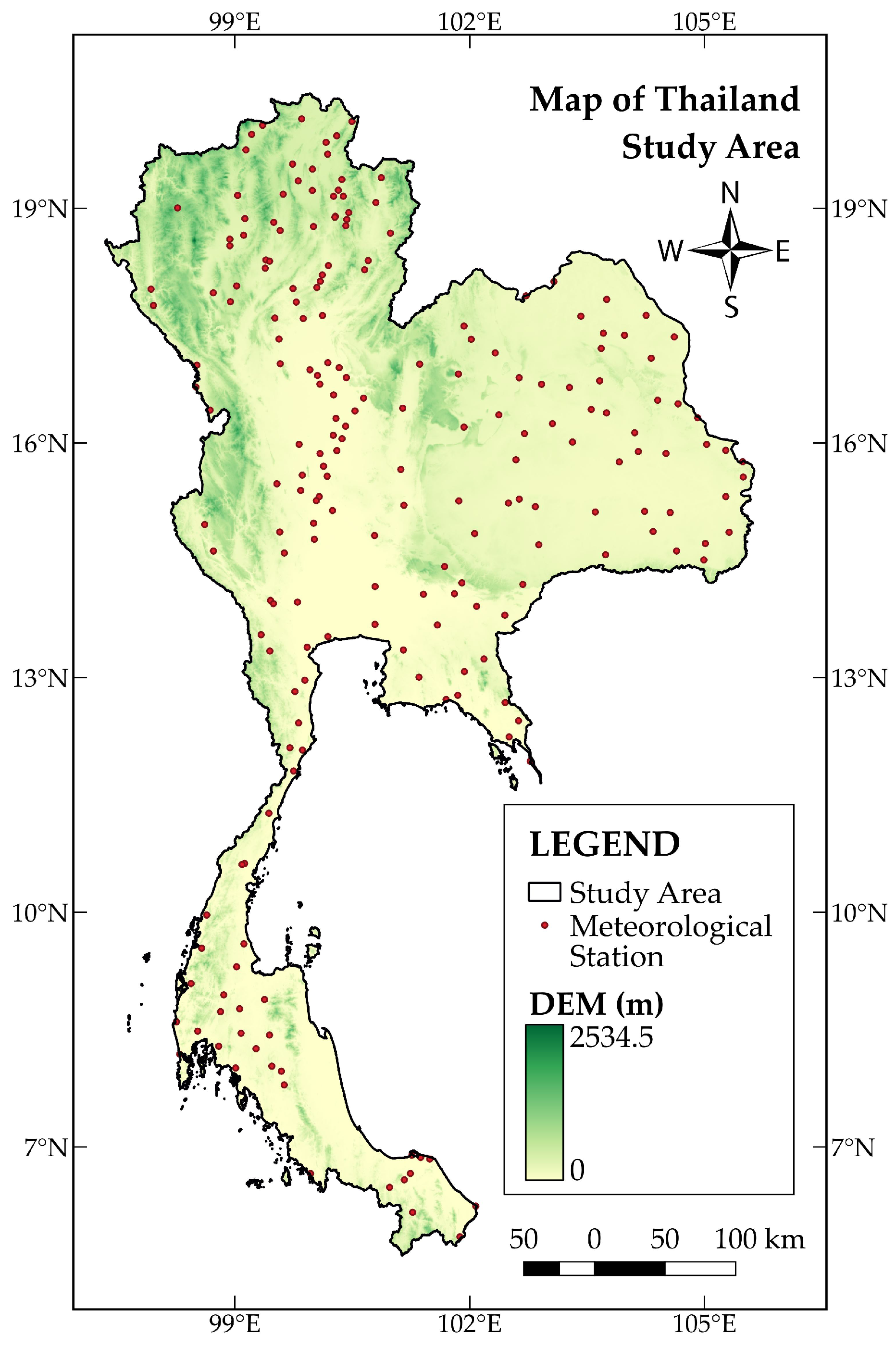
Figure 2 displays 213 meteorological stations after data preparation and cleaning.
4.2. Evaluation of Model Accuracy
In this study, we compare the accuracy of KED with three different trend functions: the linear trend function estimated using the GLS estimator (KED−GLS), the non-linear trend function based on LSSVR with polynomial feature mapping of degree one and two (KED−Poly1 and KED−Poly2), and the non-linear trend function based on LSSVR with TPM feature mapping of degree one and two (KED−TPM1 and KED−TPM2).
The
fold cross-validation technique was applied to examine the performance of the models. The data were randomly divided into 10 folds. For each iteration, each fold was used as a testing dataset for the model built upon the remaining nine folds. After 10 iterations in which each fold was once selected as testing data, the overall estimation accuracy is an average of the accuracy scores calculated from each iteration [
50]. The root-mean-square error (RMSE) [
51] and the mean-absolute-percentage error (MAPE) [
52] were the model performance indicators, which are formulated as follows:
where
N is the number of observations,
and
denote the observed data and the estimated value at coordinate
, respectively.
4.3. Results
Before proceeding to the KED simulation, a selection of auxiliary factors is required.
Table 1 presents the statistical analysis of the interdependence between each selected variable and the target variables through the Pearson and Spearman correlation coefficients [
53]. The results indicate a significant positive correlation between temperature and pressure (correlation coefficients greater than 0.5). While the pressure is negatively correlated to both DEM and latitude with the correlation coefficients less than -0.5. This suggests that pressure can be chosen as an auxiliary variable for temperature estimation and vice versa. On the other hand, both DEM and latitude are additionally included as auxiliary factors for interpolating pressure.
Table 2 reports the estimation efficiency of the KED model with three different trend functions via MAPE and RMSE measures. According to the accuracy statistics, the KED with a non-linear trend function based on LSSVR has a superior estimation performance to that of the KED with a linear trend for both temperature and pressure. Specifically, the prediction errors for temperature generated by the KED−TPM2 are smaller than those of all other methods, with RMSE being 0.8123 and MAPE being 2.2888. These are respectively equivalent to 1.5633% and 2.1755% improvement compared to the KED−GLS method. While the optimal pressure estimates are achieved by using the KED−Poly2 with the RMSE and MAPE equal to 7.7541 and 0.5466 respectively. The KED−Poly2 reduces both MAPE and RMSE values by over 10% with respect to the KED−GLS approach.
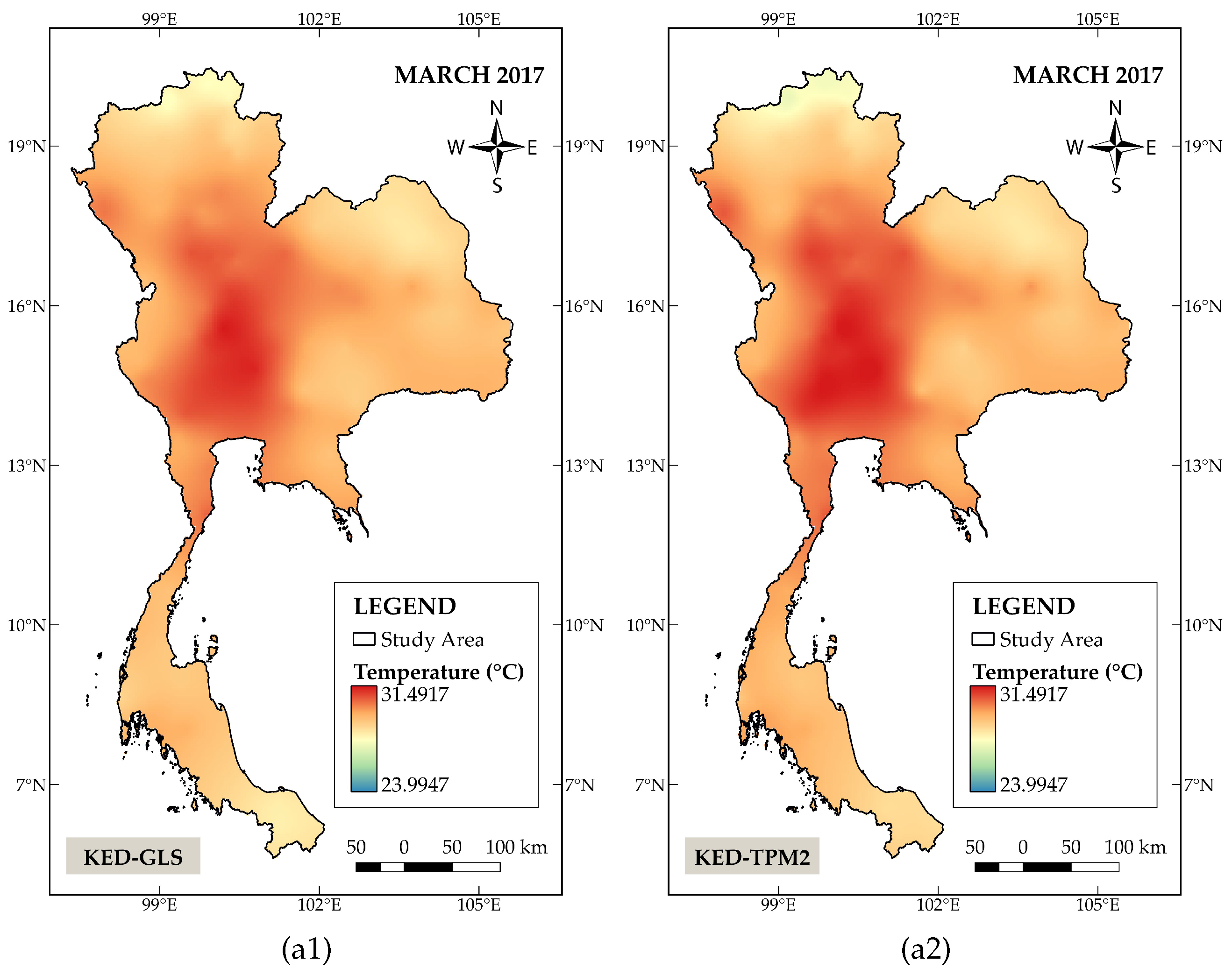
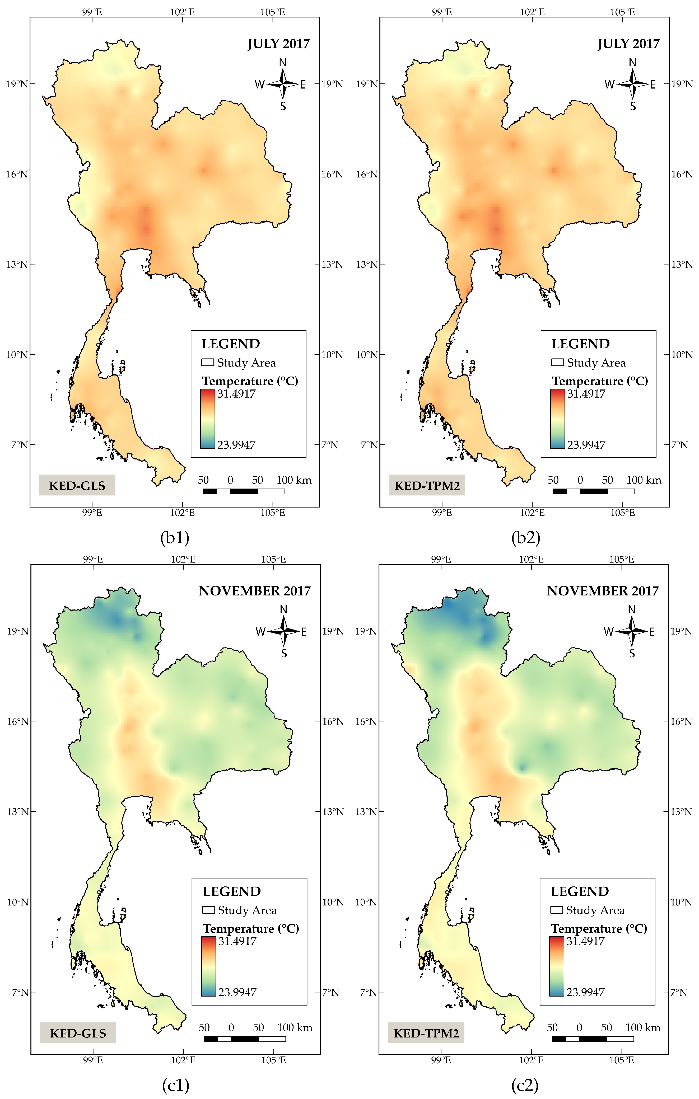
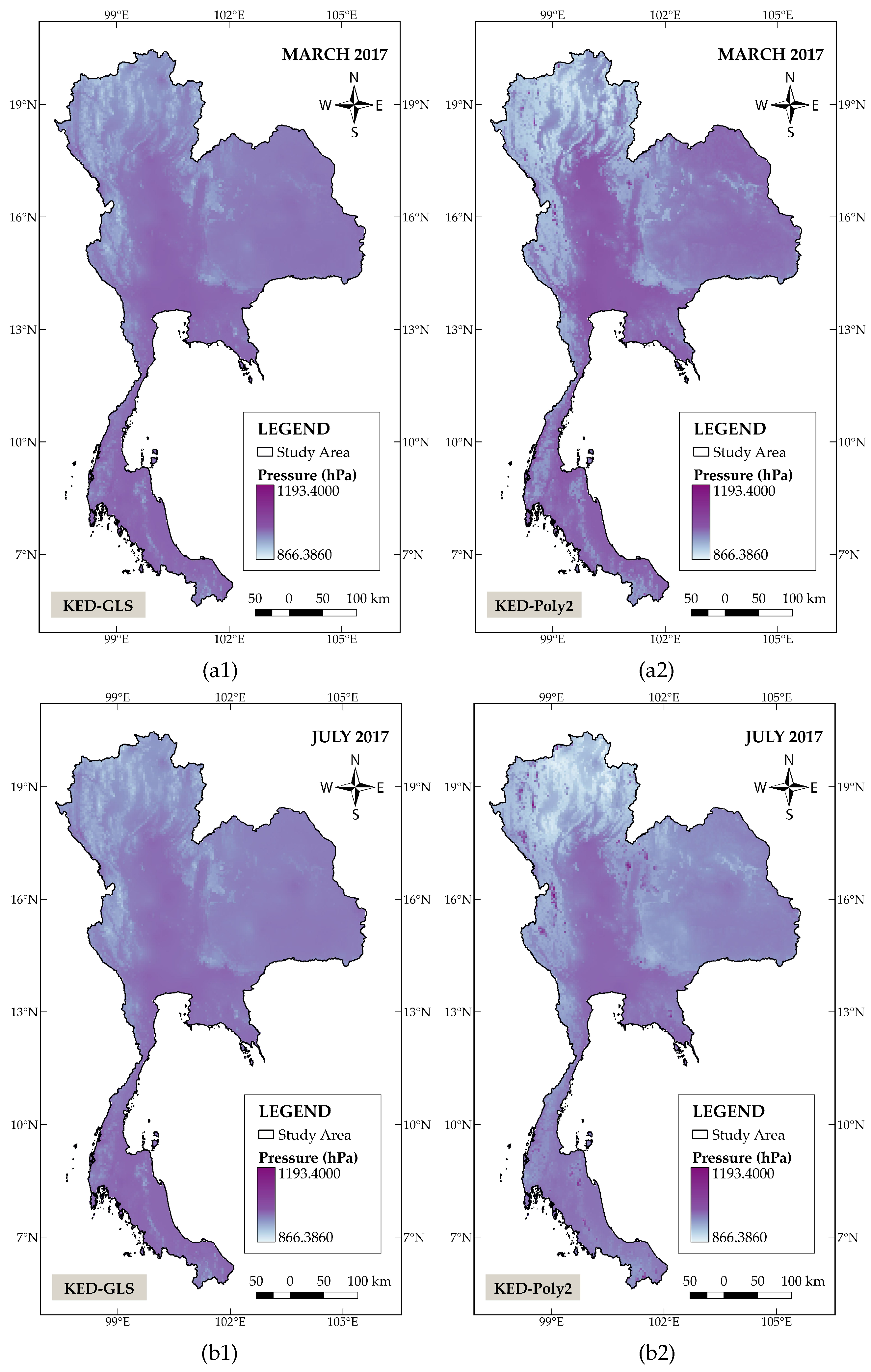
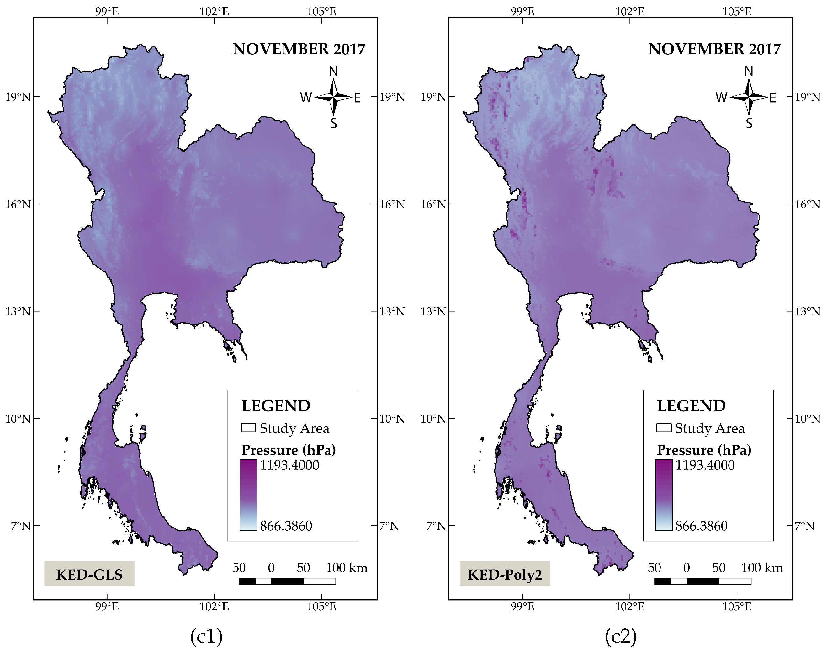
To further compare the estimation performance of all methods, visual spatial distribution patterns of the monthly averages of temperature and pressure in Thailand in March, July, and November 2017 are presented. These maps were created using QGIS (Quantum Geographic Information System) software and the study area was partitioned into a grid of square cells of 0.05 degree per side.
Figure 3 shows the spatial distribution patterns of the monthly mean temperature. The panels on the left column depict the results generated by KED−GLS, whereas panels on the right column illustrate the results obtained from KED−TPM2. Both KED−TPM2 and KED−GLS produce a roughly similar distribution pattern for the average July temperature. This may be due to the fact that there is a small variation in temperature across the country during the rainy season (July-October). The discrepancy in temperature derived from these two models is therefore not significant. On the contrary, clear differences can be observed in March and November, in which the area of high temperature is more broadly distributed in the central part of the country for the KED−TPM2. The model also generates an overall lower temperature level concentrated in the northern region in November.
Figure 4displays spatial distribution maps of monthly mean pressure where the left column again corresponds to the estimates attained from the KED−GLS while those in the right column are derived from the KED−Poly2. The results show a distinct difference between these two methods. In particular, lower pressure values estimated by KED−Poly2 are clearly marked in the northern and western parts of the study area.
5. Conclusion and Discussion
This paper presents the novel KED method that applies the LSSVR technique to improve spatial interpolation accuracy in the presence of non-linear trends. The method involves determining the drift component through explicit feature mapping which is expressed in terms of kernel functions. A comparison between our proposed method and the KED with the linear trend is demonstrated in the case of the temperature and pressure estimation in Thailand in 2017. The results show that the KED with LSSVR outperforms the KED approach with a linear trend function regarding estimation accuracy.
The advantage of the KED with LSSVR can be attributed to its ability to extract implicit non-linear relationships between the target and auxiliary variables. This gives rise to more accurate interpolation results. Furthermore, the LSSVR is a powerful machine learning algorithm that has been proven effective in a variety of regression tasks. This allows our method to adapt to various data types. However, the choice of kernel function in LSSVR can have a significant impact on the estimation accuracy. Although a higher-degree polynomial kernel or a higher-degree TPM feature mapping can model more complex relationships in the data, it can also result in a number of equations in the kriging system. This can lead to more time-intensive computation and an increase in the likelihood of model overfitting issues.
Author Contributions
Conceptualization, K.B., N.C. and S.M.; methodology, K.B., N.C. and S.M.; software, K.B. and S.M.; validation, K.B., N.C. and S.M.; formal analysis, K.B., N.C., and S.M.; investigation, K.B., N.C. and S.M.; resources, K.B., N.C. and S.M.; data curation, K.B. and S.M.; writing-original draft preparation, K.B., N.C. and S.M.; writing-review and editing, K.B., N.C. and S.M.; visualization, K.B.; supervision, N.C. and S.M. All authors have read and agreed to the published version of the manuscript.
Data Availability Statement
All data were acquired from the National Hydroinformatics and Climate Data Center (NHC), developed by Hydro-Informatics Institute (HII) [
49].
Acknowledgments
This work was supported by (i) Chiang Mai University (CMU) and (ii) a Fundamental Fund provided by Thailand Science Research and Innovation (TSRI) and National Science, Research and Innovation Fund (NSRF).
Conflicts of Interest
The authors declare no conflict of interest.
References
- Wackernagel, H. Multivariate geostatistics: an introduction with applications; Springer Science & Business Media, 2003. [Google Scholar]
- Webster, R.; Oliver, M.A. Geostatistics for environmental scientists; John Wiley & Sons, 2007. [Google Scholar]
- Hudson, G.; Wackernagel, H. Mapping temperature using kriging with external drift: theory and an example from Scotland. International journal of Climatology 1994, 14, 77–91. [Google Scholar] [CrossRef]
- Bostan, P.; Heuvelink, G.B.; Akyurek, S. Comparison of regression and kriging techniques for mapping the average annual precipitation of Turkey. International Journal of Applied Earth Observation and Geoinformation 2012, 19, 115–126. [Google Scholar] [CrossRef]
- Varentsov, M.; Esau, I.; Wolf, T. High-resolution temperature mapping by geostatistical kriging with external drift from large-eddy simulations. Monthly Weather Review 2020, 148, 1029–1048. [Google Scholar] [CrossRef]
- Cantet, P. Mapping the mean monthly precipitation of a small island using kriging with external drifts. Theoretical and Applied Climatology 2017, 127, 31–44. [Google Scholar] [CrossRef]
- Bourennane, H.; King, D.; Chery, P.; Bruand, A. Improving the kriging of a soil variable using slope gradient as external drift. European Journal of Soil Science 1996, 47, 473–483. [Google Scholar] [CrossRef]
- Bourennane, H.; King, D.; Couturier, A. Comparison of kriging with external drift and simple linear regression for predicting soil horizon thickness with different sample densities. Geoderma 2000, 97, 255–271. [Google Scholar] [CrossRef]
- Bourennane, H.; King, D. Using multiple external drifts to estimate a soil variable. Geoderma 2003, 114, 1–18. [Google Scholar] [CrossRef]
- Béjar-Pizarro, M.; Guardiola-Albert, C.; García-Cárdenas, R.P.; Herrera, G.; Barra, A.; López Molina, A.; Tessitore, S.; Staller, A.; Ortega-Becerril, J.A.; García-García, R.P. Interpolation of GPS and geological data using InSAR deformation maps: Method and application to land subsidence in the alto guadalentín aquifer (SE Spain). Remote Sensing 2016, 8, 965. [Google Scholar] [CrossRef]
- Beauchamp, M.; de Fouquet, C.; Malherbe, L. Dealing with non-stationarity through explanatory variables in kriging-based air quality maps. Spatial statistics 2017, 22, 18–46. [Google Scholar] [CrossRef]
- Beauchamp, M.; Malherbe, L.; de Fouquet, C.; Létinois, L.; Tognet, F. A polynomial approximation of the traffic contributions for kriging-based interpolation of urban air quality model. Environmental Modelling & Software 2018, 105, 132–152. [Google Scholar] [CrossRef]
- Troisi, S.; Fallico, C.; Straface, S.; Migliari, E. Application of kriging with external drift to estimate hydraulic conductivity from electrical-resistivity data in unconsolidated deposits near Montalto Uffugo, Italy. Hydrogeology Journal 2000, 8, 356–367. [Google Scholar] [CrossRef]
- Garcia-Papani, F.; Leiva, V.; Ruggeri, F.; Uribe-Opazo, M.A. Kriging with external drift in a Birnbaum–Saunders geostatistical model. Stochastic Environmental Research and Risk Assessment 2018, 32, 1517–1530. [Google Scholar] [CrossRef]
- Cafarelli, B.; Castrignanò, A. The use of geoadditive models to estimate the spatial distribution of grain weight in an agronomic field: a comparison with kriging with external drift. Environmetrics 2011, 22, 769–780. [Google Scholar] [CrossRef]
- Anand, A.; Singh, P.; Srivastava, P.K.; Gupta, M. GIS-based analysis for soil moisture estimation via kriging with external drift. In Agricultural water management; Elsevier, 2021; pp. 391–408. [Google Scholar] [CrossRef]
- Rivest, M.; Marcotte, D.; Pasquier, P. Hydraulic head field estimation using kriging with an external drift: A way to consider conceptual model information. Journal of Hydrology 2008, 361, 349–361. [Google Scholar] [CrossRef]
- Snepvangers, J.; Heuvelink, G.; Huisman, J. Soil water content interpolation using spatio-temporal kriging with external drift. Geoderma 2003, 112, 253–271. [Google Scholar] [CrossRef]
- Freier, L.; von Lieres, E. Kriging based iterative parameter estimation procedure for biotechnology applications with nonlinear trend functions. IFAC-PapersOnLine 2015, 48, 574–579. [Google Scholar] [CrossRef]
- Freier, L.; Wiechert, W.; von Lieres, E. Kriging with trend functions nonlinear in their parameters: Theory and application in enzyme kinetics. Engineering in life sciences 2017, 17, 916–922. [Google Scholar] [CrossRef] [PubMed]
- Mozer, M.C.; Jordan, M.I.; Petsche, T. Advances in Neural Information Processing Systems 9: Proceedings of the 1996 Conference; Mit Press, 1997; Volume 9. [Google Scholar]
- Al-Anazi, A.F.; Gates, I.D. Support vector regression to predict porosity and permeability: Effect of sample size. Computers & geosciences 2012, 39, 64–76. [Google Scholar] [CrossRef]
- Wiering, M.A.; Van der Ree, M.H.; Embrechts, M.; Stollenga, M.; Meijster, A.; Nolte, A.; Schomaker, L. The neural support vector machine. BNAIC 2013: Proceedings of the 25th Benelux Conference on Artificial Intelligence, Delft, The Netherlands, November 7-8, 2013. Delft University of Technology (TU Delft); under the auspices of the Benelux …, 2013.
- Zhong, H.; Wang, J.; Jia, H.; Mu, Y.; Lv, S. Vector field-based support vector regression for building energy consumption prediction. Applied Energy 2019, 242, 403–414. [Google Scholar] [CrossRef]
- Henrique, B.M.; Sobreiro, V.A.; Kimura, H. Stock price prediction using support vector regression on daily and up to the minute prices. The Journal of finance and data science 2018, 4, 183–201. [Google Scholar] [CrossRef]
- Zhang, J.; Teng, Y.F.; Chen, W. Support vector regression with modified firefly algorithm for stock price forecasting. Applied Intelligence 2019, 49, 1658–1674. [Google Scholar] [CrossRef]
- Mishra, S.; Padhy, S. An efficient portfolio construction model using stock price predicted by support vector regression. The North American Journal of Economics and Finance 2019, 50, 101027. [Google Scholar] [CrossRef]
- Fan, G.F.; Yu, M.; Dong, S.Q.; Yeh, Y.H.; Hong, W.C. Forecasting short-term electricity load using hybrid support vector regression with grey catastrophe and random forest modeling. Utilities Policy 2021, 73, 101294. [Google Scholar] [CrossRef]
- Arulmozhi, E.; Basak, J.K.; Sihalath, T.; Park, J.; Kim, H.T.; Moon, B.E. Machine learning-based microclimate model for indoor air temperature and relative humidity prediction in a swine building. Animals 2021, 11, 222. [Google Scholar] [CrossRef] [PubMed]
- Quan, Q.; Hao, Z.; Xifeng, H.; Jingchun, L. Research on water temperature prediction based on improved support vector regression. Neural Computing and Applications 2022, 1–10. [Google Scholar] [CrossRef]
- Jaiswal, P.; Gaikwad, M.; Gaikwad, N. Analysis of AI techniques for healthcare data with implementation of a classification model using support vector machine. In Journal of Physics: Conference Series; IOP Publishing, 2021; Volume 1913, p. 012136. [Google Scholar] [CrossRef]
- Al-Manaseer, H.; Abualigah, L.; Alsoud, A.R.; Zitar, R.A.; Ezugwu, A.E.; Jia, H. A novel big data classification technique for healthcare application using support vector machine, random forest and J48. In Classification applications with deep learning and machine learning technologies; Springer, 2022; pp. 205–215. [Google Scholar] [CrossRef]
- Suykens, J.A.; Vandewalle, J. Least squares support vector machine classifiers. Neural processing letters 1999, 9, 293–300. [Google Scholar] [CrossRef]
- Guo, Z.; Bai, G. Application of least squares support vector machine for regression to reliability analysis. Chinese Journal of Aeronautics 2009, 22, 160–166. [Google Scholar] [CrossRef]
- Cressie, N. Statistics for spatial data; John Wiley & Sons, 2015. [Google Scholar]
- Vallejos, R.; Osorio, F.; Bevilacqua, M. Spatial relationships between two georeferenced variables: With applications in R; Springer Nature, 2020. [Google Scholar]
- Ly, S.; Charles, C.; Degre, A. Geostatistical interpolation of daily rainfall at catchment scale: the use of several variogram models in the Ourthe and Ambleve catchments, Belgium. Hydrology and Earth System Sciences 2011, 15, 2259–2274. [Google Scholar] [CrossRef]
- Amini, M.A.; Torkan, G.; Eslamian, S.; Zareian, M.J.; Adamowski, J.F. Analysis of deterministic and geostatistical interpolation techniques for mapping meteorological variables at large watershed scales. Acta Geophysica 2019, 67, 191–203. [Google Scholar] [CrossRef]
- Huang, P.; Yu, H.; Wang, T. A Study Using Optimized LSSVR for Real-Time Fault Detection of Liquid Rocket Engine. Processes 2022, 10, 1643. [Google Scholar] [CrossRef]
- Yeh, W.C.; Zhu, W. Forecasting by Combining Chaotic PSO and Automated LSSVR. Technologies 2023, 11, 50. [Google Scholar] [CrossRef]
- Xie, G.; Wang, S.; Zhao, Y.; Lai, K.K. Hybrid approaches based on LSSVR model for container throughput forecasting: A comparative study. Applied Soft Computing 2013, 13, 2232–2241. [Google Scholar] [CrossRef]
- Hongzhe, M.; Wei, Z.; Rongrong, W. Prediction of dissolved gases in power transformer oil based on RBF-LSSVM regression and imperialist competition algorithm. In Proceedings of the 2017 2nd International Conference on Power and Renewable Energy (ICPRE); IEEE, 2017; pp. 291–295. [Google Scholar] [CrossRef]
- Wang, X.; Wang, G.; Zhang, X. Prediction of Chlorophyll-a content using hybrid model of least squares support vector regression and radial basis function neural networks. In Proceedings of the 2016 Sixth International Conference on Information Science and Technology (ICIST); IEEE, 2016; pp. 366–371. [Google Scholar] [CrossRef]
- Shashua, A. Introduction to machine learning: Class notes 67577. arXiv 2009, arXiv:0904.3664 2009. [Google Scholar]
- Chang, Y.W.; Hsieh, C.J.; Chang, K.W.; Ringgaard, M.; Lin, C.J. Training and testing low-degree polynomial data mappings via linear SVM. Journal of Machine Learning Research 2010, 11. [Google Scholar]
- Lin, K.P.; Chen, M.S. Efficient kernel approximation for large-scale support vector machine classification. In Proceedings of the 2011 SIAM International Conference on Data Mining; SIAM, 2011; pp. 211–222. [Google Scholar] [CrossRef]
- Chariyaphan, R. Thailand’s country profile 2012. In Department of Disaster Prevention and Mitigation, Ministry of Interior, Thailand; 2012. [Google Scholar]
- Laonamsai, J.; Ichiyanagi, K.; Kamdee, K. Geographic effects on stable isotopic composition of precipitation across Thailand. Isotopes in Environmental and Health Studies 2020, 56, 111–121. [Google Scholar] [CrossRef] [PubMed]
- OpenData. Available online: https://data.hii.or.th/#/ (accessed on 14 October 2020).
- Du, K.L.; Swamy, M.N. Neural networks and statistical learning; Springer Science & Business Media, 2013. [Google Scholar]
- Li, J.; Heap, A.D. A review of spatial interpolation methods for environmental scientists. 2008. [Google Scholar]
- Bae, B.; Kim, H.; Lim, H.; Liu, Y.; Han, L.D.; Freeze, P.B. Missing data imputation for traffic flow speed using spatio-temporal cokriging. Transportation Research Part C: Emerging Technologies 2018, 88, 124–139. [Google Scholar] [CrossRef]
- Akoglu, H. User’s guide to correlation coefficients. Turkish journal of emergency medicine 2018, 18, 91–93. [Google Scholar] [CrossRef]
|
Disclaimer/Publisher’s Note: The statements, opinions and data contained in all publications are solely those of the individual author(s) and contributor(s) and not of MDPI and/or the editor(s). MDPI and/or the editor(s) disclaim responsibility for any injury to people or property resulting from any ideas, methods, instructions or products referred to in the content. |
© 2023 by the authors. Licensee MDPI, Basel, Switzerland. This article is an open access article distributed under the terms and conditions of the Creative Commons Attribution (CC BY) license (http://creativecommons.org/licenses/by/4.0/).
