1. Introduction
Agricultural production has served as the bedrock of human cultures and civilizations, enabling the growth of population, together with the advancement of numeracy and literacy [
1]. Today, with the support of new technologies, the focus is on addressing the increasing food demand, as well as mitigating the consequences of the gradual reduction of the cultivated land area by enhancing agricultural productivity. Additionally, there is a pressing need to meet the demand for effective and safe food production methods ensuring the well-being of both human health and the planet [
2].
However, generating solutions for agricultural production is a complex task that requires the consideration of several variables. One critical variable is the nutritional status of crops, which is determined by approximately 14 fundamental nutrients that plants require for their growth [
3]. Each of these nutrients is found in specific amounts and plays essential roles in crop metabolism. Among these nutrients, nitrogen, phosphorus, and potassium are needed in much more significant quantities [
4]. In particular, phosphorus (P) plays a crucial role in various plant processes such as growth, reproduction, flowering, and environmental adaptation. A plant absorbs P in the form of inorganic phosphate (Pi). However, the concentration of Pi in the soil is typically quite low because it tends to strongly bind to the soil surface or form insoluble complexes, rendering more than
of it immobile and inaccessible for plant uptake [
5]. To maintain high productivity levels, a continuous supply of Pi in fertilizers is required. The contribution of phosphorus, like other nutrients, needs to be carefully regulated according to the specific growth stage of the plant. Therefore, it is crucial to assess and monitor the nutritional status of the crop throughout its entire life cycle. Traditionally, the assessment of nutritional status has relied on visual inspection, which has inherent limitations in terms of precision, as it is primarily a qualitative approach. Alternatively, more accurate methods involve analyzing nutrient concentrations in either leaves or soil. However, these techniques can be costly, as they require not only chemical processes but also the transportation of samples and the interpretation of results.
Consequently, many types of technologies have been explored to overcome these problems. Given that nutritional deficiencies primarily manifest through visual characteristics, several explored options are based on automatic methods via image processing. Within these options, artificial vision stands out as a competitive choice due to its versatility and autonomy. Specifically, deep learning techniques employing convolutional neural networks (CNNs) have shown remarkable performance, surpassing traditional approaches based on texture or color analysis of images [
6].
The development of deep learning models typically involves a supervised process called end-to-end learning, which relies on known training data to make predictions on unknown data [
7]. However, there are several limitations in the applicability of CNN-based methods. Perhaps the most important is the amount of data the network needs to learn the characteristics of the images. Obtaining the required number of high-quality images with accurate labeling hold a significant challenge, even more so in the agricultural case, where the field environment is often difficult to access, and visual signs of interest are not always present or isolated [
8,
9]. To address these challenges, a commonly employed strategy is to leverage transfer learning, which involves utilizing pre-trained networks that have been trained on extensive datasets. This technique not only reduces the amount of data and computational cost that is needed to train the network but also allows a model developed for one application domain to be relatively easy to transfer to another [
7].
Many works that aim to recognize pathologies on plant-leaf use transfer learning as starting point to develop new models. These works usually propose a comparison between well-developed models to select the one that performs best for a specific problem. Regarding the recognition of maize diseases, Zhang et al. [
10] proposed an improved model based on GoogLeNet and Cifar10 architectures to classify 8 disease types using images collected from both the PlantVillage dataset [
11] and other image search sites. Similarly, Bhatt et al. [
12] classified 3 disease types with a combination of enhanced models (VGG16, InceptionV2, ResNet50, and Mobilenet), only using PlantVillage data. Both studies achieved a maximum classification accuracy of
. Furthermore, Chen et al. [
13] introduced INC-VGGN composed of a VGGNet enhanced with the Inception module. The network was trained on a field-collected database composed with images of both maize and rice leaves. Results are subsequently compared with other common transfer learning models trained on PlantVillage, and it was shown that the proposed CNN performed the best. Likewise, Zeng et al. [
14], classified several diseases of maize using a database acquired with a cellphone and a digital camera. They created a model that integrates the ResNet50 architecture with the SK unit (found in SKNet). The results of their method are then compared with state-of-the-art multiscale network models (InceptionV3, InceptionV4, and Inception-ResNet-V2) showing that the proposal addresses competitive results. On the other hand, Verma and Bhowmik [
15] created a new architecture named MDCNN (Maize Disease Detection CNN) and a database composed of publicly available databases and manually acquired leaf images. In this work, the results are also compared with several pre-trained networks with the proposed model achieving the best results.
In the domain of maize-leaf nutrition identification using artificial vision, various studies have explored the detection and analysis of nutritional deficiencies. For instance, Zúñiga and Bruno [
16] developed a system that relies on texture and color analysis to recognize deficiency levels of essential nutrients such as Nitrogen (N), Phosphorus (P), Potassium (K), Magnesium (Mg), and Sulfur (S). Similarly, Leena and Saju [
3] classified macronutrient deficiency (N, P, and K) using optimized multi-class support vector machines. However, there are even fewer studies that specifically concentrate on the identification of single-nutrient deficiencies, such as the work conducted by de Fátima da Silva et al. [
17], where was assessed magnesium nutrition with texture classifiers, reaching a maximum classification accuracy of
. Similarly, Condori et al. [
6] detected levels of nitrogen deficiency by comparing texture and transfer learning models. The main conclusion of this work is that the results of CNN-based models outperform those of texture methods in the majority of experiments.
Considering the existing research landscape, there is currently no work specifically dedicated to the classification of phosphorus deficiency in maize using transfer deep learning techniques. Moreover, a well-established and publicly available database focused on this specific topic is also lacking. Given the aforementioned research gap, the aim of this study is to address recent advancements in deep learning techniques applied to the classification of images obtained from controlled environments featuring maize leaves exhibiting different levels of phosphorus deficiency. Specifically, the study focuses on three distinct levels of phosphorus deficiency: the complete absence of the nutrient, a half dose of the required phosphorus, and an adequate supply of phosphorus.
The structure of this work is as follows:
Section 2 provides an overview of the process involved in building the dataset and details the transfer learning approach utilized. In
Section 3, the results obtained from applying the transfer learning models to the created dataset are thoroughly reported. The paper finishes with discussions and conclusions.
2. Materials and Methods
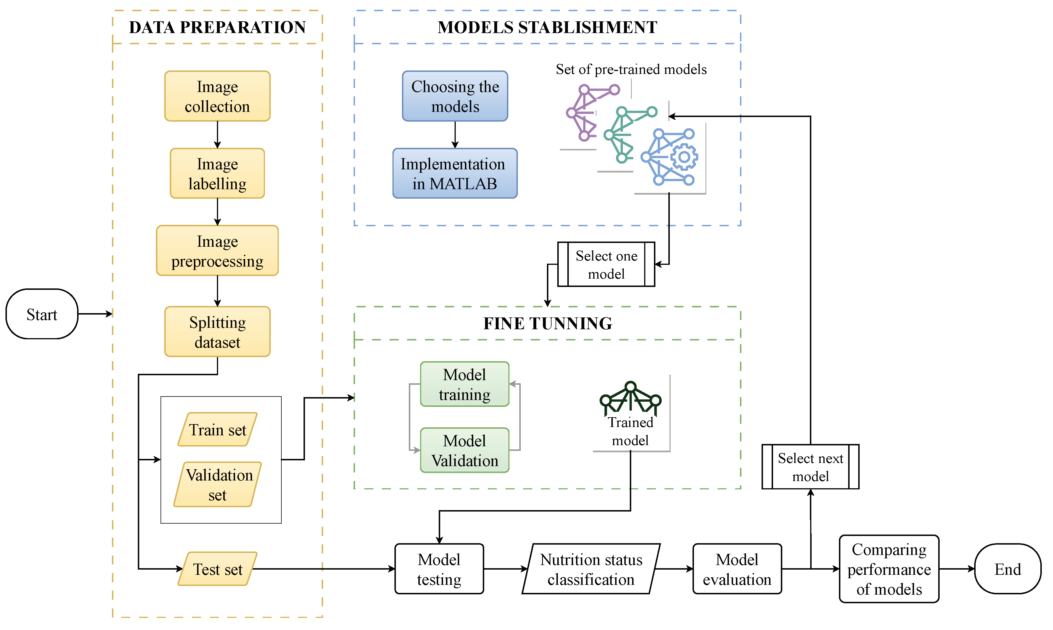
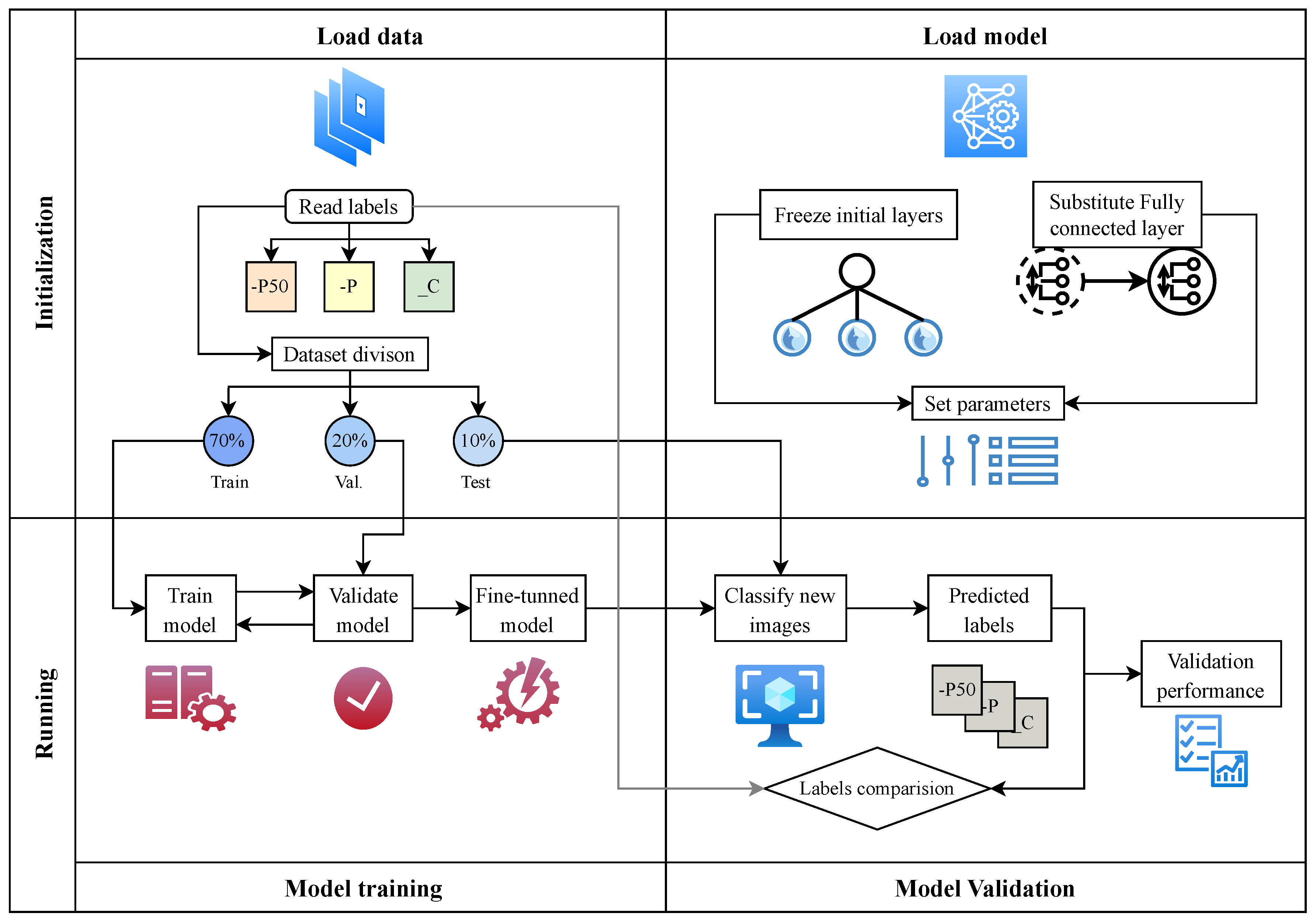
The workflow employed in this study, approaching the use of deep learning techniques to classify three levels of phosphorus deficiency in maize leaves, is illustrated in
Figure 1.
Firstly, a data preparation stage begins which involves the collection, labeling, preprocessing, and splitting of data. This stage ends with the labeled samples divided into three data sets: Train, validation, and test. In the second stage, a set of pre-trained models is chosen and implemented in MATLAB. One is selected for a fine-tuning stage, in which the inputs are the training and validation sets, and the output is a trained model. Hence, the fine-tuned model is used to classify new images from the test set. The prediction results are then evaluated with classification metrics, and the next model is chosen from the aforementioned set to restart the second stage. Once all pre-trained models have been tested, a comprehensive performance evaluation is conducted based on the metric scores, thereby concluding the workflow.
The following subsections will present the procedures’ details, providing a full overview of their specific information and methodologies.
2.1. Dataset building
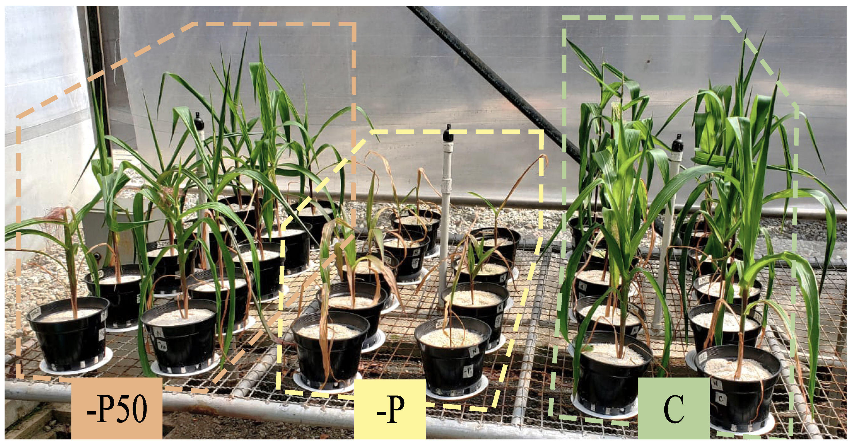
The images of nutrition-deficient maize leaves (
Zea mays L. improved variety ICA - V 109) used in this study were collected from mid-June to early August 2022 in a plastic shed from the area of Natural Systems and Sustainability of Universidad EAFIT, Medellin, Colombia (6°11’53.80" N, 75°34’43.23" W). The experimental design followed a
scheme, comprising ten replications on three phosphorus levels: P absence (-P), half dose (-P50), and complete supply (C), resulting in a total of 30 plants (See
Figure 2).
To induce the phosphorus deficiency levels, Hoagland’s complete solution [
4] was modified, taking into account only macronutrients and adjusting the net contribution of each nutrient according to the concentration of minerals in the solution.
2.1.1. Image collection
A total of 3934 images were acquired. Photographs included the growth stages of seedling, jointing, and flowering. The experiment involved natural illumination. Both sunny and cloudy days were considered to increase diversity in the illumination conditions.
Five acquisition devices were utilized, encompassing two types of regular smartphones, a digital camera, a single-lens reflex camera, and a compact scientific camera. In
Appendix A, the specifications of the tested cameras are presented. Nevertheless, previous experiments have determined that images captured by the scientific camera consistently yield superior classification performance. The outcomes of image classification using the GoogLeNet architecture for each camera type are provided in
Appendix B. Consequently, this study exclusively concentrates on the dataset comprising images acquired solely by the scientific camera. The specifications of this device are presented in
Table 1.
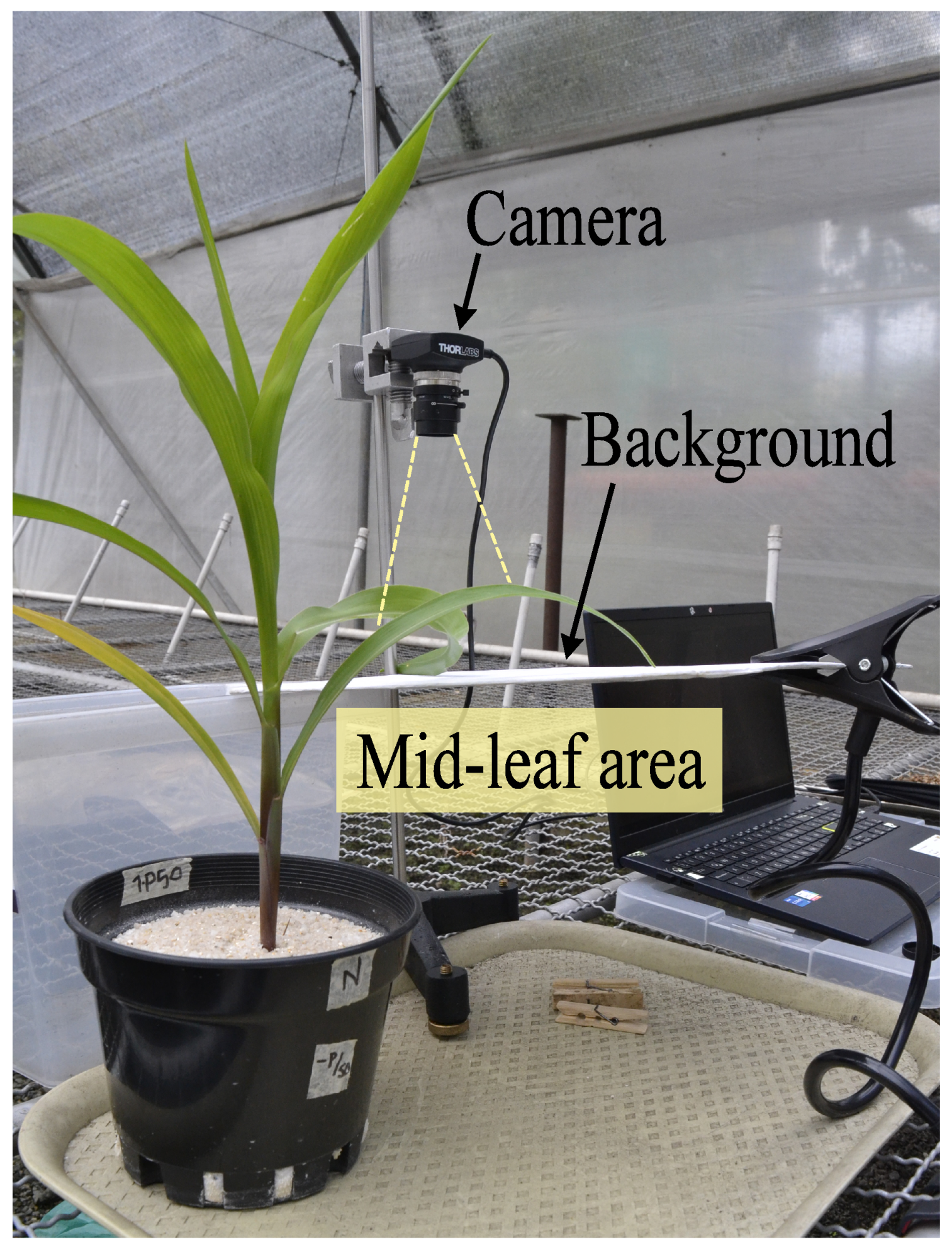
The image collection process was conducted according to the following steps: (1) One leave per plant exhibiting prominent visual symptoms, predominantly observed in older leaves, were selected for sampling. Specifically, the mid-leaf area, as depicted in
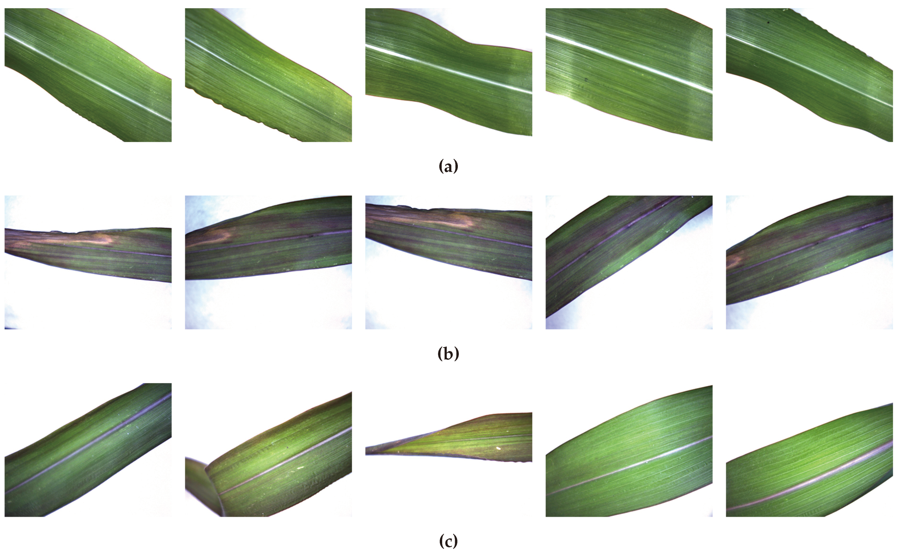
Figure 3, was the focal region of interest. (2) A white background sheet was carefully positioned trying to prevent the formation of shadows caused by the leaf and to minimize background-related noise. (3) The leaf was securely held, and a total of five photographs were captured for each leaf. Either the capture angle or the leaf section were adjusted between each shot, ensuring diverse perspectives. An illustration of this process is presented in
Figure 4.
The resulting images are saved and labeled according to the treatment and growth stage. Examples of images obtained using this method are shown in
Figure 4.
2.1.2. Image pre-processing and data augmentation
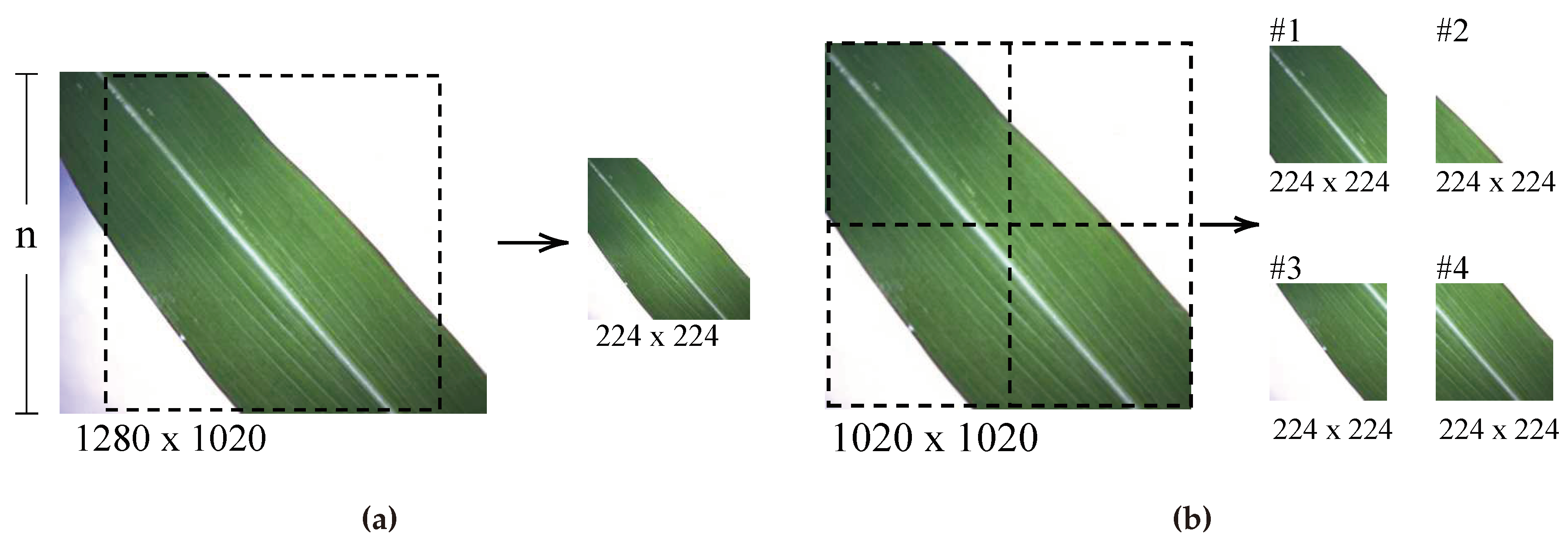
The original images obtained with the scientific camera underwent automatic size processing on Python code using two concurrent methods: (1) All
pixels size original images were cropped to a central square, with sides equal to the smallest image size (n), i.e. 1020 px. Then, cropped images were resized to
pixels size according to the method shown in
Figure 5a. (2) All images cropped to a central square were subsequently divided into four individual images with a size of
pixels each. Similarly, these cropped images were resized to
pixels. The process is shown in
Figure 5.
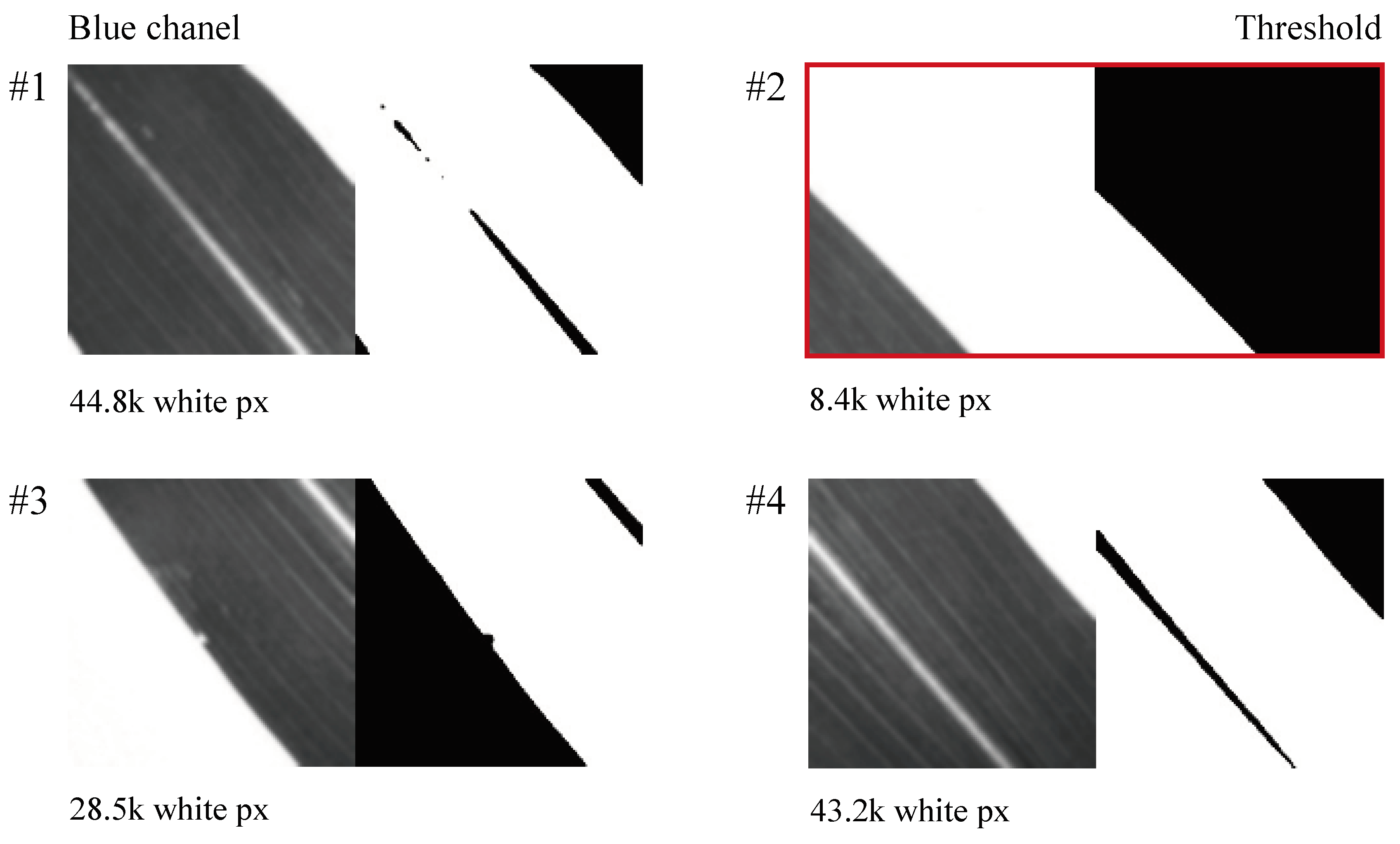
After the above process, the number of images increased fivefold. However, the automated cropping mechanism introduced certain issues, including producing blank images or images capturing only a small portion of the leaf which lead to images with limited or irrelevant content. An example of this is seen in image
of
Figure 5b. To address this problem, an algorithm was developed for selecting the valid images. The algorithm involved the following steps: first, the image was split into its RGB components. Based on the histogram analysis of the images, it was determined that the blue (B) channel provided more contrast to distinguish the leaf from the background, so that only the B channel was preserved. Next, a thresholding process was applied to distinguish leaf pixels (set to 255) from the background (set to 0). The algorithm then counted the number of leaf pixels, considering a minimum count of 15k pixels as indicative of a significant leaf presence. Finally, images with a pixel count below this threshold were excluded from further analysis. The effectiveness of the filtering process is illustrated in
Figure 6.
Following the preprocessing and data augmentation procedures, the resulting dataset contained the number of images indicated in
Table 2.
Finally, the training, validation, and testing image sets were composed with a ratio of 7:2:1, and the correspondence of the total of images is detailed in
Table 3.
2.2. Transfer Learning Approach
A deep learning approach is employed to classify the three levels of phosphorus deficiencies. Given the challenges associated with acquiring an ample supply of images and the potential scarcity of publicly available datasets for training convolutional neural networks (CNNs), it is common practice to adopt transfer learning. Transfer learning is a powerful machine learning technique that involves repurposing an existing trained model for a new problem, often related. This approach capitalizes on the capability of the initial layers in the original model to detect general features. Subsequently, the output of the last layer is adapted to the specific requirements of the new task. This adjustment is achieved by replacing the last fully-connected layer with a new one representing the classes relevant to the new problem. Additionally, it is possible to fine-tune the transfer learning process by selectively freezing or updating specific weights in the initial layers [
20].
The models used for transfer learning in this study are primarily associated with the ImageNet Large Scale Visual Recognition Challenge (ILSVRC) [
21], which has produced some of the most accurate models. These models have served as inspiration for numerous versions and improvements, as well as being the foundation for other models. Considering the existing literature, five architectures were selected based on their frequent utilization and high accuracy. Therefore, the following models were included in this study.
2.2.1. VGG16
These models were introduced in 2014 by Oxford’s Visual Geometry Group [
22] but are still popular today. The VGG networks consist of multiple blocks of stacked convolutional layers with smaller filters (i.e.
layers), combined with a max-pooling and another fully-connected layer. This set of layers is used instead of a larger filter size (such as
), which increases efficiency and makes the decision function more discriminative [
20]. The latter ultimately means that this model type generalizes well to a wide range of tasks [
22]. One of the most popular variants is VGG16, composed of 16 layers in weight and is available as a pre-trained model on the ImageNet dataset [
23].
2.2.2. ResNet50
Residual networks were first introduced in 2015 by He et al. [
24] and consist of blocks with two or three sequential convolutional layers with a parallel but separate identity layer that connects the input of the first layer and the output of the last one [
20]. These identity layers called skip connections solve errors generated at training and testing when the model goes deeper. Furthermore, they can mitigate the vanishing gradient problem when placed before the activation function [
25]. This study utilizes ResNet50, one of the evolved versions of ResNet. ResNet50 is chosen as it is a 50-layer deep architecture known for its remarkable performance and effectiveness in various tasks.
2.2.3. GoogLeNet
The GoogLeNet model is a special manifestation of the Inception architecture. This type of block splits the input into parallel and multiple pillars containing convolutional layers with a different-sized filter and a pooling layer. Those are followed or preceded by a downsampling convolution to reduce the output depth, which is finally concatenated. This enables saving computing resources [
20]. GoogLeNet structure uses nine Inception modules accompanied by pooling, regularization, and fully connected layers. For additional information, refer to the original paper [
26].
2.2.4. DenseNet201
Dense Convolutional Network (DenseNet) creators [
27] took some inspiration from the residual network’s idea to introduce dense blocks. These are modules of sequential convolutional layers, where any layer has a connection to every other layer in a feed-forward way in terms of concatenation operation. In this way, successive layers receive information from preceding ones, including feature maps, for better feature propagation and reuse. This process causes the number of channels to grow, despite reducing the number of parameters as compared to conventional CNN [
28]. Three versions are highlighted: DenseNet121, DenseNet169, and DenseNet201, which are differentiated by the number of layers. The latter is used in this study.
2.2.5. MobileNetV2
MovileNet was first introduced by Howard et al. [
29] using the concept of depthwise separable blocks, which consists of depthwise convolution, performing a single convolutional filter per input channel, followed by pointwise convolution, computing a linear
convolution of the input channels. Later, Sandler et al. [
30] improved the original version by incorporating bottleneck blocks between input and output layers, similar to residual connections, but considerably more memory efficient [
31].
2.3. Models Implementation
The transfer learning models are implemented using MATLAB’s Deep Learning Toolbox™ package (R2020a) [
32]. This package provides access to the pre-trained models mentioned earlier, which have been specifically trained on the ImageNet dataset. Some specifications of these models are presented in
Table 4.
The computer code is executed on a machine equipped with an i7-9700K 3.6 GHz processor, 64 GB RAM, and NVIDIA GeForce RTX 2080 40 GB GPU. To apply the transfer learning approach for each model, the following process is performed (see
Figure 7):
(1) Data with its ground-truth labels are read. These images are randomly chosen to form the train set with
of available samples,
for the validation set, and the remaining
images are used as a test set. (2) Each model is loaded separately and its initial layers are frozen to reuse the already learned general features. Moreover, the last fully-connected layer is substituted to match the three classes’ output in this study. (3) Hyperparameters are predefined with specific values as outlined in
Table 5. These hyperparameters control various aspects of the deep learning model and its training process. The details and explanations of these hyperparameters will be provided in the following paragraph. (4) The training process involves training each model on the train set and validating it at each epoch using the validation set. The training continues until either the maximum number of epochs requirement is met or the validation patience is satisfied. (5) The fine-tuned model is used to classify new images from the testing set. Consequently, the predicted labels are obtained. (6) The predicted labels are compared with the ground-truth labels to validate the model’s performance.
In
Table 5, the Solver represents the optimizer used for the loss function, which is stochastic gradient descent with a momentum of 0.9. The batch size indicates the number of images processed by the network in each batch for error computation and weight updates. The initial learning rate is used at the beginning of training and decreases by 0.96 per epoch in a stepwise manner. To prevent overfitting, the training process considers both a maximum number of epochs and a validation patience method. The validation patience method monitors the validation error for a consistent behavior within a certain number of epochs to determine when to stop training.
The hyperparameters presented in
Table 5 were determined based on findings reported in the existing literature for similar studies: Zhang et al. [
10], Mohanty et al. [
33], Barbedo [
34], Maeda-Gutiérrez et al. [
35] and Nagaoka [
36]. These values have been widely used and recognized as effective choices for achieving good performance in deep learning models.
3. Results
The proposed transfer learning approach was employed to classify three levels of phosphorus maize-leaf deficiency using the aforementioned deep learning models (VGG16, ResNet50, GoogLeNet, DenseNet201, and MobileNetV2). The following subsections describe the evolution of accuracy and loss values during the training stage and present the results obtained to evaluate the overall performance of the studied models on the dataset built specifically for this study.
3.1. Learning curves
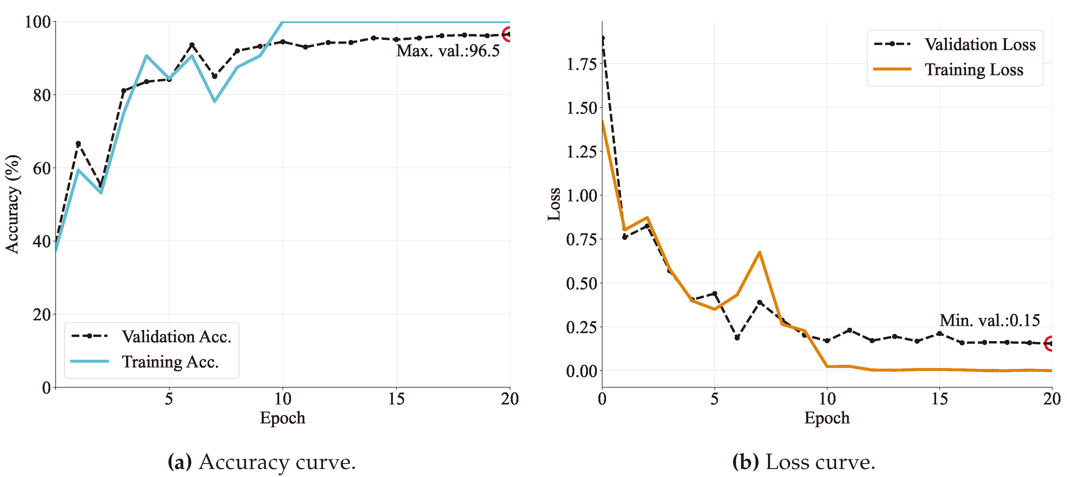
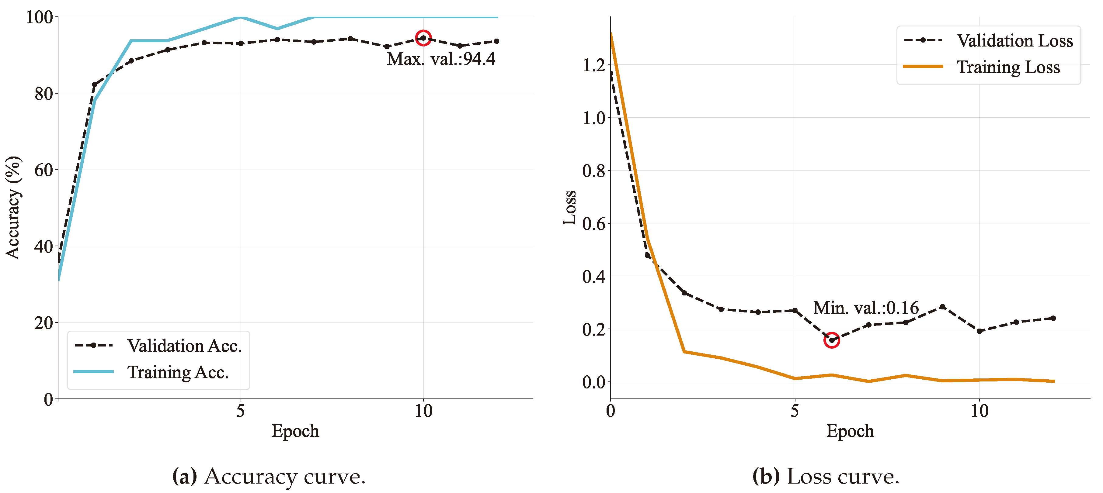
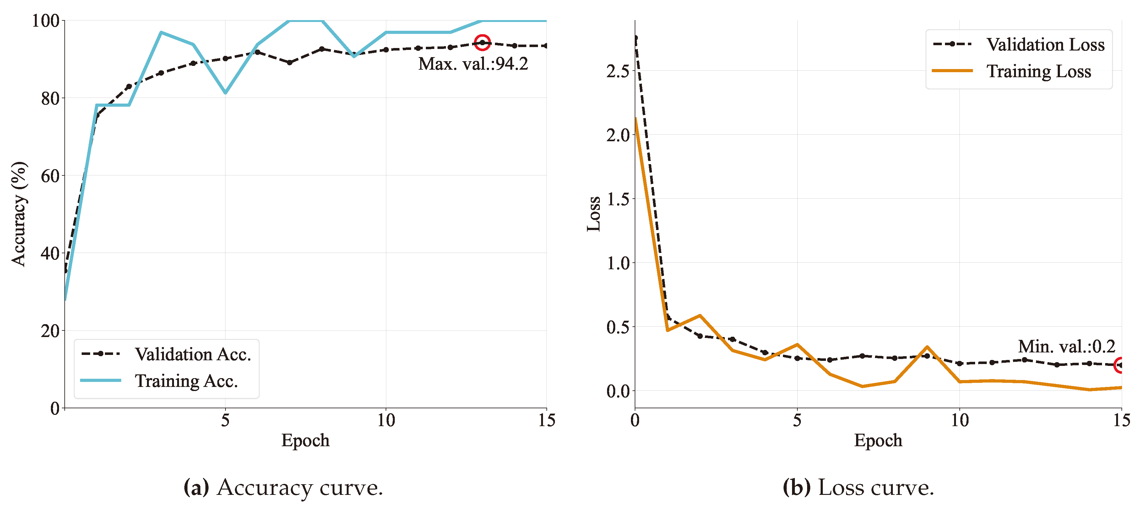
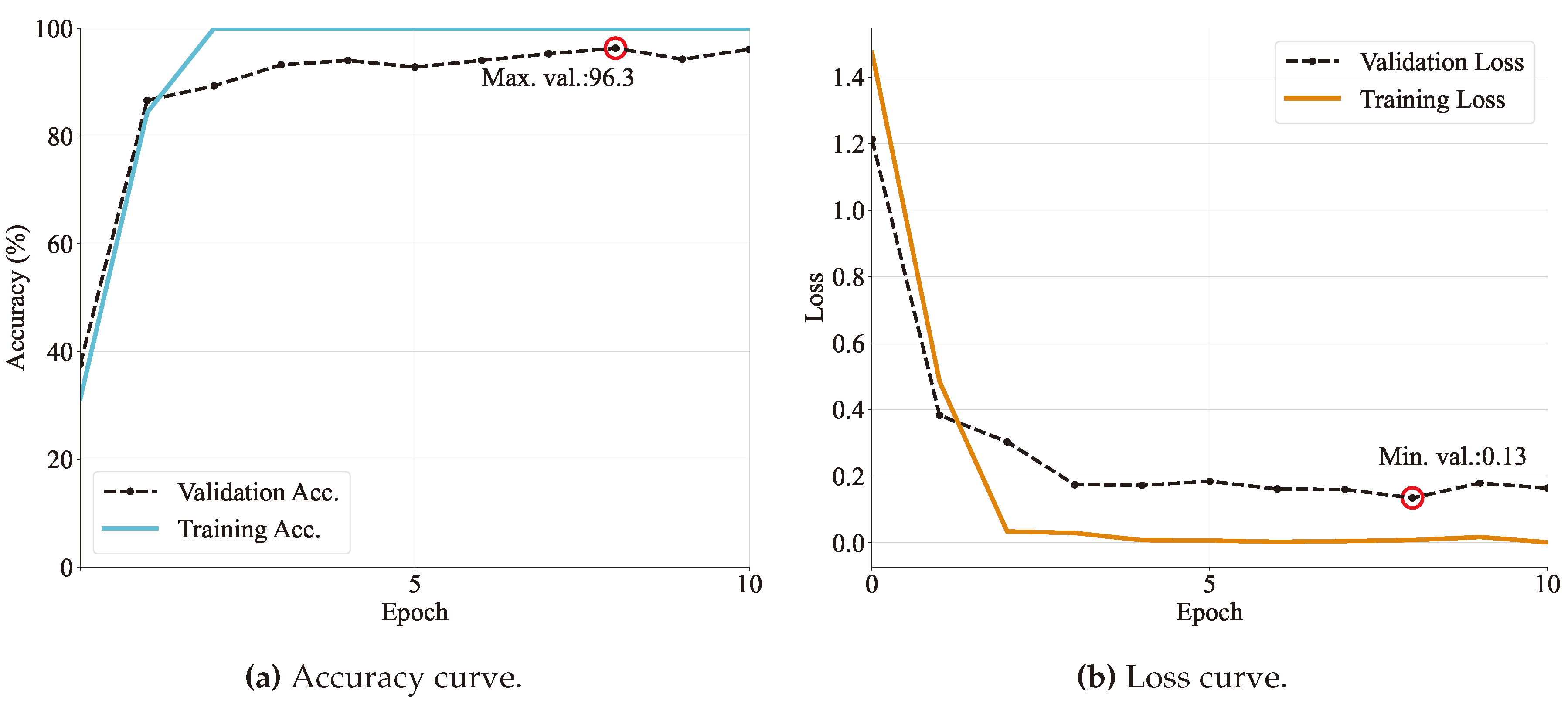
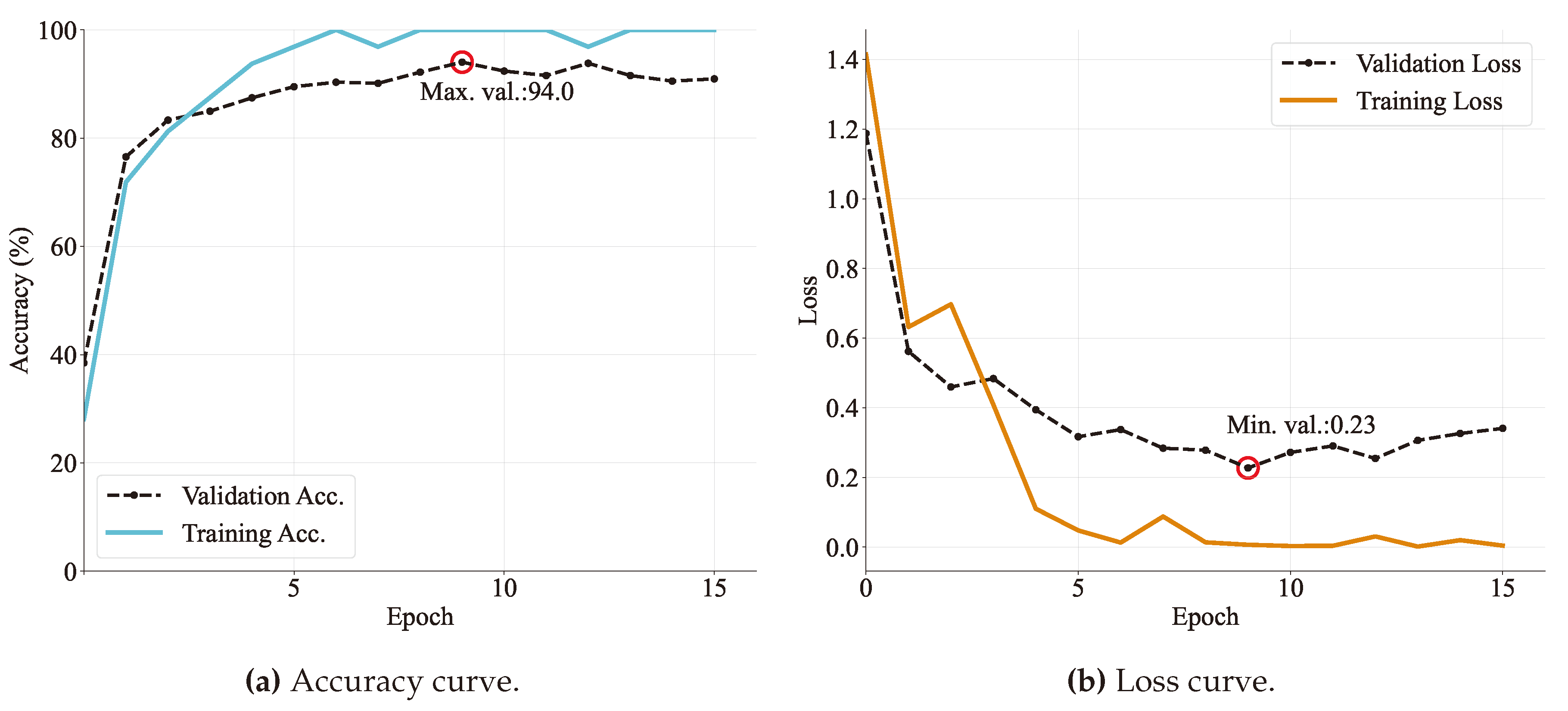
To evaluate the training performance, accuracy and loss curves are examined for each epoch.
Figure 8,
Figure 9,
Figure 10,
Figure 11 and
Figure 12 – depict the training progress with the train set, visually representing how well each model is learning. On the other hand, the validation curves in those figures provide insight into how well the model is generalizing.
Each model was run for 20 epochs and it was found that around five to ten epochs the models started to converge with high accuracy. Specifically, VGG and DenseNet models achieved more than in validation accuracy. Followed by MobileNet, ResNet, and GoogLeNet models that obtained an accuracy of more than on validation sets. In the same way, as is expected, losses seem to be lower as accuracy increases. Obtaining values ranging from 0.13 to 0.23.
In addition, model behavior can be diagnosed by the shape of the learning curves. One common dynamic that can be concluded by observing the graphs is overfitting. It refers to a model that has learned too closely the training dataset. This causes it to be less able generalizing unseen data. Based on
Figure 9 and
Figure 12 and Resnet and MobileNet loss validation curves continue to increase after a minimum validation point. That is the reason why the training is stopped at that moment, producing a training time of only 5 and 9 epochs, respectively.
Another consideration to be seen on learning curves is the gap between the validation and training loss curves, meaning an insufficient dataset size. It can be observed that both Resnet and MobileNet models have a more considerable gap distance, followed by GoogleNet and DeseNet (
Figure 10 and
Figure 11).
Finally, the most consistent performance is done by the VGG model in
Figure 8, since both curves reach a point of stability with a minimal gap between the final values. In addition, the training stops in the maximum number of epochs, indicating good learning and generalization of features in the images.
3.2. Performance analysis
Once each model is trained, it can further be used to infer features of interest in unknown data to test its generalization. In order to both assess the effectiveness of the studied models and to determine the superiority of one model over others, four performance metrics were utilized, as described below:
Accuracy: This is the most common classification metric. This metric describes the ratio between the number of correct predictions and the size of the data. The metric is defined in Equation
1.
Precision: This is a performance metric that measures the proportion of correct predictions for a specific class out of all the predictions made by the model for that class. It provides insights into the model’s ability to accurately classify instances for a particular class, regardless of the overall accuracy. Precision focuses on the relevance of the model’s predictions compared to the actual ground truth. This metric is defined in Equation
2.
Recall: Also known as sensitivity or true positive rate, is a performance metric that measures the proportion of correctly predicted instances for a specific class out of all the instances that actually belong to that class. It quantifies the model’s ability to identify and capture the positive instances, or true positives, in relation to the actual ground truth. Recall emphasizes the model’s capability to recognize and recall the relevant instances of a particular class, without considering the incorrect predictions. This metric is computed as presented in Equation
3.
F1-score: The F1-score is a performance metric that combines precision and recall into a single value by taking their harmonic mean. By incorporating both precision and recall, the F1-score provides a comprehensive evaluation of the model’s ability to achieve both high precision and high recall, promoting a balanced trade-off between the two measures. The metric is defined by Equation
4.
Since the metrics of precision, recall, and F1-score are performance measures for
n classes, there are different ways to combine these scores to have an overall value. One way to do this is to calculate the simple arithmetic mean, which is known as the macro-averaged score as defined by Equation
5. With this technique, all classes contribute equally to the final averaged metric.
Table 6 presents a comparison of the performance metrics, including macro-averaged precision, recall, F1-score, and accuracy, on the testing set. It is highlited the model with the best result, corresponding to VGG16.
In these terms, MobileNet obtained the lowest scores followed by GoogLeNet and ResNet architectures. As was discussed observing the learning curves, those models had problems with training, in terms of overfitting and insufficient dataset size. Both aspects would impact negatively the model’s performance. In the same way, the more consistent training was done by DenseNet and VGG and this is depicted on its high performance.
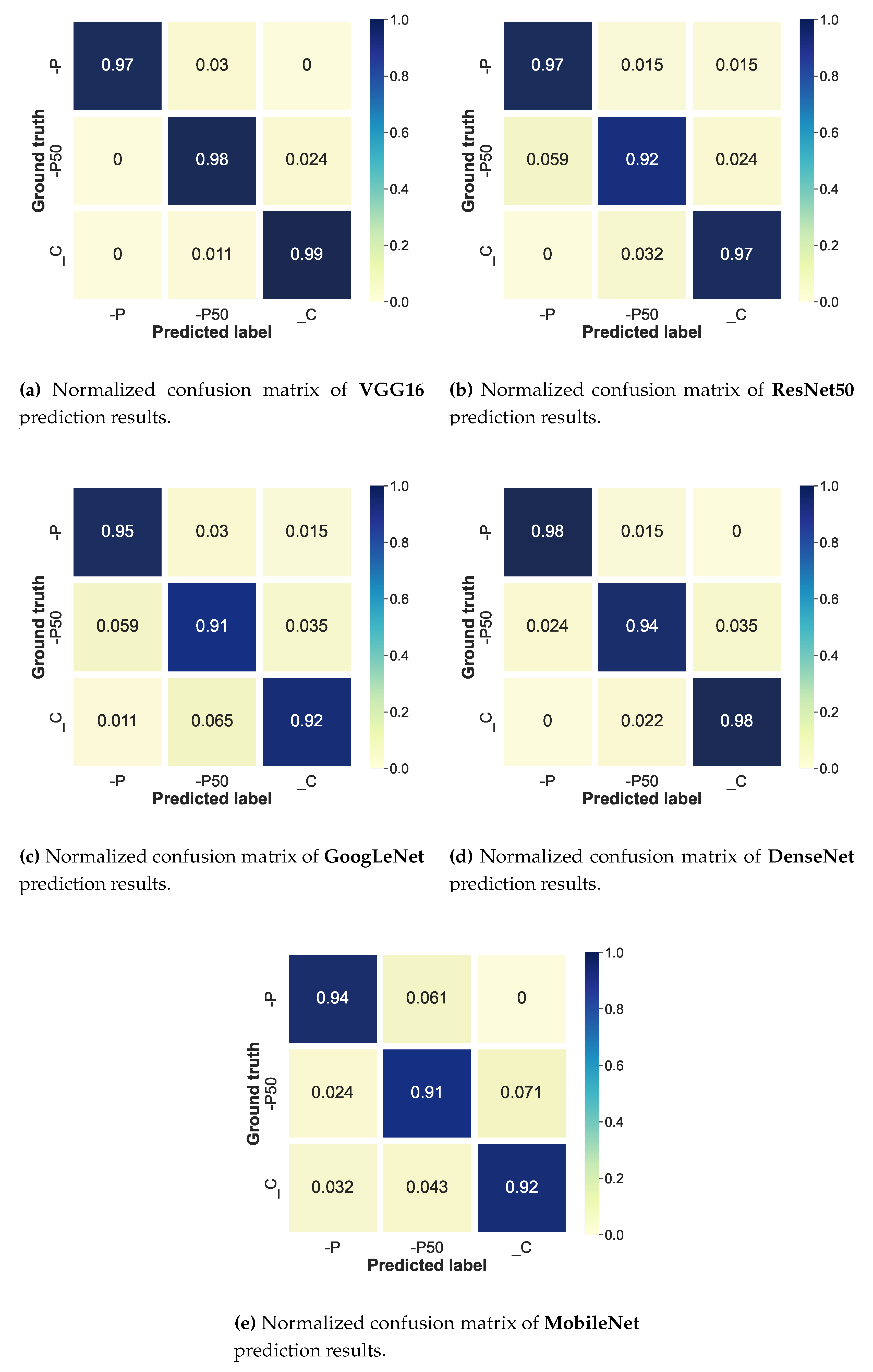
To finish the evaluation of the studied models, the confusion matrix is used. This tool records all the predictions made on the test set, allowing the visualization of the performance for each class. On one side of the matrix, the ground truth is arranged against predictions of the model. The confusion matrices for all models are shown in
Figure 13.
Based on the graphics, it can be seen that in almost all cases the prediction of
class has the lowest performance values, except on the VGG model (
Figure 13a) which has lower recognition rates for
label. Concerning this architecture, the color map allows noticing a high homogeneity of correct classifications for all classes, i.e., this model has no strong inclination to recognize one class more than another. In the opposite case, it can be seen in
Figure 13b that the ResNet model has a classification weakness on the
label (
accuracy), although all other classes are identified with high accuracy (both with
). This same behavior is traced by DenseNet in
Figure 13d but with a slightly higher accuracy rate. Finally, the most heterogeneous distribution in recognition is given by the architectures of GoogLeNet and MobileNet (on
Figure 13c and
Figure 13e, respectively).
This difficulty in recognizing the label is observed in almost all models and is explained by the overlap of visual characteristics between this class and the other two. This makes it as difficult for a human as it is for a machine to recognize the differences between a leaf with sufficient nutrition or low nutrition and a leaf with medium nutrition.
Despite nutrition evaluation is relevant to ensure good agricultural production, other issues such as maize diseases develop the same deep learning framework, so it is possible to compare results obtained by other studies from the literature, which are presented in
Table 7. It was observed from the analysis that this work is placed within the state-of-the-art results, and also that only a few studies attempt to acquire own images.
4. Conclusions
The detection and identification of plant-leaf issues is a relevant task in farm management. The care of each plant leads to a healthy plantation, which will result in high production of excellent quality. Regardless there are many developed deep learning methods for the classification of plant diseases, including leaf nutrition deficiency, they do not respond the same to all situations. That’s why the behavior analysis of these deep learning models for specific tasks is crucial in the development of automated systems to support agricultural activities. In this study, five transfer deep learning architectures pre-trained on the ImageNet database (i.e. VGG16, ResNet50, GoogLeNet, DenseNet201, and MobileNetV2) were trained to classify three phosphorus deficiency levels on a self-made database, whose images were taken by five different acquisition devices but just one camera images were selected for this analysis. It was found that VGG16 performed the best for this specific problem, giving the most consistent training performance and best recognition metrics, leading an overall accuracy score of , as well as correct-prediction rates equally distributed along all classes. No such remarkable results for the VGG model was found in previous studies, so further investigations can be done focusing on the performance of this architecture against more current models. The second best-behaved model was DenseNet201 reaching an accuracy of , but with better recognition rates for and C labels than for those with . Finally, GoogLeNet and MobileNet had the lower overall accuracy ( and respectively). The first, probably by its huge number of layers, it’s either not learning enough features from the database, or more data is required to correctly adjust the network weights. The same issue is possibly happening with the second model, judging by the shape of the loss curve which also indicates some overfitting. Moreover, the analysis of learning curves supports this hypothesis and allows to understand that for most architectures, the amount of training data is not sufficient for the models to make a perfect generalization of the features in the images. Therefore, it is necessary to increase the size of the database in the future. In the same way, different regularization techniques can be explored to avoid overfitting. This study contributes to a faster and economical identification of nutritional phosphorus issues, so that the crop’s fertilization schedule can focus efforts on specific plants, and thus make a more rational use of resources, taking care of both the farmer’s budget, as well as the health of the environment. We remark that the setup proposed in this research can be extended easily to real-time monitoring of other crops types, even to analyze different kinds of leaf-issues that could be inferred from visual inspection.
Author Contributions
Conceptualization, M.R. and A.M.; methodology, investigation, formal analysis, software and visualization, M.R.; validation, M.R., A.M., L.G. and C.T.; resources, A.M. and C.T.; Project administration, supervision and funding acquisition, A.M.; writing – original draft, M.R.; writing – review & editing, A.M., C.T. and L.G. All authors have read and agreed to the published version of the manuscript.
Funding
This research was funded by Universidad EAFIT.
Data Availability Statement
Acknowledgments
M. Ramos-Ospina and A. Marulanda-Tobón acknowledge the support from María Isabel Hernández-Pérez, head of the Undergraduate Program in Agricultural Engineering, from School of Applied Sciences and Engineering, Universidad EAFIT, for the scientific assistance provided during the realization of this work.
Conflicts of Interest
The authors declare no conflict of interest.
Appendix A. Original image acquisition devices
Table A1.
Specifications of cameras used to acquire original images.
Table A1.
Specifications of cameras used to acquire original images.
| Camera type |
Smartphone 1: Xiaomi Redmi 8T |
Smartphone 2: Moto G (5) Plus |
Digital |
Single-lens reflex |
Compact Scientific |
| Manufacturer |
Omnivision |
Motorols |
Samsung |
Nikon |
ThorLabs |
|
Model |
OV02A10 |
Unknown |
ES65 |
D3100 |
DCC1645C-HQ |
|
Sensor type |
CMOS |
Unknown |
CCD |
CMOS |
Color CMOS |
| Number of Active Pixels |
|
|
|
|
|
| Resolution (ppp) |
96 |
72 |
96 |
300 |
144 |
| Optical Format |
0.2" |
0.4" |
0.24" |
1.09" |
0.33" |
| Maximum aperture f / |
2.4 |
1.7 |
3.5 |
3.8 |
1.4 |
Appendix B. Previous results on different camera types
Table A2.
Results on classification of images using GoogLeNet architecture according to camera type.
Table A2.
Results on classification of images using GoogLeNet architecture according to camera type.
| Metric |
Accuracy |
Average precision |
Average recall |
| Smartphone 1 |
0.84 |
0.84 |
0.84 |
|
Smartphone 2 |
0.91 |
0.92 |
0.92 |
|
Digital |
0.80 |
0.81 |
0.80 |
|
Reflex |
0.92 |
0.92 |
0.92 |
|
Scientific |
0.93 |
0.92 |
0.93 |
References
- Salmerón, J.I.C. Historia General de la Agricultura, 1 ed.; Vol. 1, Guadalmazán, 2018; pp. 1–840.
- Tian, H.; Wang, T.; Liu, Y.; Qiao, X.; Li, Y. Computer vision technology in agricultural automation —A review. Information Processing in Agriculture 2020, 7, 1–19. [Google Scholar] [CrossRef]
- Leena, N.; Saju, K.K. Classification of macronutrient deficiencies in maize plants using optimized multi class support vector machines. Engineering in Agriculture, Environment and Food 2019, 12, 126–139. [Google Scholar] [CrossRef]
- Taiz, L.; Zeiger, E. Plant physiology, 4 ed.; Vol. 1, Sunderland, Mass, 2006; pp. 0–764.
- White, P.J.; Hammond, J.P. The Ecophysiology of Plant-Phosphorus Interactions; Vol. 7, Springer Netherlands, 2008; p. 296. [CrossRef]
- Condori, R.H.M.; Romualdo, L.M.; Bruno, O.M.; Luz, P.H.D.C. Comparison between Traditional Texture Methods and Deep Learning Descriptors for Detection of Nitrogen Deficiency in Maize Crops. Proceedings - 13th Workshop of Computer Vision, WVC 2017 2018, 2018-Janua, 7–12. [CrossRef]
- Smith, M.L.; Smith, L.N.; Hansen, M.F. The quiet revolution in machine vision - a state-of-the-art survey paper, including historical review, perspectives, and future directions. Computers in Industry 2021, 130, 103472. [Google Scholar] [CrossRef]
- Barbedo, J.G.A. Detection of nutrition deficiencies in plants using proximal images and machine learning: A review. Computers and Electronics in Agriculture 2019, 162, 482–492. [Google Scholar] [CrossRef]
- Barbedo, J.G. Factors influencing the use of deep learning for plant disease recognition. Biosystems Engineering 2018, 172, 84–91. [Google Scholar] [CrossRef]
- Zhang, X.; Qiao, Y.; Meng, F.; Fan, C.; Zhang, M. Identification of maize leaf diseases using improved deep convolutional neural networks. IEEE Access 2018, 6, 30370–30377. [Google Scholar] [CrossRef]
- Hughes, D.P.; Salathe, M. An open access repository of images on plant health to enable the development of mobile disease diagnostics. arXiv e-prints 2015.
- Bhatt, P.; Sarangi, S.; Shivhare, A.; Singh, D.; Pappula, S. Identification of Diseases in Corn Leaves using Convolutional Neural Networks and Boosting. 2019, pp. 894–899. [CrossRef]
- Chen, J.; Chen, J.; Zhang, D.; Sun, Y.; Nanehkaran, Y.A. Using deep transfer learning for image-based plant disease identification. Computers and Electronics in Agriculture 2020, 173, 105393. [Google Scholar] [CrossRef]
- Zeng, W.; Li, H.; Hu, G.; Liang, D. Identification of maize leaf diseases by using the SKPSNet-50 convolutional neural network model. Sustainable Computing: Informatics and Systems 2022, p. 100695. [CrossRef]
- Verma, A.; Bhowmik, B. Automated Detection of Maize Leaf Diseases in Agricultural Cyber-Physical Systems. Institute of Electrical and Electronics Engineers Inc., 2022, pp. 841–846. [CrossRef]
- Zúñiga, A.M.G.; Bruno, O.M. Sistema de visão artificial para identificação do estado nutricional de plantas. Master’s thesis, Sciences of computation and mathematical computation, 2012.
- de Fátima da Silva, F.; Luz, P.H.C.; Romualdo, L.M.; Marin, M.A.; Zúñiga, A.M.G.; Herling, V.R.; Bruno, O.M. A Diagnostic Tool for Magnesium Nutrition in Maize Based on Image Analysis of Different Leaf Sections. Crop Science 2014, 54, 738–745. [Google Scholar] [CrossRef]
- Thorlabs Scientific Imaging,. DCx Camera Functional Description and SDK Manual. DCC1545M Specifications, 2018.
- Thorlabs Scientific Imaging,. Camera Lenses for Machine Vision | MVL6WA.
- Vasilev, I.; Slater, D.; Spacagna, G.; Roelants, P.; Zocca, V. Python deep learning: exploring deep learning techniques and neural network architectures with PyTorch, Keras, and TensorFlow, 2 ed.; Vol. 1, Packt Publishing, 2019; p. 379.
- Russakovsky, O.; Deng, J.; Su, H.; Krause, J.; Satheesh, S.; Ma, S.; Huang, Z.; Karpathy, A.; Khosla, A.; Bernstein, M.; Berg, A.C.; Fei-Fei, L.; Russakovsky, O.; Deng, J.; Su, H.; Krause, J.; Satheesh, S.; Ma, S.; Huang, Z.; Karpathy, A.; Khosla, A.; Bernstein, M.; Berg, A.C.; Fei-Fei, L. ImageNet Large Scale Visual Recognition Challenge. International Journal of Computer Vision 2014, 115, 211–252. [Google Scholar] [CrossRef]
- Simonyan, K.; Zisserman, A. Very Deep Convolutional Networks for Large-Scale Image Recognition. 3rd International Conference on Learning Representations, ICLR 2015 - Conference Track Proceedings 2014.
- Deng, J.; Dong, W.; Socher, R.; Li, L.J.; Li, K.; Fei-Fei, L. ImageNet: A large-scale hierarchical image database. Institute of Electrical and Electronics Engineers (IEEE), 2010, pp. 248–255. [CrossRef]
- He, K.; Zhang, X.; Ren, S.; Sun, J. Deep Residual Learning for Image Recognition. Proceedings of the IEEE Computer Society Conference on Computer Vision and Pattern Recognition 2015, 2016-December, 770–778. [CrossRef]
- Andrew, J.; Eunice, J.; Popescu, D.E.; Chowdary, M.K.; Hemanth, J. Deep Learning-Based Leaf Disease Detection in Crops Using Images for Agricultural Applications. Agronomy 2022, Vol. 12, Page 2395 2022, 12, 2395. [Google Scholar] [CrossRef]
- Szegedy, C.; Liu, W.; Jia, Y.; Sermanet, P.; Reed, S.; Anguelov, D.; Erhan, D.; Vanhoucke, V.; Rabinovich, A. Going Deeper with Convolutions. IEEE, 2015, pp. 1–9.
- Huang, G.; Liu, Z.; Maaten, L.V.D.; Weinberger, K.Q. Densely Connected Convolutional Networks. Proceedings - 30th IEEE Conference on Computer Vision and Pattern Recognition, CVPR 2017 2016, 2017-January, 2261–2269. [CrossRef]
- Pradhan, P.; Kumar, B.; Mohan, S. Comparison of various deep convolutional neural network models to discriminate apple leaf diseases using transfer learning. Journal of Plant Diseases and Protection 2022, 129, 1461–1473. [Google Scholar] [CrossRef]
- Howard, A.G.; Zhu, M.; Chen, B.; Kalenichenko, D.; Wang, W.; Weyand, T.; Andreetto, M.; Adam, H. MobileNets: Efficient Convolutional Neural Networks for Mobile Vision Applications. arXiv 2017. [Google Scholar]
- Sandler, M.; Howard, A.; Zhu, M.; Zhmoginov, A.; Chen, L.C. MobileNetV2: Inverted Residuals and Linear Bottlenecks. Proceedings of the IEEE Computer Society Conference on Computer Vision and Pattern Recognition 2018, pp. 4510–4520. [CrossRef]
- Hassan, S.M.; Maji, A.K.; Jasiński, M.; Leonowicz, Z.; Jasińska, E. Identification of Plant-Leaf Diseases Using CNN and Transfer-Learning Approach. Electronics 2021, Vol. 10, Page 1388 2021, 10, 1388. [Google Scholar] [CrossRef]
- Inc, T.M. Deep Learning Toolbox, 2020.
- Mohanty, S.P.; Hughes, D.P.; Salathé, M. Using deep learning for image-based plant disease detection. Frontiers in Plant Science 2016, 7, 1419. [Google Scholar] [CrossRef] [PubMed]
- Barbedo, J.G.A. Impact of dataset size and variety on the effectiveness of deep learning and transfer learning for plant disease classification. Computers and Electronics in Agriculture 2018, 153, 46–53. [Google Scholar] [CrossRef]
- Maeda-Gutiérrez, V.; Galván-Tejada, C.E.; Zanella-Calzada, L.A.; Celaya-Padilla, J.M.; Galván-Tejada, J.I.; Gamboa-Rosales, H.; Luna-García, H.; Magallanes-Quintanar, R.; Méndez, C.A.G.; Olvera-Olvera, C.A. Comparison of Convolutional Neural Network Architectures for Classification of Tomato Plant Diseases. Applied Sciences 2020, 10, 1245. [Google Scholar] [CrossRef]
- Nagaoka, T. Hyperparameter Optimization for Deep Learning-based Automatic Melanoma Diagnosis System. Advanced Biomedical Engineering 2020, 9, 225–232. [Google Scholar] [CrossRef]
Figure 1.
Workflow for phosphorous deficiency detection.
Figure 1.
Workflow for phosphorous deficiency detection.
Figure 2.
Location of experiments and treatments differentiation.
Figure 2.
Location of experiments and treatments differentiation.
Figure 3.
Illustration of an image acquisition example. The camera, the background sheet, and the leaf capture area are depicted.
Figure 3.
Illustration of an image acquisition example. The camera, the background sheet, and the leaf capture area are depicted.
Figure 4.
Example of five consecutive images taken from leaves with: (a) complete nutrition (C), (b) no phosphorus nutrition (-P), and (c) half-phosphorus nutrition (-P50).
Figure 4.
Example of five consecutive images taken from leaves with: (a) complete nutrition (C), (b) no phosphorus nutrition (-P), and (c) half-phosphorus nutrition (-P50).
Figure 5.
Pre-processing based on cropping and resizing images using two methods, named: (a) cut to square and (b) quadrant division.
Figure 5.
Pre-processing based on cropping and resizing images using two methods, named: (a) cut to square and (b) quadrant division.
Figure 6.
Selection process for images obtained through quadrant crop division. Each image shows the separated blue channel (left) and the result of thresholding (right). The number of white pixels at the bottom of each image represents the leaf content. A minimum count of 15k white pixels is considered as the threshold for determining the presence of relevant information. In this example, only image would be filtered out.
Figure 7.
Framework of transfer learning approach for each model.
Figure 7.
Framework of transfer learning approach for each model.
Figure 8.
Training and validation curves for the VGG16 architecture specifying (a) accuracy and (b) loss in every epoch. The maximum accuracy value and the minimum loss are also reported.
Figure 8.
Training and validation curves for the VGG16 architecture specifying (a) accuracy and (b) loss in every epoch. The maximum accuracy value and the minimum loss are also reported.
Figure 9.
Training and validation curves for the ResNet50 architecture specifying (a) accuracy and (b) loss in every epoch. The maximum accuracy value and the minimum loss are also reported.
Figure 9.
Training and validation curves for the ResNet50 architecture specifying (a) accuracy and (b) loss in every epoch. The maximum accuracy value and the minimum loss are also reported.
Figure 10.
Training and validation curves for the GoogLeNet architecture specifying (a) accuracy and (b) loss in every epoch. The maximum accuracy value and the minimum loss are also reported.
Figure 10.
Training and validation curves for the GoogLeNet architecture specifying (a) accuracy and (b) loss in every epoch. The maximum accuracy value and the minimum loss are also reported.
Figure 11.
Training and validation curves for the DenseNet201 architecture specifying (a) accuracy and (b) loss in every epoch. The maximum accuracy value and the minimum loss are also reported.
Figure 11.
Training and validation curves for the DenseNet201 architecture specifying (a) accuracy and (b) loss in every epoch. The maximum accuracy value and the minimum loss are also reported.
Figure 12.
Training and validation curves for the MobileNetV2 architecture specifying (a) accuracy and (b) loss in every epoch. The maximum accuracy value and the minimum loss are also reported.
Figure 12.
Training and validation curves for the MobileNetV2 architecture specifying (a) accuracy and (b) loss in every epoch. The maximum accuracy value and the minimum loss are also reported.
Figure 13.
Confusion matrices to evaluate the accuracy of prediction results for each model.
Figure 13.
Confusion matrices to evaluate the accuracy of prediction results for each model.
Table 1.
Compact scientific camera specifications [
18,
19].
Table 1.
Compact scientific camera specifications [
18,
19].
| Specification |
Value |
| Manufacturer |
ThorLabs |
|
Sensor Model |
DCC1645C-HQ |
|
Sensor type |
Color CMOS |
|
Resolution |
pixels (1.31 Megapixel) |
|
Optical Format |
1/3" |
|
Read noise |
<25 e- RMS |
|
Bit depth |
10 |
|
Lens Model |
MVL6WA |
|
Focal Length |
6 mm |
|
Maximum aperture |
f/1.4 |
Table 2.
Dataset details.
Table 2.
Dataset details.
| Class |
Description |
Number of images |
| -P |
No phosphorus nutrition |
656 |
| -P50 |
Half of phosphorus than complete nutrition |
850 |
| C |
Complete nutrition |
927 |
Table 3.
Dataset division.
Table 3.
Dataset division.
| Image set |
Number of samples |
| Total |
2433 |
| Train () |
1703 |
| Validation () |
487 |
| Test () |
243 |
Table 4.
Parameters of pre-trained CNN models.
Table 4.
Parameters of pre-trained CNN models.
| Model |
Depth (layers) |
Total parameters (in millions) |
Size (MB) |
Birth year |
| VGG16 |
16 |
138.0 |
515 |
2014 |
| ResNet50 |
50 |
25.6 |
96 |
2015 |
| GoogLeNet |
22 |
7.0 |
27 |
2014 |
| DenseNet201 |
201 |
20.0 |
77 |
2017 |
| MobileNetV2 |
53 |
3.5 |
13 |
2018 |
Table 5.
Hyperparameters specifications.
Table 5.
Hyperparameters specifications.
| Solver |
SGDM |
| Momentum |
0.9 |
| Batch size |
32 |
| Initial learning rate |
0.001 |
| Learning rate policy |
Step |
| Learning rate decay |
0.96 |
| Decay period |
1 epoch |
| Max epochs |
20 |
| Validation patience |
6 |
Table 6.
Comparative performance analysis on validation macro-averaged metrics for each model.
Table 6.
Comparative performance analysis on validation macro-averaged metrics for each model.
| Network model |
Accuracy |
Precision |
Recall |
F1-Score |
| DenseNet201 |
96.7 |
96.7 |
96.8 |
96.8 |
| MobileNet |
92.2 |
92.2 |
92.3 |
92.3 |
| ResNet50 |
95.1 |
94.9 |
95.2 |
95.0 |
| GoogleNet |
92.6 |
92.5 |
92.8 |
92.6 |
| VGG16 |
98.0 |
98.1 |
97.8 |
98.0 |
Table 7.
Comparison with literature-review results.
Table 7.
Comparison with literature-review results.
| Reference |
Dataset |
Multi-classes |
Pre-trained Model |
Metric |
Value |
| [13] |
PlantVillage |
4 |
VGG19 |
Training accuracy |
74.20 |
| ResNet50 |
70.41 |
| DenseNet201 |
84.13 |
| Porpoused "INC-VGGN" |
97.57 |
|
[15] |
Self-created |
4 |
VGG16 |
Test Accuracy |
97.35 |
| ResNet50 |
99.21 |
| DenseNet169 |
99.51 |
| Porpoused "MDCNN” |
99.54 |
|
[14] |
Self-created |
6 |
VGG16 |
Average F1-Score |
81.4 |
| ResNet50 |
82.5 |
| Porpoused "SKPSNet-50" |
91.9 |
|
[10] |
Various sources |
9 |
Improved GoogLeNet |
Test accuracy |
98.8 |
| Improved Cifar10 |
97.1 |
|
Disclaimer/Publisher’s Note: The statements, opinions and data contained in all publications are solely those of the individual author(s) and contributor(s) and not of MDPI and/or the editor(s). MDPI and/or the editor(s) disclaim responsibility for any injury to people or property resulting from any ideas, methods, instructions or products referred to in the content. |
© 2023 by the authors. Licensee MDPI, Basel, Switzerland. This article is an open access article distributed under the terms and conditions of the Creative Commons Attribution (CC BY) license (http://creativecommons.org/licenses/by/4.0/).
