1. Introduction
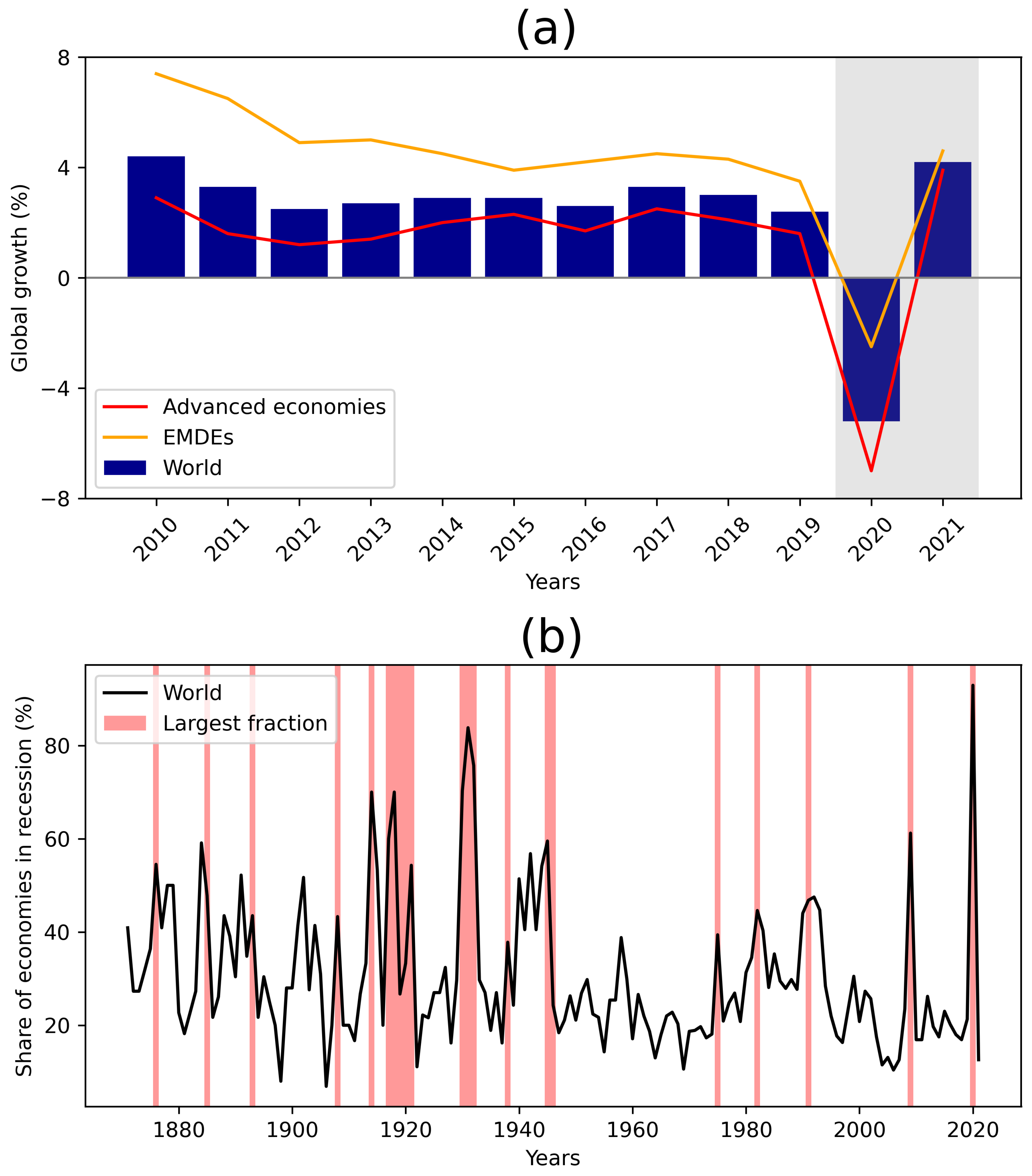
The COVID-19 pandemic, which originated in the city of Wuhan in late 2019, has resulted in the most significant global economic downturn since World War II (a 5% decline in global economic activity by 2020, according to the World Bank, June 2020). This crisis has had a profound impact on advanced economies, witnessing a 7% decline in 2020 (refer to
Figure 1a). Additionally, emerging economies experienced their first output contraction in at least 60 years, with a decline of -2.5% (Global Economic Prospect, World Bank, June 2020, see
Figure 1b).
In this context, the International Monetary Fund (IMF) has urged governments to consider implementing economic measures that can provide support to the population and productive sectors. The goal is to alleviate the significant economic losses and social hardships resulting from the pandemic. In response, the IMF has devised several initiatives. These include emergency financing options like the Rapid Credit Facility (RCF) and the Rapid Financing Instrument (RFI), which are specifically designed to address the financial requirements arising from health catastrophes. Additionally, the IMF has established the Catastrophe Relief and Containment Trust Fund, which facilitates assistance to underprivileged and vulnerable countries through donations, with a focus on managing public health crises effectively.
The specific case of Chile, as indicated by data from [
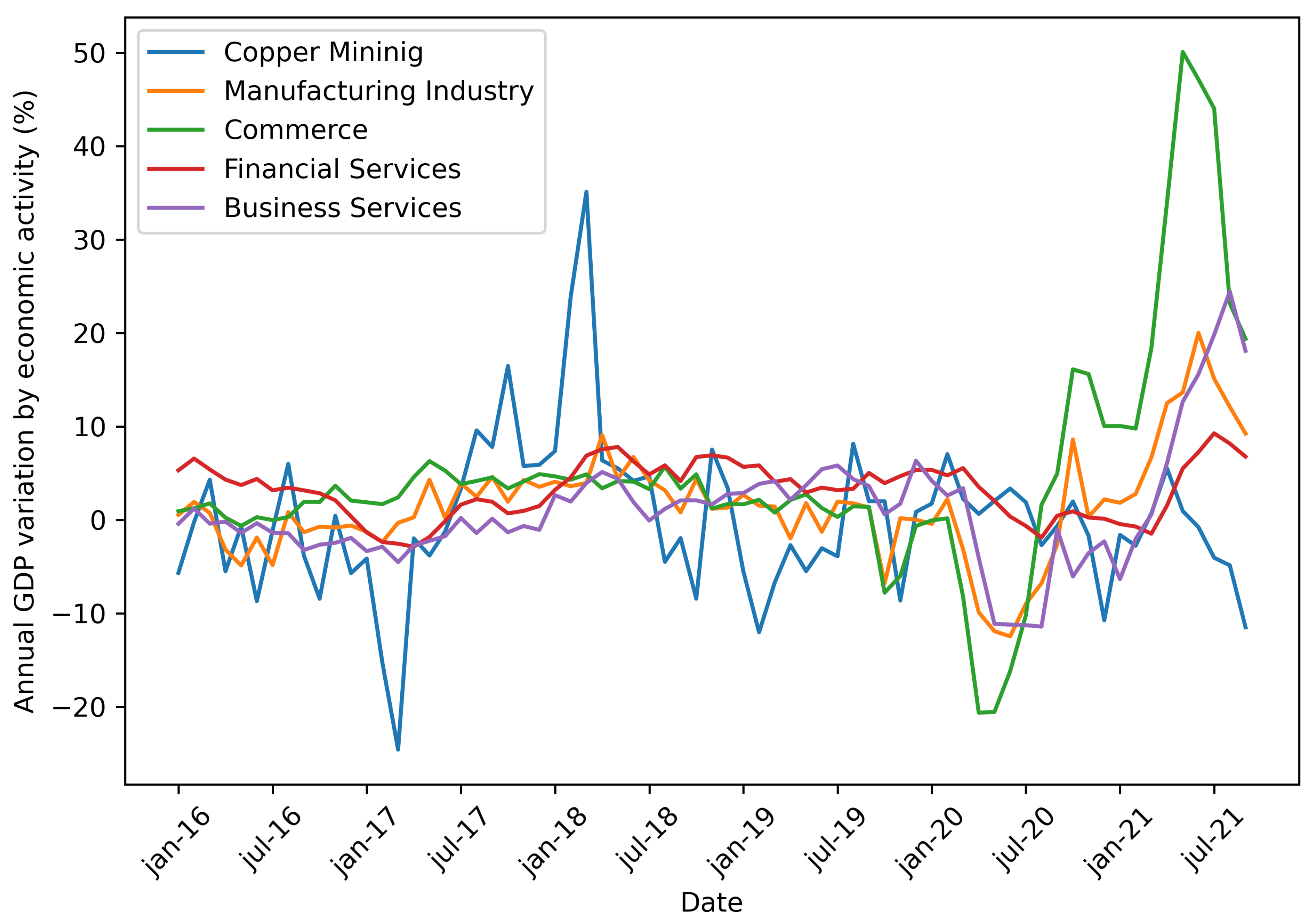
1] (BCCh) , highlights the economic repercussions caused by the pandemic on the national economic activity. For instance, in 2020, the IMACEC (Monthly index of economic activity) indicator, which measures national activity, showed a significant negative variation of 11.5% when compared to the same month of the previous year (August 2019). Furthermore, when conducting a detailed analysis using volume figures at prices from the previous year, adjusted for seasonal changes, both the mining and non-mining IMACEC reported declines of -3.6% and -12.3%, respectively. In the same period of time, the publication of the gross domestic product by economic activity (June 2020) further confirmed the severe impact of the pandemic on various sectors, as can be seen in
Figure 2. Many of them, including manufacturing (-12.5%), commerce (-16.2%), and business services (-11.2%), experienced sharp declines. However, few sectors managed to slightly surpass positive variations, such as copper mining (+3.3%) and financial services (+0.3%). These figures underscore the significant challenges faced by Chile’s economy during the pandemic and the varying degrees of resilience demonstrated by different sectors in the face of the crisis.
Amidst the pandemic crisis, the global economy has faced severe repercussions due to mobility restrictions and reduced interpersonal interactions imposed to curb the spread of the virus. As a result, it becomes of utmost importance to conduct in-depth analyses to identify and explore potential actions that can effectively minimize the economic costs borne by countries. In this context, the utilization of cluster analysis emerges as a powerful tool that enables us to delve into spatial and temporal data patterns. Through this analytical approach, valuable insights can be gleaned, aiding policymakers and decision-makers in formulating effective economic mitigation measures. By identifying clusters of regions or countries with similar economic trends and impacts, targeted and tailored strategies can be devised to alleviate the adverse effects of the crisis on different sectors and regions.
In this work we use the clustering techniques (refer to [
3,
4]), such as the k-means and the hierarchical clustering techniques,for exploring the economic consequences of possible mitigation measures, including direct transfers to households, in the context of the COVID-19 pandemic, allowing for a more nuanced understanding of the implications of various mitigation strategies. The insights derived from this research can play a pivotal role in shaping evidence-based policies and guiding decision-makers in their efforts to minimize the socio-economic repercussions of the COVID-19 pandemic on the population. As a consequence, this work holds the potential to contribute significantly to World’s response to the pandemic and could offer advises to some countries which are grappling with similar challenges.
2. Literature Review
Several studies prove that health disasters (pandemics, epidemics, etc.) not only have an impact on health but also they can affect other areas of importance. In the declared pandemic of COVID-19, we experienced a virus with the capability of conditioning the economy, impacting tourism, disrupting hospitalization levels, and implementing capacity limits in social activities. Among the consequences pointed out by scientists and experts, we harm the productivity levels of various countries, all this considering that the different governments choose to impose sanitary measures to reduce the risk of contagion. However, these measures themselves are hurting the economy, since they reduce the transaction levels, indirectly, production. The economic impact of COVID-19 has been analyzed by several authors. Ahmad et al. [
5] pointed out the possible impact that COVID-19 may have when compared to a similar type of virus, which affected China in 2002. Among the effects, they points out the impact of confinement on GDP levels not only for China given the productivity levels, but also around the world due to the restrictions on tourism resulting from the outbreak. König and Winkler [
6] presented their study on the impact of COVID-19 on economic levels in the first three quarters of 2020, for which they performed different regressions (Ordinary Least Squares and instrumental variable) in order to determine the impact on GDP given the confinement measures, where it was obtained that the more restrictive the measures are, the greater the negative impact on the economy causing an inverse relationship between mortality rate and GDP. It is known that sanitary measures are taken depending on the country and therefore these will depend on different factors associated with each country. The research by [
7] provided a better understanding of the impact of the pandemic in developing countries, where less preparedness in terms of infrastructure and equipment in the face of high infection rates has increased the impact, which has led to the need to prioritize virus mitigation measures. Jareth et al. [
8] proposed a system that allows evaluating how a given country faces the pandemic, giving it a score that goes from 0 to 100 and which is based on what the author points out as the key points to measure; such as cases per million, deaths per million, the mortality rate (percentage), hospitalization levels per million, tests performed per thousand, vaccinations per hundred people, rigor index (indicates the level of restriction of public policies) and finally, excess mortality (percentage). A predictive model was created by [
9]. This was developed using a database of economic data throughout the pandemic. The model can predict variations with a deviation of approximately 2%. The main results showed that GDP is strongly related to the market in which each country participates, together with the sanitary measures applied. Additionally, Fuente-Mella [
10] published an investigation concerning the performance of the economies of the OECD countries during the COVID-19 pandemic, they used different econometric models to predict and analyze the results. The research heavily focuses on the response that the GDP has when a defined metric(s) vary, establishing a correlation or relation between variables and the extent of the impact they may have. The results given by this model allow us to indicate comparisons between countries that belong to the OECD and the ones that don’t. However, the research by [
11] (2020) allows to understand to what extent the damage caused by the pandemic is reversible. In this study, derivatives are used to put forward the idea that COVID-19 is the product of more than one variable where the degree of impact will ultimately depend on the time of implementation of a vaccine and the effectiveness of containment.
Some authors used clustering techniques for grouping countries with similar COVID-19 effects, considering mainly the number of infected and Gross Domestic Product (GDP) variables among others. In this context the most used clustering algorithms are the
and the hierarchical cluster. In particular,
clustering is based on the shortest distance between the data and the variable centroids ([
12]), and the number of clusters has to be pre-specified. The optimal number of clusters can be determined by using some techniques proposed by Benmahdi et al. [
13]. In hierarchical clustering one can stop at any number of clusters which could be appropriate for interpreting the dendrogram [
14]. In the context of COVID-19 pandemic, Gohari et al. [
15] applied k-means method for clustering 216 countries affected by COVID-19 using mortality and incidence rates. Zarikas et al. [
16] analyzed the COVID-19 in several country by applying the hierarchical clustering algorithm to active cases, active cases per population and active cases per population and per area based on Johns Hopkins epidemiological data. Rizvi et al. [
17] presented a study aimed to cluster the countries using social, economic, health and environmental related metrics affecting the disease spread in order to implement adequate policies to control the widespread of disease. By considering 79 countries and 18 different features, the countries are grouped in 4 clusters using k-means techniques. Sadeghi et al. [
18] used hierarchical clustering analysis to evaluate COVID-19 pandemic. In particular, they cluster 180 countries into five groups using the cumulative COVID-19 fatality per day over the year and cumulative COVID-19 cases per million population per day over the half-month period. In order to cluster time series with temporal differences, the dynamic time warping distance measure proposed by [
19] have been often used in literature jointly with the clustering methods. Yavuz et al. [
20] implemented time-series clustering with the dynamic time warping method for world countries by using all available daily confirmed cases, recovered cases, and death data, after adjusting for population. Their results evidenced that European, North and South American continents had homogeneous structures regarding the number of daily confirmed cases and relatively more heterogeneous regarding the daily number of recoveries. The the dynamic time warping distance and hierarchical cluster is also used by [
21] to cluster time series of daily new cases and deaths from different countries into four patterns. They found that geographic factors are important but not decisive for the pandemic development, and that the age population may also influence the formation of cluster patterns.
Finally, Mahmoudi et al. [
22] propose the use of fuzzy clustering for studying the distributions of the spread rate of Covid-19 in Unites States America, Spain, Italy, Germany, United Kingdom, France, and Iran. The results showed that Covid-19 spreading in Spain and Italy was approximately similar but different from other countries.
3. Methods
The methodology employed in this study is centered around the application clustering techniques with the main aim to assess the impact of the SARS-CoV-2 pandemic on selected OECD countries. In order to do this, we consider the Gross Domestic Product (GDP), and the economic mitigation measures implemented by these nations. Additionally, we consider the cumulative infection rate per 100,000 inhabitants within the target population from the onset of the pandemic through the conclusion of 2021.
3.1. Data sample
In this study, we considered global and national data. For the global analysis, we selected variables collected by 52 countries (38 OECD member countries and 14 not OECD members), represented in
Table 1, during the years 2020 and 2021. In particular, for each country, we considered: (i) the infection rate for 100,000 inhabitants (
) for each country [
24];(ii) the variation of GDP (Gross Domestic Product) for the period 2020 and 2021 for each country, taking as basis the 2019; (iii) the number of mitigation measures [
26] that countries took into account for years 2020 and 2021. For the GDP variation, two folds were considered: the variation between 2019-2020 and between 2019-2021, by extracting data from [
25] and calculating the variation over each period as follows:
Regarding the mitigation measures, while [
27] used information until 2020, in this study we updated the database up to 2022 in order to incorporate all the financial policy measures. In particular, we use simple count of the total measures taken by each country in both years 2020 and 2021.
In the context of the National case, we considered three time series measurements. Firstly, we examined the Chilean daily infection rate per 100,000 inhabitants. This infection rate was calculated by multiplying the number of daily cases by 100,000 and dividing by the total Chilean population. Secondly, we investigated the closing prices of the daily Chilean stock market index, known as IPSA [
28]. This index effectively tracks the performance of the largest Chilean companies. The third variable to study is the daily interest rate, which is given by the Central Bank of Chile [
29]. It’s important to note that the data for the IPSA and the daily interest rate, were available exclusively for business days. Therefore, to ensure consistency and comparability across these variables, we measured the percentage variation between each data point, facilitating meaningful comparisons into the dynamics of the data. For example, the percentage variation of IPSA (
) was calculated as follows:
3.2. Clustering
As we mentioned in the previous subsections, we used two different databases to analyze the pandemic. In order to give a detailed description of how groups of countries can gather together based on similar course of actions, related to economical variables, we used the classical clustering techniques, i.e. k-means and hierarchical clustering.
K-means clustering is a part of a unsupervised learning technique from machine learning [
12,
30,
31]. It begins partitioning a dataset into
K distinct clusters based on data point similarity. It starts by randomly selecting K initial cluster centroids and assigns each data point to the nearest centroid. Centroids then update iteratively as the mean of their assigned data points. This process continues until centroids stabilize. In order to find the appropiate
K value, we employed three different methods that will be shortly describe in the following subsection.
Hierarchical clustering is also a unsupervised learning technique from machine learning [
32], which form clusters according on agglomerative (bottom-up) or divisive (top-down) approach. In this work we will consider the agglomerative method where the clustering process starts by considering each data point as an individual cluster and then iteratively merges the closest clusters into larger ones. This process continues until all data points belong to a single cluster or meet specific stopping criteria. Hierarchical clustering produces a dendrogram, a tree-like structure, which reveals the hierarchy of cluster relationships. It doesn’t require specifying the number of clusters beforehand, making it versatile for exploring data structures.
Dynamic Time Warping (DTW) is an algorithm employed for assessing the similarity between time sequences that may exhibit variations in both time and speed [
33]. Its primary purpose is to identify patterns by measuring the temporal distance between data points in the sequence under consideration and the centroids of one or more clusters. It accomplishes this by selecting various points from these sequences at different time intervals and grouping them based on the minimal distance to the centroids of the clusters to be determined during analysis (for details see [
34]).
3.3. Number of cluster’s estimation methods
A crucial step in cluster analysis is related to the selection of the optimal number of clusters. In this work we used the elbow method, The Silhouette method, and the Gap-Statistics. The elbow method, which can be traced back to [
35], is a heuristic algorithm that analyzes the within-cluster sum of squares across various cluster numbers. The "elbow point" indicates optimal clusters where reduction slows, balancing variance capture and fragmentation prevention. The Silhouette method, proposed by [
36], assesses clustering by cohesion and separation distances. Individual scores create averages for various cluster counts, revealing optimal clusters with high cohesion and separation balance. The third method we consider is called the Gap-Statistics, it is based on a Statistic proposed by [
37], the method consist in determine clusters by comparing actual data’s clustering to random data, revealing optimal clusters without biases toward excessive clusters or noisy data.
4. Results
4.1. Exploratory data analysis
In this section we present some summary statistics for the Global dataset, as shown in
Table 2. Notably, we observe a significant standard deviation for the variables related to Measures, this variability can be attributed to the inclusion of 14 countries that reported no economic mitigation measures for both years.
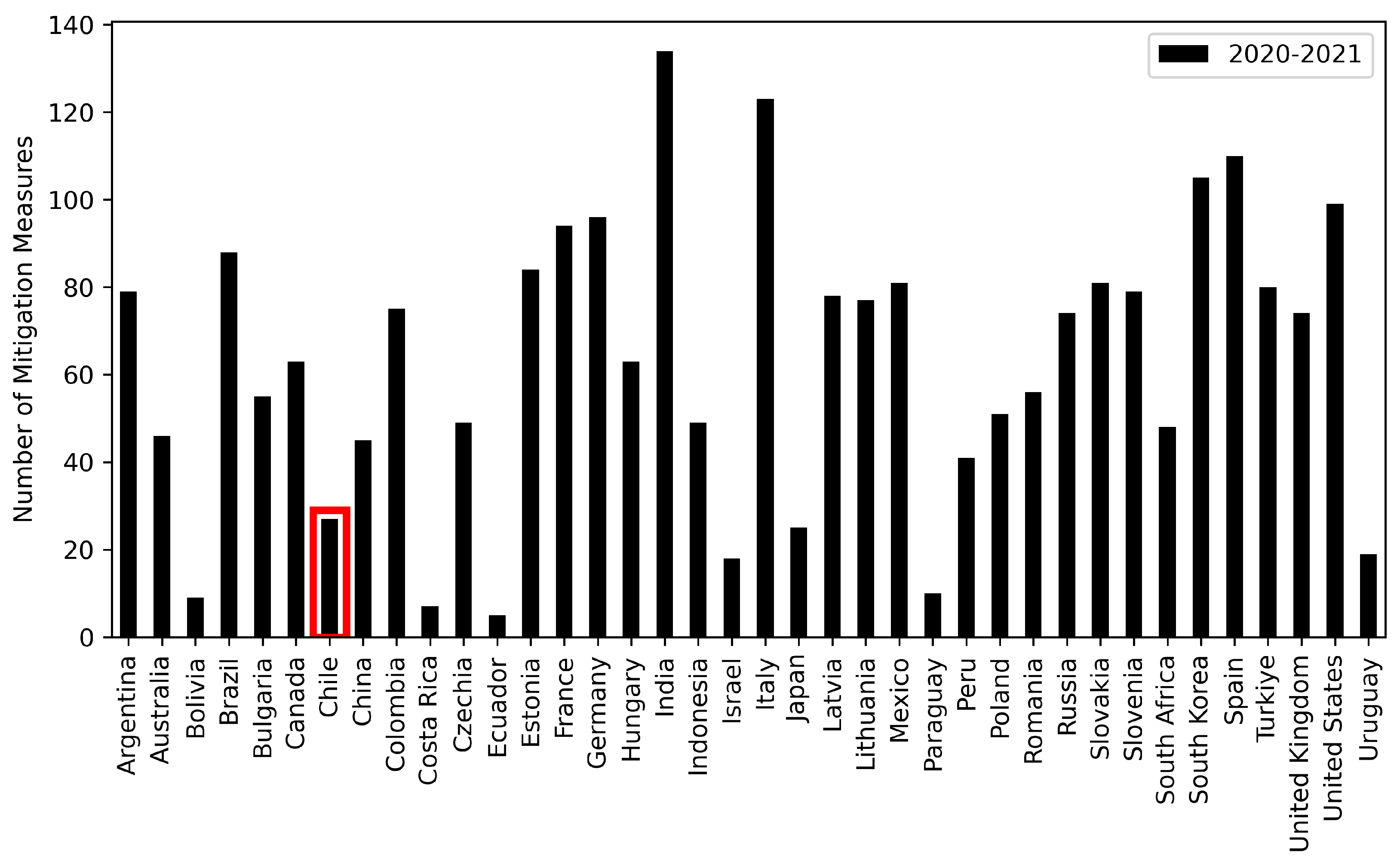
Figure 3 represents the number of economical mitigation policy measures, related to banking sector, liquidity/funding, financial markets, insolvency, payment systems, etc. Focusing on Chile (the bar within red rectangle in
Figure 3), we can see that it falls below the mean value and ranks lower than several other American countries. Additionally, in
Figure 3, we observe that the three countries with the highest number of mitigation policy measures, in descending order, are India, Italy, and Spain.
Based on the variable Infected in
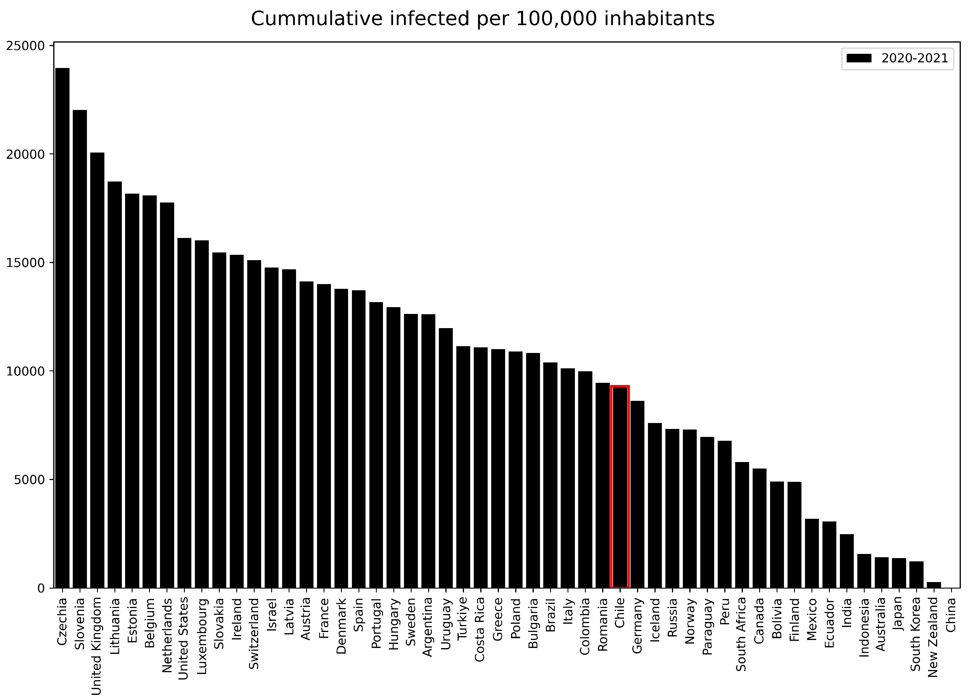
Table 2, which represent the accumulated infection rate until 2021, we notice that minimum value is 91 which belong to China, represented by the last bar on the right of
Figure 4. This phenomenon can be elucidated by considering that infection rates are adjusted by the respective population size. In this regard, China stands out as the world’s most populous country, as documented in [
24]. It is noteworthy that India, the second-most populous nation, significantly surpasses China’s infection rate.
Shifting our focus to Chile, we find that it exhibits an infection rate below the mean (9258.02), which is illustrated in
Table 2. Furthermore, in
Figure 4, Chile is highlighted within a red box, signifying its position as the thirty-third country in descending order of cumulative infections per 100,000 inhabitants. Interestingly, Chile’s rate exceeds that of five other Latin American countries, namely Paraguay, Peru, Bolivia, Mexico, and Ecuador. An additional noteworthy observation arises from
Figure 4, where we see that nine out of the top ten countries with the highest cumulative infections per 100,000 population belong to Europe with exception of United States (eighth position).
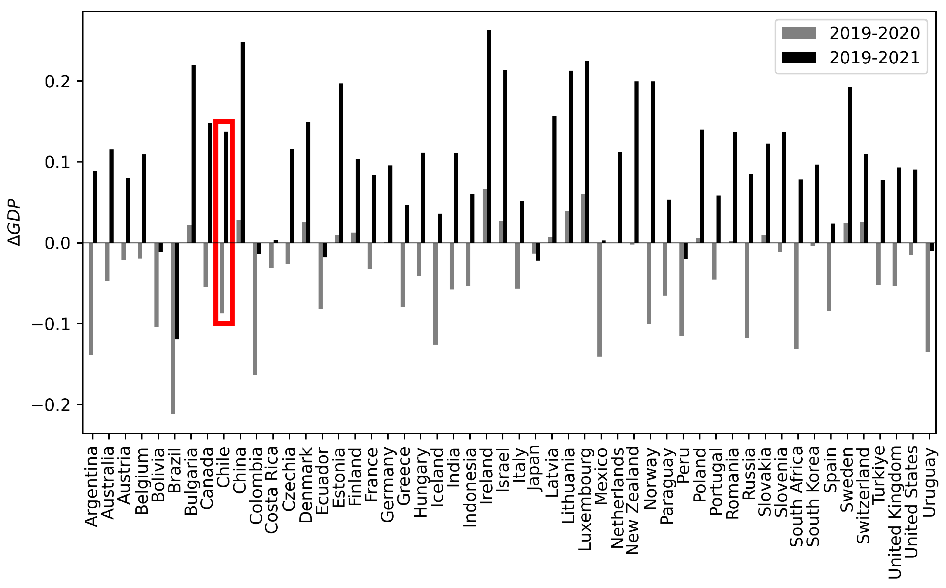
The analysis of GDP variation for the periods 2019-2020, and 2019-2021 is represented in
Table 2 by the variables
and
, respectively. A comparative analysis of these two-year variations underscores the evident negative impact of the Covid-19 pandemic on global GDP values. The mean value for these variables is consistently negative, and GDP values remain negative above the median and until at least the 69th percentile (-0.0002862). Notably, in 2021, there is a visible rebound reflected in the positive mean and a positive 25th percentile. A more detailed country-level analysis in
Figure 5 provides valuable insights into the diverse behaviors of nations. The gray and black bars in this figure represent
and
respectively. Within this figure, an interesting situation becomes evident: several countries did not experience a negative GDP variation for both comparative years, with the majority of them being European nations, except for China, Israel, and New Zealand. Conversely, there is a group of countries that encountered negative GDP variations for both years, encompassing nearly all Latin American countries, such as Bolivia, Brazil, Colombia, Ecuador, Peru, Uruguay, with Japan being the exception. Notably, Chile, along with Argentina, Costa Rica, and Paraguay, stands out as the only Latin American countries that managed to rebound in 2021, showing a positive trend.
4.2. Selection of the number of cluster
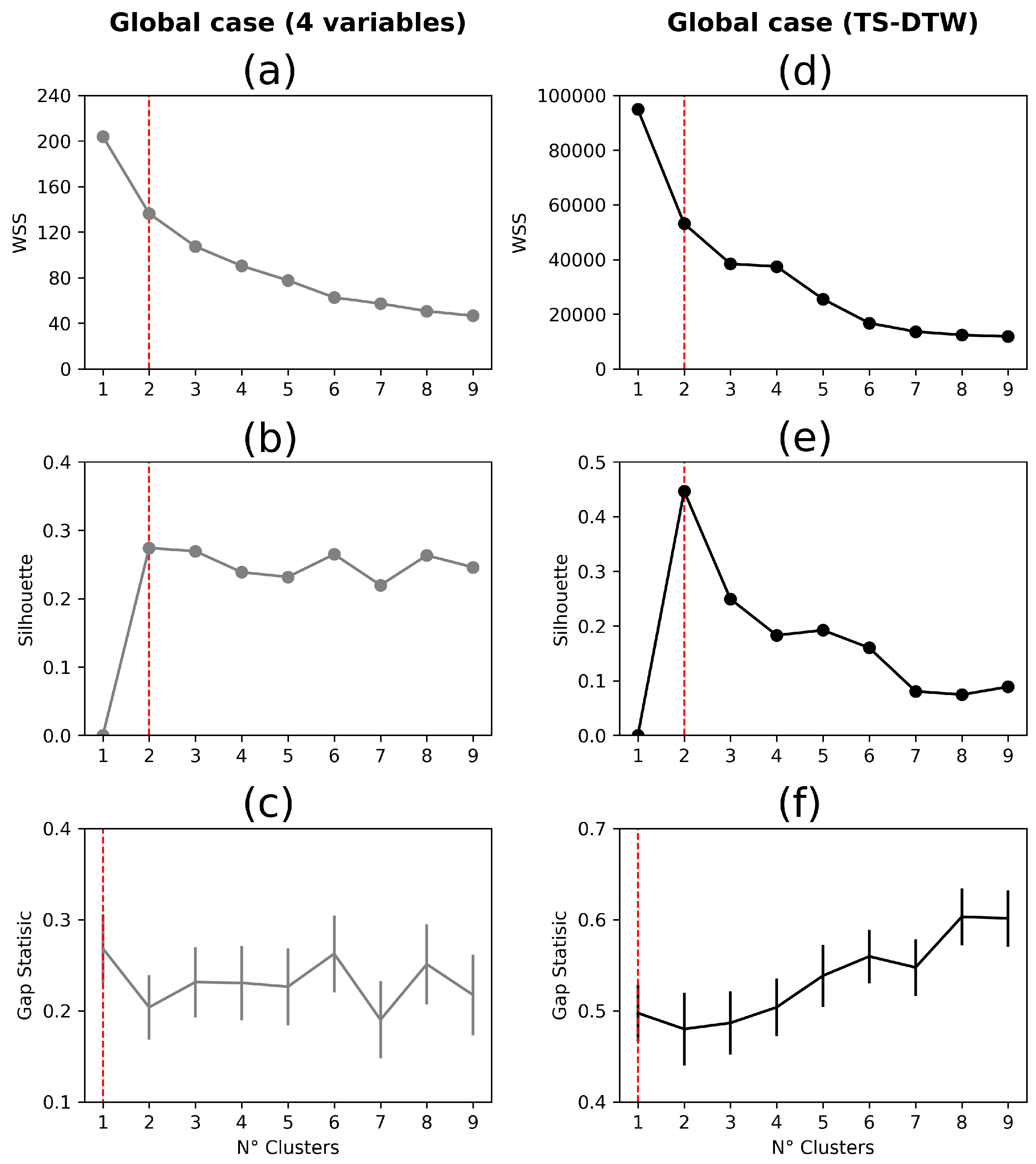
In
Figure 6, we present some methods for selecting the optimal number of clusters, a critical step in our analysis. In particular, the decision of how many clusters to use relies on a consensus derived from the collective insights of various methodologies previously outlined, including the elbow method (panels a and d), silhouette analysis (panels b and e), and Gap-Statistic (panels c and e). The aim is to strike a balance in identifying a reasonable number of clusters that effectively unveil the inherent patterns within the global dataset. In our analysis, we have prominently denoted
with a segmented vertical red line, aligning with both the elbow method’s Weighted Sum of Squares (WSS) and the Silhouette method. Despite the Gap-Statistic points towards an optimum at
, signifying unclustered data, we opt to heed the collective recommendation of the elbow method and Silhouette analysis, as both concur on
as the most appropriate choice for clustering countries’ behaviors. This consensus-driven decision ensures that our clustering approach effectively encapsulates the underlying dynamics of the dataset, enhancing the reliability of our findings and interpretations.
The second column of
Figure 6 determines the appropriate number of clusters for the global database, specifically concerning the daily infected rate per 100,000 inhabitants. In this scenario, we utilized the hierarchical clustering method with Dynamic Time Warping (DTW) as the distance metric to cluster the data from 52 countries. Again, we found an alignment among the elbow method’s Weighted Sum of Squares (WSS) and the Silhouette method. K=2 emerged as the choice across this two methodologies. This consensus on the optimal number of clusters holds substantial significance as it underpins the comparison between two perspectives of the pandemic.
4.3. Formation of Two Significant Clusters Using Static Data from Countries
Utilizing data related to the pandemic’s development, mitigation policies, GDP variations from 2019-2020, 2019-2021 and cumulative infection rates until the end of 2021, we constructed a comprehensive database for each country. Subsequently, we conducted two classical data clustering analyses, hierarchical and k-means, using the R Statistical Software [
40].
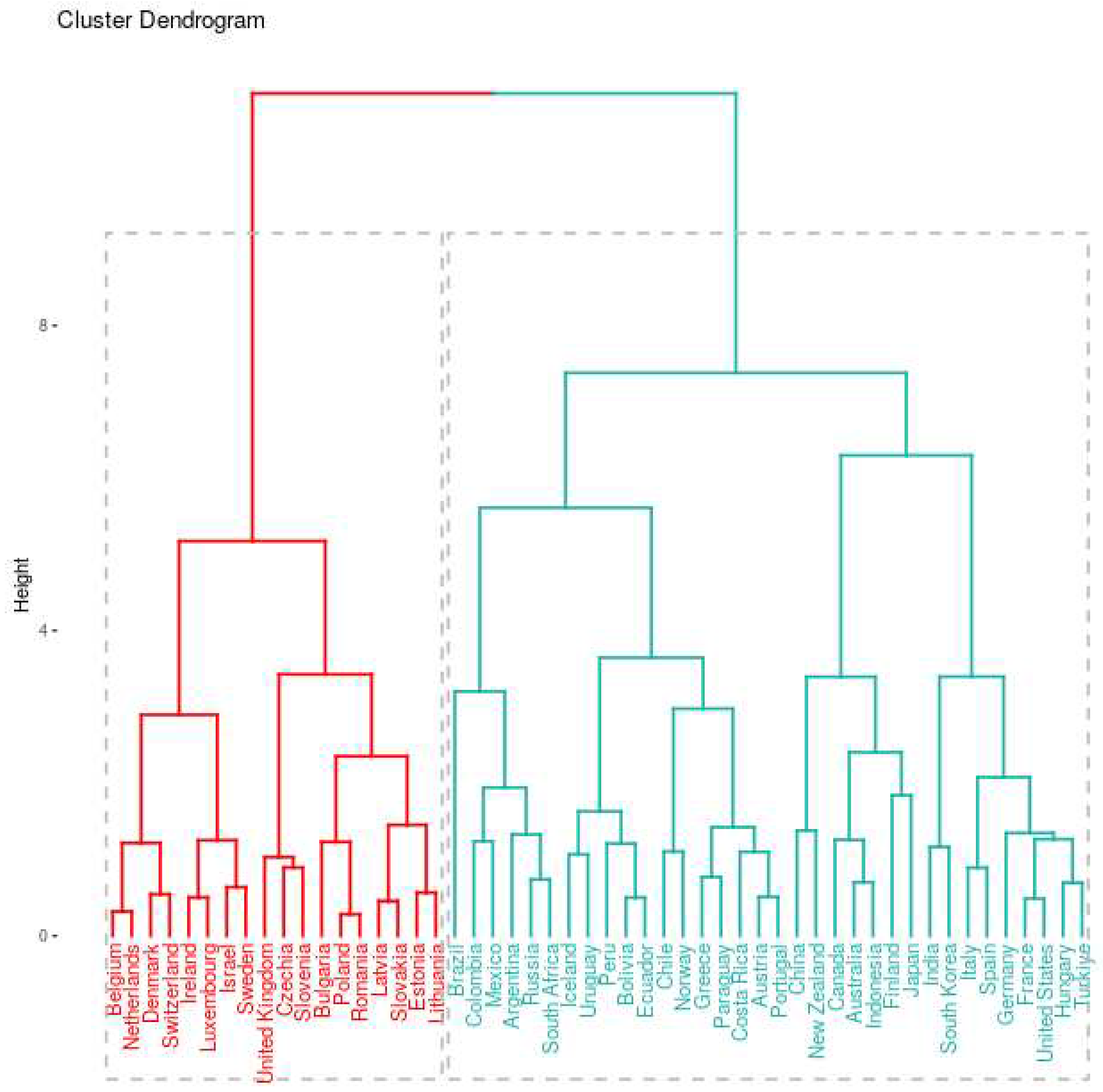
Figure 7 illustrates the hierarchical clustering dendrogram, revealing the formation of two prominent clusters: one consisting of 18 countries (depicted in red) and the other comprising 34 countries (represented in cyan). This analysis allowed us to group countries based on shared characteristics, shedding light on the dynamics of the pandemic’s impact on different nations, their economic performance, and policy responses.
In
Figure 7, an interesting pattern arises as we observe that all Latin American countries are clustered within the cyan group. The hierarchical cluster analysis not only shows the arrangement of countries but also offers valuable insights into the similarities among data points. Notably, the red cluster primarily encompasses European countries, with the sole exception being Israel. Furthermore, it’s important to highlight that within the smaller cluster, the majority of countries belong to Central Europe (10), with the remaining four representing Western Europe.
Another pattern that emerges from
Figure 7 pertains to the geographical distribution of countries. On one side, we find all countries from Asia and Oceania within the cyan cluster. However, upon closer examination of the dendrogram, it becomes evident that if we were to partition the cyan cluster into two, it would lead to a more distinct alignment with these countries. In such a scenario, the other cluster would encompass all the Latin American countries. This potential division of the cyan cluster offers an intriguing opportunity for further investigation, providing insights into the factors influencing these groupings.
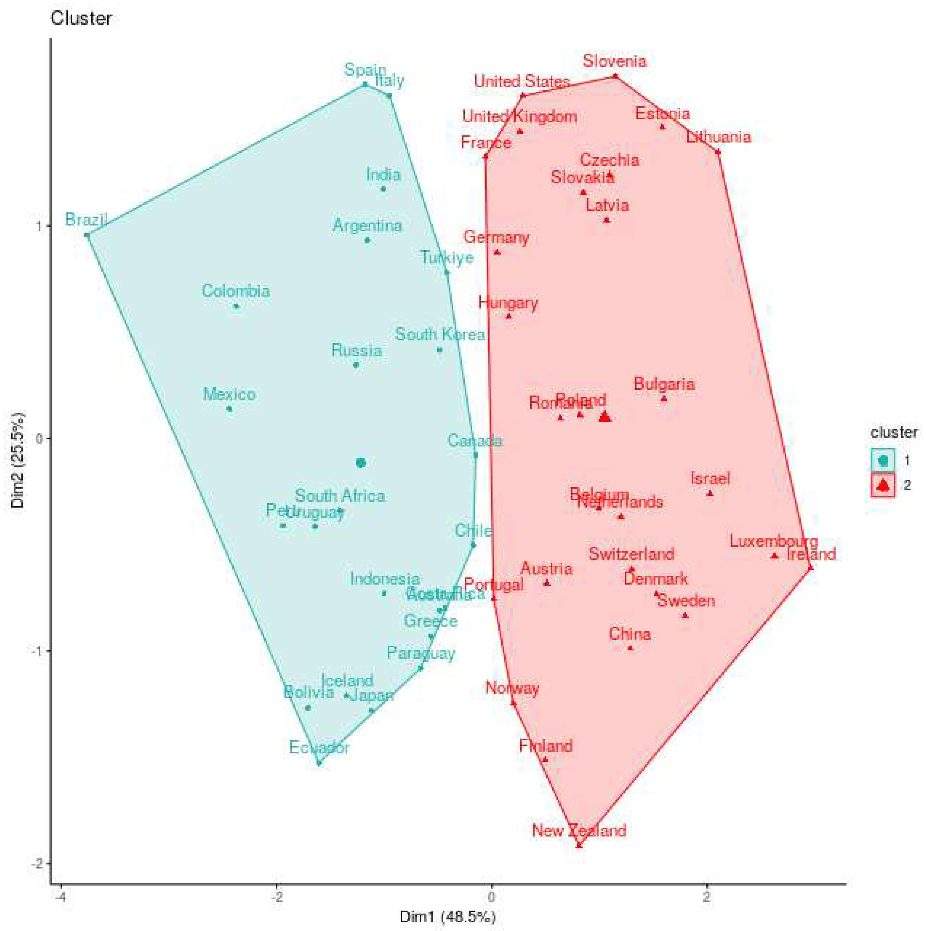
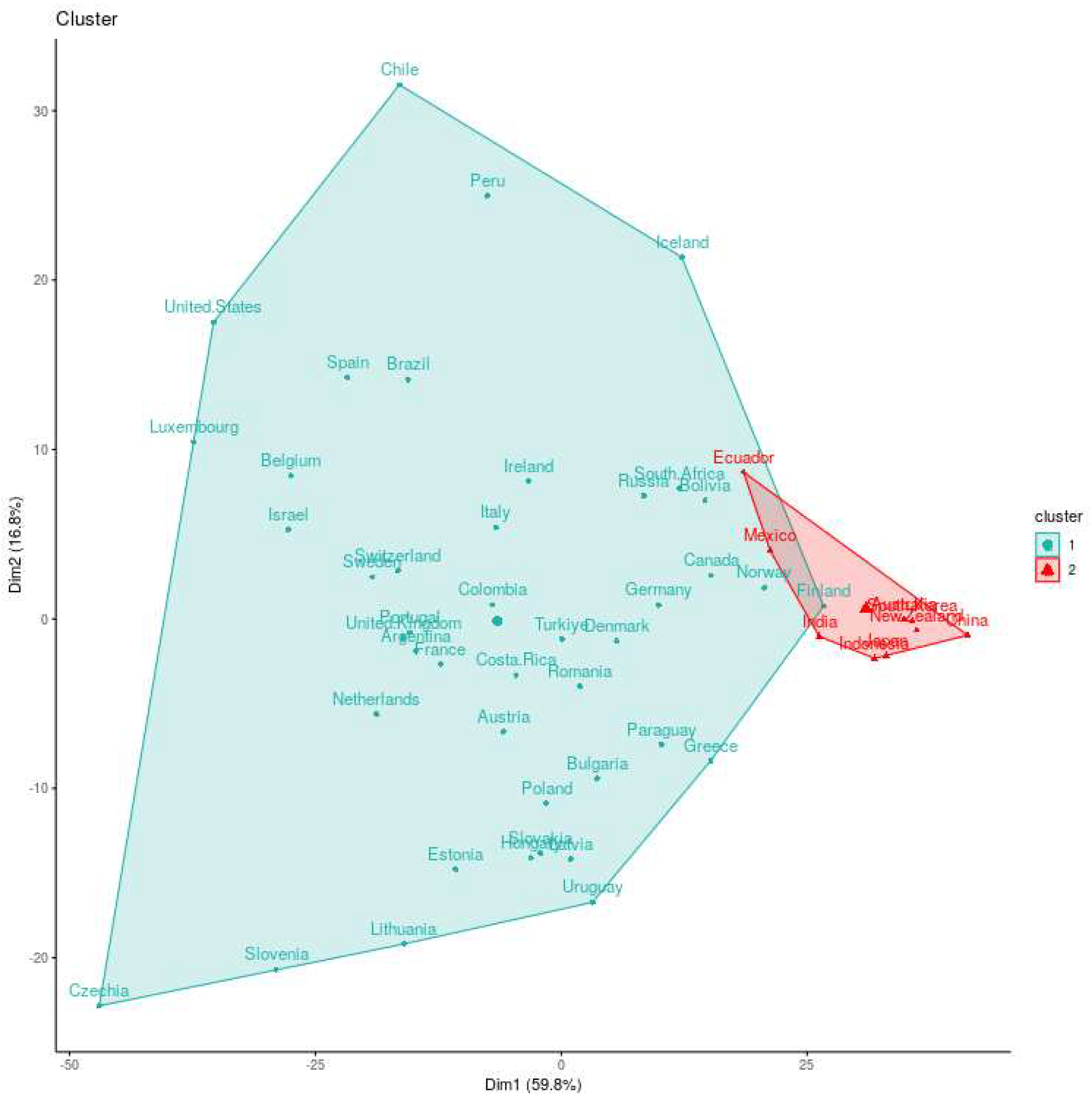
When we examine the k-means clustering using Principal Component Analysis (PCA) by projecting the countries into the first two components in
Figure 8, we found that eigth countries that were initially categorized in the cyan cluster in hierarchical clustering depicted on
Figure 7 are reassigned to a different cluster in the k-means analysis. This finding underscores the influence of the clustering method on how countries are grouped and categorized, revealing the sensitivity of the results to the chosen methodology.
However, it’s notable that all the countries incorporated into the red cluster in
Figure 8 are primarily clustered along the left boundary of the convex hull formed by the countries in this group. Importantly, the majority of the countries newly added to the red cluster are of European origin, with exceptions such as the United States, China, and New Zealand. Another noteworthy feature of this PCA projection is its capacity to reveal that all the countries belonging to the red cluster in
Figure 7 are collectively positioned towards the right side of the convex hull illustrated in
Figure 8. This observation highlights an interesting geographical and structural distribution within the red cluster.
4.4. Clustering the Evolution of Infection Rates in Countries using Dynamic Time Warping (DTW)
The global spread of COVID-19 originated in China and subsequently affected countries worldwide, leading to a common issue in analyzing time series data, i.e. the absence of a consistent starting point in time for each country’s pandemic experience. To address this issue, Dynamic Time Warping (DTW) method as a distance function, emerges as an ideal tool for handling the variations in the begin of the COVID-19 outbreak in different regions. The main advantages of DTW, when compared to other distance metrics is that we can better analyze and understand the global dynamics of the COVID-19 pandemic, accounting for the temporal disparities in the spread of the virus and capturing complex patterns that define its progression. In
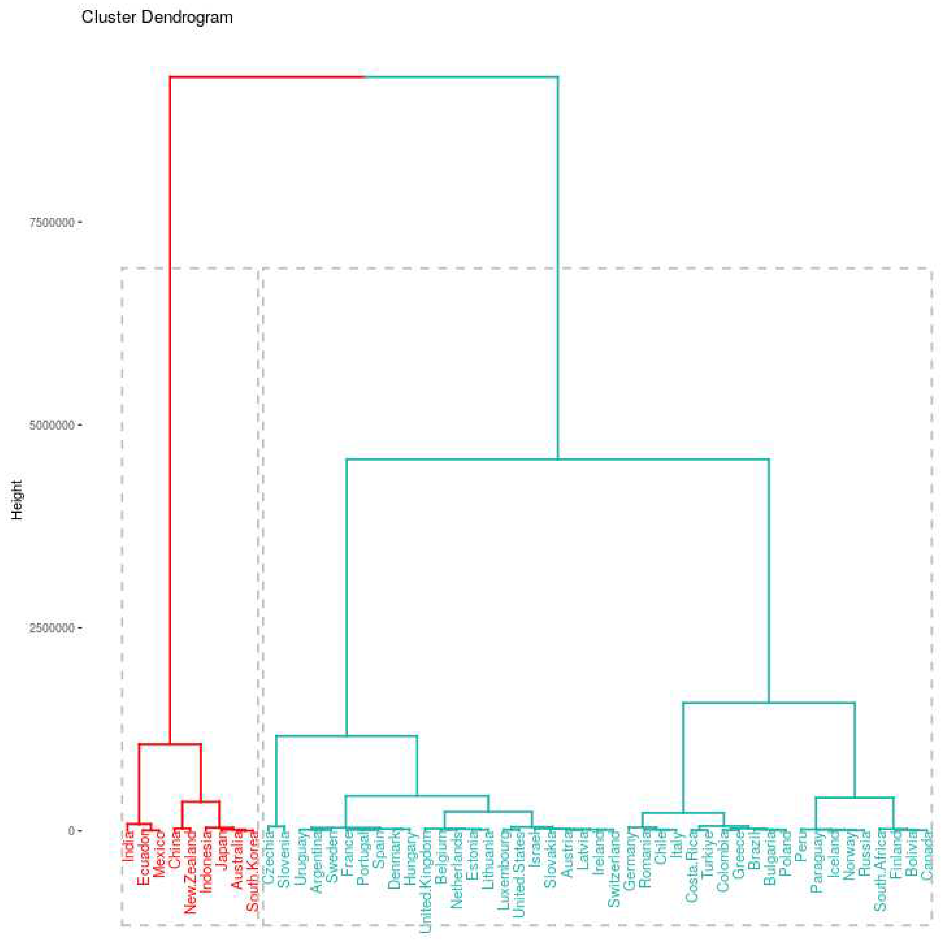
Figure 9, we employed DTW as a distance measure between the time series of infection rates for each country spanning from 2020 to 2021. We use this DTW-based approach within the context of Hierarchical clustering.
In
Figure 9, it’s clear that the red cluster encompasses fewer countries compared to the initial database analyzed using both clustering methods. This reduction in the number of countries highlights a consistent pattern when comparing the composition of the red clusters in
Figure 7 and
Figure 8 with
Figure 9. Notably, the countries within this cluster align together across the two figures, maintaining a degree of consistence.
A noteworthy outcome of this clustering analysis is the prevalence of countries from Asia and Oceania within the red cluster. However, exceptions exist, with Mexico and Ecuador representing Latin American countries. An intriguing observation arises when examining the dendrogram of the red cluster, revealing that Mexico and Ecuador share a subgroup with India, while the remaining countries form a distinct group. This finding aligns with the grouping pattern observed in
Figure 7, where Latin American countries (Mexico and Ecuador) were clustered together, and countries from Asia and Oceania were grouped separately. In order to provide an alternative view on the clustering characterization, we projected the clusters onto the first two principal components, as illustrated in
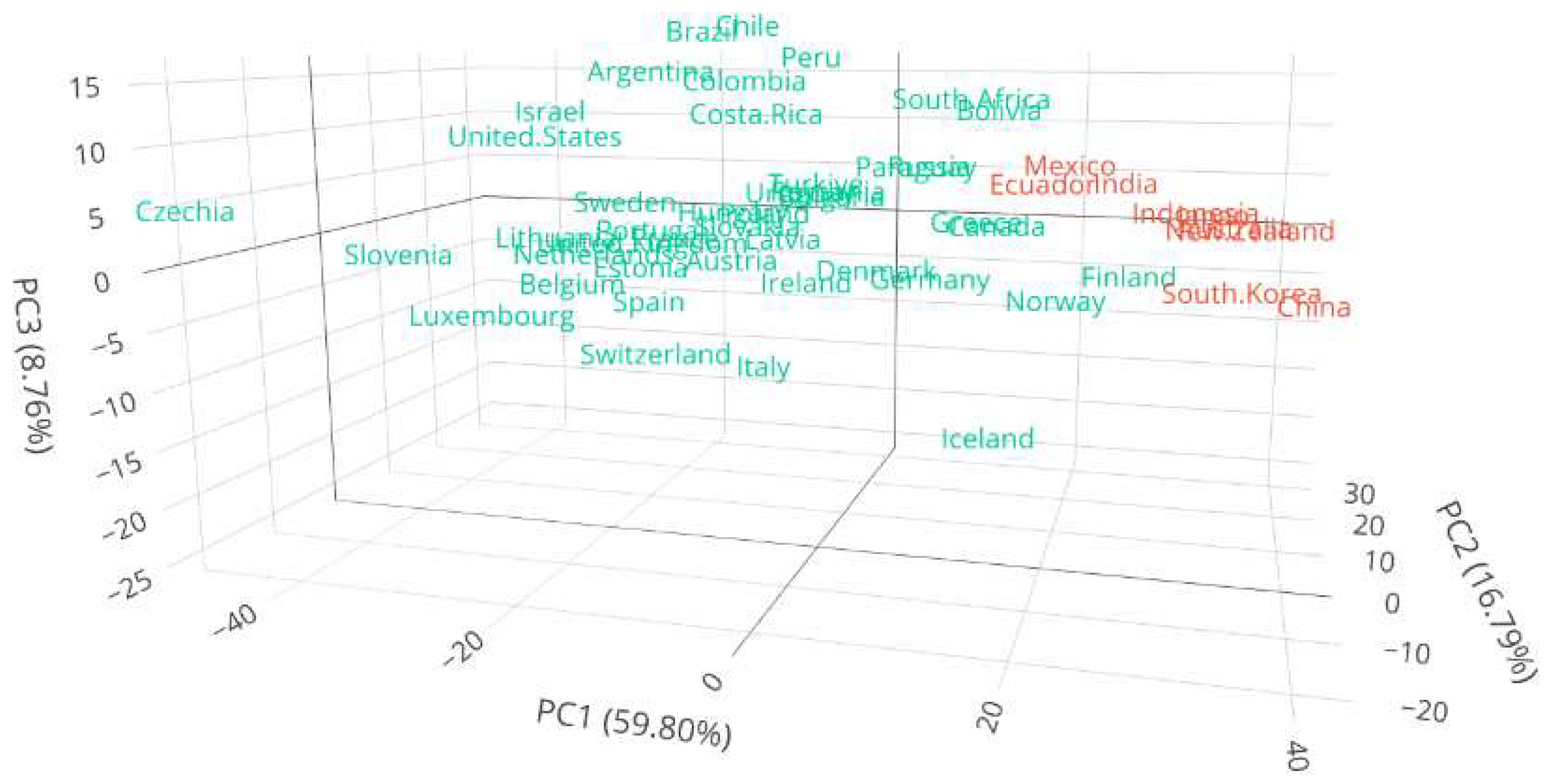
Figure 10. In this visualization, the red cluster is situated on the right side of the figure. Notably, there is an overlap between the two clusters in this projection. This overlap can be addressed by further projecting our countries, incorporating a third principal component, as it is shown in
Figure 11. The projection into the first three principal components not only reveals a more accurate separation of the two groups but also provides a deeper understanding of how countries are distributed within this three-dimensional subspace. It’s worth noting that this subspace encapsulates over 80% of the total explained variance. Additionally,
Figure 11 also shows that the cluster belong to the boundary of the dataset. We also notice that this cluster includes countries like China, Japan, India, and Australia, which experienced active cases within the first thirty days of the pandemic’s onset.
Compared to the initial cluster analysis, the utilization of DTW in
Figure 9 unveils a notable distinction. It shows that all European countries are consolidated within a single cluster, i.e. cyan group, whereas the selection of the number of clusters in
Figure 3 suggests the presence of two distinct groups, a closer examination of the dendrogram in
Figure 9 may indicate the potential existence of three clusters. In this scenario, the group formation shows an interesting pattern, where seven Latin American countries are positioned on the right branch of the dendrogram, while Argentina and Uruguay find their place within the middle cluster. It’s essential to note that the two countries with the highest infection rates, depicted in
Figure 4, namely Czechia and Slovenia, share a common branch in the dendrogram.
4.5. Chilean case
This section aims to analyze more deeply how COVID-19 affected certain economic variables in Chile. By having a more detailed analysis of the Chilean case, it will be possible to highlight specific actions that helped from a practical point of view to mitigate the complications caused by the pandemic, e.g., if the COVID-19 pandemic has long-term structural effects on individual consumption behavior.
The International Federation of Pension Fund Administrators: [
41], published a study in which it analyzes the impact of the pandemic on employment, the number of contributors, and the collection of pension funds in different countries of the world, indicating that only three countries in the world (Australia, Chile and Peru) allowed withdrawals from mandatory pension funds. In contrast, other countries allowed withdrawals from voluntary savings accounts as a measure adopted by governments to help them cope with the crisis.
In the case of Chile, three withdrawals from mandatory pension funds were authorized (Laws: N° 21.248, N° 21.295, N° 21.330), which could be a total for those with a balance of less than 35 UF (approx. 1,346 USD) or 10% with a cap of 150 UF (approx. 5,767 USD), with only the second withdrawal being subject to tax for those with monthly income of more than CL$1,500,000 (approx. 1,890 USD). These withdrawals were approved by three constitutional reforms at different times. The total withdrawal amounts to 50,334 million dollars in less than 12 months, reaching a total of 25,527,807 withdrawals by the inhabitants of Chile.
The above-mentioned is important to consider since injecting a large amount of money into the Chilean economy would affect different variables such as inflation, interest rates, and the capital market. This finally has repercussions in the different measures that must be taken to balance the economy during and after having faced the pandemic. Understanding that the measures taken by the different countries are not homogeneous, we can analyze certain variables that give us some guidelines on the country’s economic direction. Therefore, we analyzed the interest rate, infection rate, and market profitability.
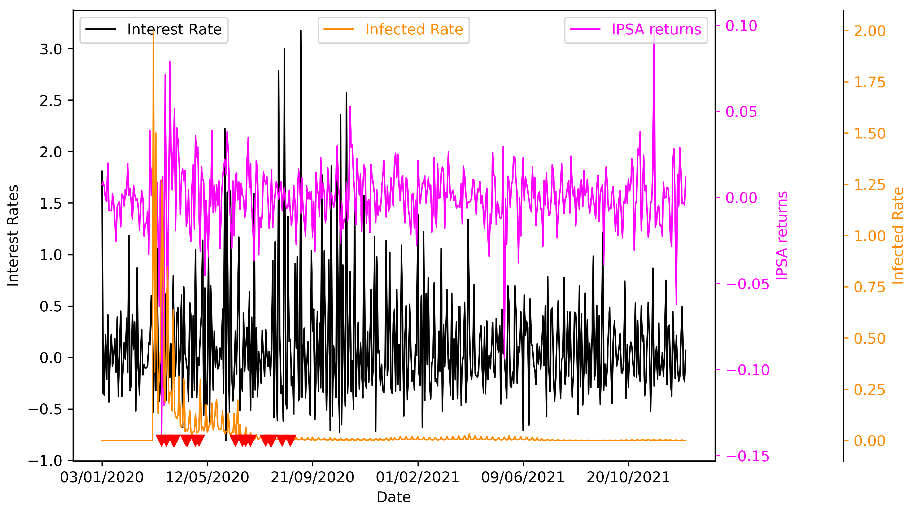
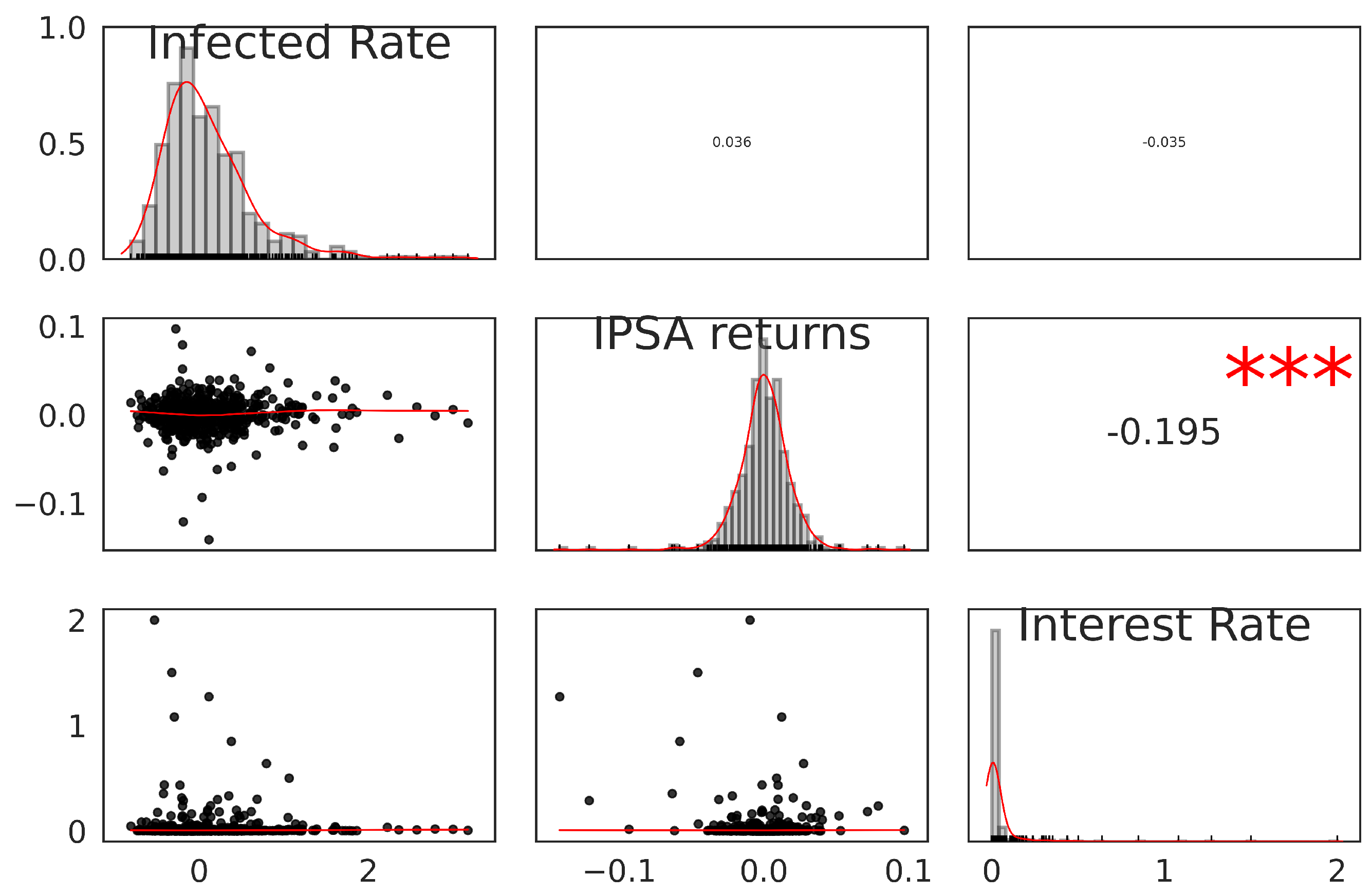
Figure 12 shows the three variables used to analyze the Chilean case, and we can see in orange the series representing the rate of COVID-19 infections, showing a reasonably marked pick in the periods that most affected Chile. The following two series, the interest rate in black and the market return represented by the IPSA stock market indicator (for details of IPSA, see [
42,
43] and reference therein) in purple, represent a certain degree of positive correlation, which we can see visually.
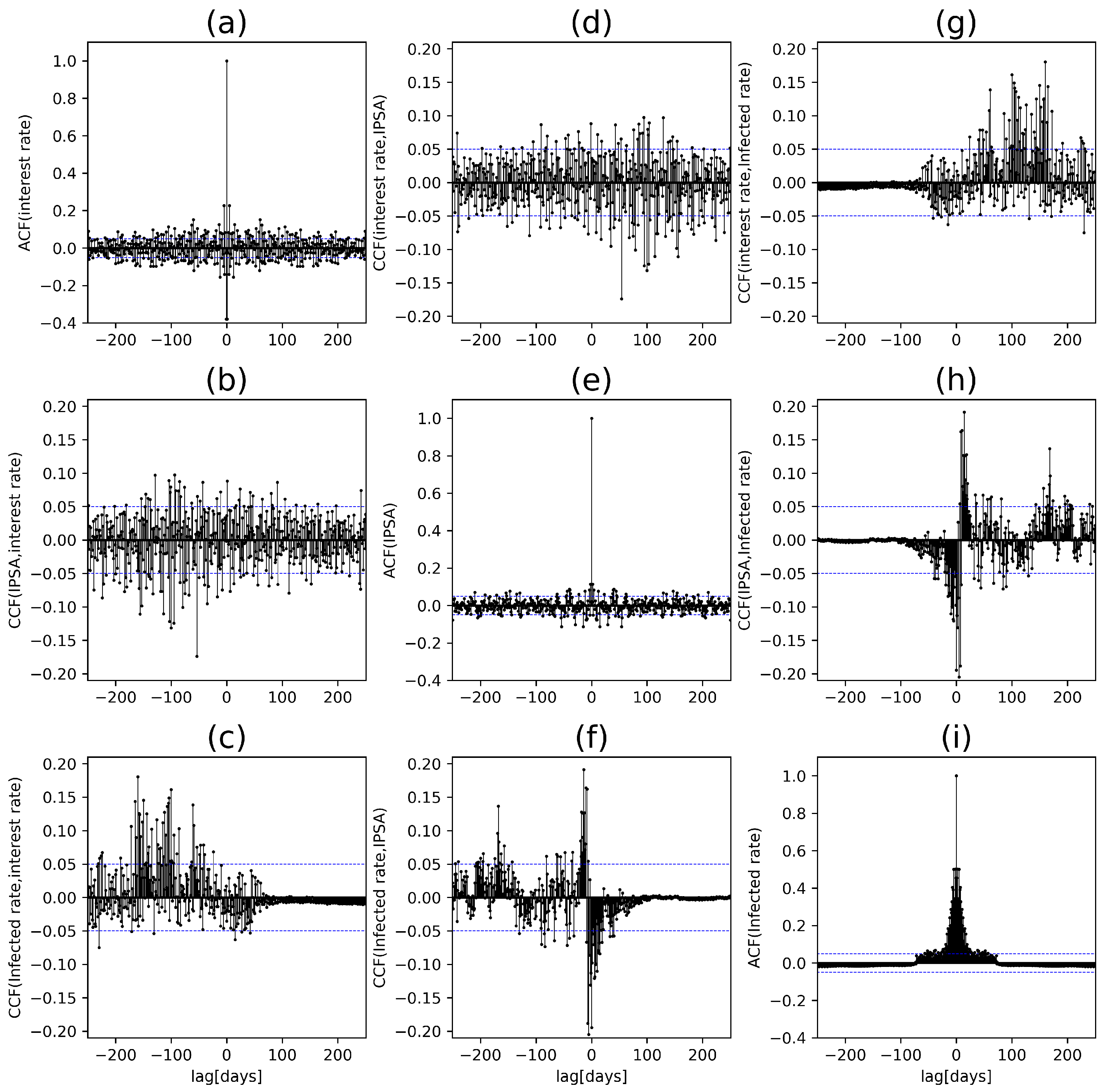
As we can see in
Figure 14 and
Table 3 we analyze the Cross-Correlation to track the movements between the variables. The three time series are daily and from January 2020 to December 2021. As expected, the interest rate is correlated with IPSA; according to economic theory, they should have a negative correlation because when interest rates increase, companies may have less money to invest back into the company due to higher borrowing costs, which can reduce cash flow stability and put pressure on share prices. However, as we can see, this is positive in certain lags, which could occur due to the sudden increase in the purchasing power of people due to the different economic aids. Specifically, for this case, we can observe a maximum lag of 54 days, which would imply a mismatch between the monetary policy decision and the reaction of the capital market. This can also be seen in the
Figure 13, which contains a negative correlation.
On the other hand, there is no significant correlation between the infected rate with the IPSA and the interest rate, as shown in
Figure 13. However, we can evidence in
Table 3 a maximum lag of 160 days between the infected rate and the interest rate and a slight maximum lag of 5 days between the infected rate and the IPSA.
5. Conclusions
The impact of COVID-19 caused a significant shock to the economies of all countries in the world. In just one year, the effects could be seen in the lower projections of the different economic indicators, with figures that had not been recorded for a long time. The International Monetary Fund recommended adopting economic measures that could halt this slowdown, which were adopted in several countries to help people who lost their jobs and who, as time went by, found themselves increasingly submerged in debt.
The results of the measures were remarkable during 2021 when several economic activities had favorable variations. These are shown in the countries’ GDP, which showed a rebound compared to 2020, which was difficult due to the freezing of different economies. However, it must be recognized that the measures are temporary and that the 2020 scenarios could reoccur if work does not continue on measures to activate the economy. It is also essential to continue studying cost-effective measures to avoid future economic crises due to pandemics and natural disasters, as this could trigger a deep economic crisis in several Latin American countries that may not be able to withstand a new downturn in their economic activities.
This work has explored various dimensions of the COVID-19 pandemic’s impact on countries worldwide. We began by investigating the economic measures taken in response to the pandemic, highlighting the diversity of policy responses among countries. Despite Chile’s relatively low number of economic measures, we observed other countries that took no economic measures at all. Notably, India, Italy, and Spain were at the forefront of implementing mitigation policies.
Our cluster formation analysis incorporated various static data parameters, encompassing aspects related to pandemic development, mitigation policies, GDP variations, and cumulative infection rates. Through the application of hierarchical and k-means clustering methods, we were able to delineate two distinct clusters within our dataset. An interesting finding emerged as Latin American countries exhibited a notable propensity to cluster together, forming a cohesive subgroup within one of the identified clusters. Similarly, Asian and Oceania countries tended to coalesce within the same cluster, further emphasizing regional patterns. This study carries out significant findings by extending the analytical framework proposed by previous researchers (see, [
20] for example), exploring not only the epidemiological component but also the economic and political implications of infectious diseases. The congruence in outcomes between the two analytical perspectives is particularly noteworthy.
We employed Dynamic Time Warping as a distance metric in hierarchical clustering to address the temporal disparities in the pandemic’s spread. This approach facilitated the alignment of infection rate time series, overcoming challenges related to varying pandemic onset dates. While the number of countries in the smaller cluster previously described decreased its size, there was consistency when comparing the countries in this cluster in the two different analyses. The projection of clusters onto the first three principal components further enhanced our understanding, revealing a more precise separation of groups and providing deeper insights into country distribution within a three-dimensional space.
The Chilean case analysis allows us to understand better the relationship between the main economic variables and how they react to the economic aid established during the most substantial pandemic. On the other hand, being one of the few countries in the world that allowed the withdrawal of pension funds caused higher inflation than other countries, which forced the central bank to take more drastic measures than even the US. Allowing withdrawals from pension funds caused many Chileans to have little or no funds to retire with in the future, which will generate a more significant burden on the state.
For future work, it is expected to disaggregate at a smaller level the analyses carried out previously, applying the Input-Output model and the Sequential Inter-industry Model (SIM) to quantify the economic relationships (losses) between productive activities and regions, in addition to the possibility of regionalizing the economic losses (GDP) produced by the pandemic, taking into account that the numbers of infected people per region are available. It is also essential to study the expenditure (per capita) of economic aid that should be made in the present in the face of a natural disaster or pandemic that does not imply a more significant future expenditure for governments.
References
- Banco Central de Chile, Base de Datos Estadísticos, Cuentas Nacionales. Available online: https://si3.bcentral.cl/Siete/ES/Siete/Cuadro/CAP_CCNN/MN_CCNN76/CCNN2013_P2_MD/CCNN2013_P2_MD.
- World Bank. 2020. Global Economic Prospects, June 2020. Washington, DC: World Bank. © World Bank. Available online: https://openknowledge.worldbank.org/handle/10986/33748License:CCBY3.0IGO.
- Zarikas V, Poulopoulos SG, Gareiou Z, Zervas E. Clustering analysis of countries using the COVID-19 cases dataset. Data Brief. 2020 May 29;31:105787. [CrossRef] [PubMed]
- Rahman MA, Zaman N, Asyhari AT, Al-Turjman F, Alam Bhuiyan MZ, Zolkipli MF. Data-driven dynamic clustering framework for mitigating the adverse economic impact of Covid-19 lockdown practices. Sustain Cities Soc. 2020 Nov;62:102372. [CrossRef] [PubMed]
- Ahmad, T., Haroon, Baig, M., & Hui, J. (2020). Coronavirus Disease 2019 (COVID-19) Pandemic and Economic Impact. Pakistan journal of medical sciences, 36(COVID19-S4), S73–S78. [CrossRef]
- König, M., Winkler, A. COVID-19: Lockdowns, Fatality Rates and GDP Growth. Intereconomics 56, 32–39 (2021). [CrossRef]
- Rodela, T. T., Tasnim, S., Mazumder, H., Faizah, F., Sultana, A., & Hossain, M. (2020, April 4). Economic Impacts of Coronavirus Disease (COVID-19) in Developing Countries. [CrossRef]
- Lassard Rosenthal, Jareth, Medina Núñez, Carlos Alonso, Palmero Picazo, Joaquín, Parra Muñoz, Blanca Eugenia de la, Mejía Martínez, Leslye Lenia, & Rivas Morales, José Manuel. (2021). «SCORE-CoV-2» y su relación con el comportamiento del PIB. The Anáhuac journal, 21(1), 66-93. Epub 06 de diciembre de 2021. [CrossRef]
- Pradyot Ranjan Jena, Ritanjali Majhi, Rajesh Kalli, Shunsuke Managi, Babita Majhi. Impact of COVID-19 on GDP of major economies: Application of the artificial neural network forecaster, Economic Analysis and Policy, Volume 69, 2021, Pages 324-339. Available online: https://www.sciencedirect.com/science/article/pii/S0313592620304604.
- De la Fuente-Mella, H.; Rubilar, R.; Chahuán-Jiménez, K.; Leiva, V. Modeling COVID-19 Cases Statistically and Evaluating Their Effect on the Economy of Countries. Mathematics 2021, 9, 1558. [CrossRef]
- Ruiz Estrada, Mario Arturo. (2020). COVID-19: economic recession or depression?. Estudios económicos, 37(75), 139-147. Recuperado en 04 de enero de 2023, de. Available online: http://www.scielo.org.ar/scielo.php?script=sci_arttext&pid=S2525-12952020000200007&lng=es&tlng=en.
- Wu, J.: Cluster analysis and k-means clustering: an introduction. Advances in K-Means clustering: A data mining thinking, 1–16.
- Benmahdi, M., Lehsaini, M. (2020). Performance evaluation of main approaches for determining optimal number of clusters in wireless sensor networks. International Journal of Ad Hoc and Ubiquitous Computing. 33. 184. [CrossRef]
- Halkidi, M. (2009). Hierarchial Clustering. In: LIU, L., ÖZSU, M.T. (eds) Encyclopedia of Database Systems. Springer, Boston, MA. [CrossRef]
- Gohari, Kimiya & Kazemnejad, Anoshirvan & Sheidaei, Ali & Hajari, Sara. (2022). Clustering of countries according to the COVID-19 incidence and mortality rates. BMC Public Health. 22. [CrossRef]
- Vasilios Zarikas; Stavros G. Poulopoulos; Zoe Gareiou; and Efthimios Zervas (2020). Clustering analysis of countries using the COVID-19 cases dataset.
- Rizvi SA, Umair M, Cheema MA. Clustering of countries for COVID-19 cases based on disease prevalence, health systems and environmental indicators. Chaos Solitons Fractals. 2021 Oct;151:111240. [CrossRef] [PubMed]
- Sadeghi B, Cheung RCY, Hanbury MUsing hierarchical clustering analysis to evaluate COVID-19 pandemic preparedness and performance in 180 countries in 2020BMJ Open 2021;11:e049844. [CrossRef]
- Sakoe, H., Chiba, S. (1978). Dynamic programming algorithm optimization for spoken word recognition. IEEE Trans. Acoust. Speech Signal Process., 26 (1), pp. 43-49.
- Yavuz, F., Guney, Y., Özdemir, Ş., Tuaç, Y., Arslan, O. (2022). The Clustering Structure of the COVID-19 Outbreak in Global Scale. Advances in Data Science and Adaptive Analysis. 14. [CrossRef]
- Luo, Z., Zhang, L., Liu, N., Wu, Y. (2023). Time series clustering of COVID-19 pandemic-related data. Data Science and Management, 6 (2), 79-87.
- Mahmoudi, M., Baleanu, D., Mansor, Z., Tuan, B., Kim Hung, P. (2020). Fuzzy Clustering method to Compare the Spread Rate of Covid-19 in the High Risks Countries. Chaos, Solitons & Fractals. 140. 110230. [CrossRef]
- World Bank Open Data | Data. (s. f.). Available online: https://data.worldbank.org/.
- World Bank Open Data | Total Population using ID: WSP.POP.TOTL. Available online: https://data.worldbank.org/.
- World Bank Open Data | GDP (current US$). Available online: https://data.worldbank.org/indicator/NY.GDP.MKTP.CD.
- COVID-19 Finance Sector Related Policy Responses | Updated jun 9, 2022. Available online: https://datacatalog.worldbank.org/search/dataset/0037999.
- Feyen, Erik H.B.; Alonso Gispert, Tatiana; Kliatskova, Tatsiana; Mare, Davide Salvatore. Taking Stock of the Financial Sector Policy Response to COVID-19 around the World (English). Policy Research working paper,no. WPS 9497 Washington, D.C. : World Bank Group. Available online: http://documents.worldbank.org/curated/en/143061607958551050/Taking-Stock-of-the-Financial-Sector-Policy-Response-to-COVID-19-around-the-World.
- Chilean stock market index IPSA data from the public web site. Available online: https://es.investing.com/indices/ipsa-historical-data.
- Annual Chilean interest rates percentages, monthly base (TIP colocaciones de 90 días a un año, no reajustable). From mean rate of financial system. Available online: https://si3.bcentral.cl/Indicadoressiete/secure/IndicadoresDiarios.aspx.
- Steinhaus, H. (1957) Sur la division des corps matériels en parties. Bulletin L’Académie Polonaise des Science, 4, 801-804. (In French).
- MacQueen, J. (1967) Some Methods for Classification and Analysis of Multivariate Observations. Proceedings of the 5th Berkeley Symposium on Mathematical Statistics and Probability, 1, 281-297.
- Nielsen, F. (2016). Hierarchical Clustering. In: Introduction to HPC with MPI for Data Science. Undergraduate Topics in Computer Science. Springer, Cham. [CrossRef]
- Berndt D. and Clifford, J. (1994). Using Dynamic Time Warping to Find Patterns in Time Series. In: Proceedings of the 3rd International Conference on Knowledge Discovery and Data Mining, Seattle, WA, pp. 359–370. AAAI Press.
- Huanhuan Li, Jingxian Liu, Zaili Yang, Ryan Wen Liu, Kefeng Wu, Yuan Wan, Adaptively constrained dynamic time warping for time series classification and clustering, Information Sciences, Volume 534, 2020, Pages 97-116, ISSN 0020-0255. [CrossRef]
- Thorndike, R.L. Who belongs in the family?. Psychometrika 18, 267-276 (1953).
- Rousseeuw, PJ, Silhouettes: A graphical aid to the interpretation and validation of cluster analysis. Journal of Computational and Applied Mathematics (1987): 20 p.53-65. [CrossRef]
- Tibshirani, Robert, Guenther Walther, and Trevor Hastie. Estimating the Number of Clusters in a Data Set via the Gap Statistic. Journal of the Royal Statistical Society. Series B (Statistical Methodology) 63, no. 2 (2001): 411–23. Available online: http://www.jstor.org/stable/2680607.
- Roberts DL, Rossman JS, Jarić I (2021) Dating first cases of COVID-19. PLOS Pathogens 17(6): e1009620. [CrossRef]
- World Health Organization (WHO) Daily cases and deaths by date reported to WHO. Available online: https://covid19.who.int/WHO-COVID-19-global-data.csv.
- R Core Team (2023). R: A Language and Environment for Statistical Computing. R Foundation for Statistical Computing, Vienna, Austria. Available online: https://www.R-project.org/.
- FIAP (2021). Retiro de fondos: Desnaturalizando los sistemas de pensiones, una mirada a los efectos de esta politica publica. Available online: www.fiapinternacional.org.
- Leal, D.; Jiménez, R.; Riquelme, M.; Leiva, V. Elliptical Capital Asset Pricing Models: Formulation, Diagnostics, Case Study with Chilean Data, and Economic Rationale. Mathematics 2023, 11, 1394. [Google Scholar] [CrossRef]
- Stehlik, M.; Leal, D.; Kiseak, J.; Leers, J.; Strelec, J.; Fuders, F. Stochastic approach to heterogeneity in short-time announcement effects on the Chilean stock market indexes within 2016–2019. Stoch. Anal. Appl. 2023, pages in press. [CrossRef]
Figure 1.
COVID-19 caused global economic collapse, tightened EMDE (Emerging market and developing economies) financial conditions and high contractions in per capita GDP: (a) Real GDP growth trends for world, advanced, and emerging economies, with shaded areas representing forecasts because the report was published in 2021; (b) Percentage of world economies in recession with light red highlighting the largest fractions. Data source: Adapted from [
2]
Figure 2.
Annual GDP percent variation in Chile by most important economic sectors. COVID-19 severely impacted sectors related to manufacturing, commerce, and business services as they notoriously declined, while mining and financial services showed slight growth. Source: Prepared by the authors based on data from [
1]
Figure 3.
Number of mitigation policy measures took by different governments for years 2020 and 2021. From the 52 analyzed countries, we only showed the ones that took a measure related to COVID-19 from both 2020 and 2021. The countries that did not take any mitigation policy measures were Austria, Belgium, Denmark, Finland, Greece, Iceland, Ireland, Luxembourg, Netherlands, New Zealand, Norway, Portugal, Sweden, Switzerland. Source: [
26]
Figure 4.
Number of cumulative infections per 100,000 population. Data until 2021 was considered to use in this figure. Chile is enclosed in red box since it will be considered as a case study in the following subsections. Source: [
39]
Figure 4.
Number of cumulative infections per 100,000 population. Data until 2021 was considered to use in this figure. Chile is enclosed in red box since it will be considered as a case study in the following subsections. Source: [
39]
Figure 5.
GDP Variation for all the countries. Grey bars refer to , while black bars refer to .
Figure 5.
GDP Variation for all the countries. Grey bars refer to , while black bars refer to .
Figure 6.
Selection of the number of clusters: Row panels corresponds to methods we used, that is, Weighted Sum Squares (WSS) in panel (a) and (d), Sillhouette in panel (b) and (e) and Gap-Statistics in panel (c) and (e).; the first column of panels (a, b, and c) indicates the application of the above methods to the database considering four variables (Mitigation measures, Cumulative infections per 100,000 inhabitants and annual GDP variation for years 2019-2020 and 2019-2021) while the second column of panels (d, e, and f), shows the selection of clusters using montly time series with DTW technique for considering the temporal gap in the variables between countries. In both analysis, global analysis including 52 countries has been considered.
Figure 7.
Hierarchical clustering of countries into two main groups. Dendrogram representation of the two groups in red and cyan colors. Most of the countries belong to the right (cyan) part of the dendrogram.
Figure 7.
Hierarchical clustering of countries into two main groups. Dendrogram representation of the two groups in red and cyan colors. Most of the countries belong to the right (cyan) part of the dendrogram.
Figure 8.
k-means clustering of countries into two main groups. This method gives us a more balanced distribution of the number of countries in each of the clusters.
Figure 8.
k-means clustering of countries into two main groups. This method gives us a more balanced distribution of the number of countries in each of the clusters.
Figure 9.
Hierarchical clustering was applied to the time series of infection rates, with DTW as the distance metric. This analysis resulted in the identification of two distinct clusters, represented by red and cyan colors. In contrast to the previous analysis, the cyan cluster comprises a fewer number of countries in its composition.
Figure 10.
Hierarchical clustering projections into the first two principal components for infected rate time series using DTW as a distance. The countries in the red cluster align with the results from the previous section, with a clear reduction of the number of countries that belongs to this cluster.
Figure 11.
Hierarchical clustering projections into the first three principal components for infected rate time series using DTW as a distance.
Figure 11.
Hierarchical clustering projections into the first three principal components for infected rate time series using DTW as a distance.
Figure 12.
Daily time series variation for Chilean variable. Each time series has its one axis specified by different colors to give a comprehensive representation of the changes, because all of three are in different range of values. In red triangles we showed the dates were Chile took mitigation policy measures.
Figure 13.
Pearson Correlation between Chilean Economical variables. Red asterisk means a significant p-value less than 0.001
Figure 13.
Pearson Correlation between Chilean Economical variables. Red asterisk means a significant p-value less than 0.001
Figure 14.
Cross Correlation (CCF) between Chilean variables. Every block in the figure represent Cross-Correlation or Autocorrelation (ACF), we put all the combinations, and by definition in the diagonal is the Autocorrelation.
Figure 14.
Cross Correlation (CCF) between Chilean variables. Every block in the figure represent Cross-Correlation or Autocorrelation (ACF), we put all the combinations, and by definition in the diagonal is the Autocorrelation.
Table 1.
Countries members of the OECD and others involved in this study. We add the countries that make a ratification of the convention on the OECD, Latin American excluding Venezuela.
Table 1.
Countries members of the OECD and others involved in this study. We add the countries that make a ratification of the convention on the OECD, Latin American excluding Venezuela.
| OECD member (with ratification date) |
not OECD member |
| Australia - 7 June 1971 |
Argentina |
| Austria - 29 September 1961 |
Bolivia |
| Belgium - 13 September 1961 |
Brazil |
| Canada - 10 April 1961 |
Bulgaria |
| Chile - 7 May 2010 |
China |
| Colombia - 28 April 2020 |
Ecuador |
| Costa Rica - 25 May 2021 |
India |
| Czechia - 21 December 1995 |
Indonesia |
| Denmark - 30 May 1961 |
Paraguay |
| Estonia - 9 December 2010 |
Perú |
| Finland - 28 January 1969 |
Romania |
| France - 7 August 1961 |
Russia |
| Germany - 27 September 1961 |
South Africa |
| Greece - 27 September 1961 |
Uruguay |
| Hungary - 7 May 1996 |
|
| Iceland - 5 June 1961 |
|
| Ireland - 17 August 1961 |
|
| Israel - 7 September 2010 |
|
| Italy - 29 March 1962 |
|
| Japan - 28 April 1964 |
|
| Latvia - 1 July 2016 |
|
| Lithuania - 5 July 2018 |
|
| Luxemburg - 7 December 1961 |
|
| Mexico - 18 May 1994 |
|
| Netherlands - 13 November 1961 |
|
| New Zealand - 29 May 1973 |
|
| Norway - 4 July 1961 |
|
| Poland - 22 November 1996 |
|
| Portugal - 4 August 1961 |
|
| Slovakia - 14 December 2000 |
|
| Slovenia - 21 July 2010 |
|
| South Korea - 12 December 1996 |
|
| Spain - 3 August 1961 |
|
| Sweden - 28 September 1961 |
|
| Switzerland - 28 September 1961 |
|
| Turkiye - 2 August 1961 |
|
| United Kingdom - 2 May 1961 |
|
| United States - 12 April 1961 |
|
Table 2.
Summary Statistics of the variables in the Global database using four variables. We include mean, standard deviation, percentile 25 and 75, minimum and maximum.
Table 2.
Summary Statistics of the variables in the Global database using four variables. We include mean, standard deviation, percentile 25 and 75, minimum and maximum.
| Variable |
N |
Mean |
Std. Dev. |
Min |
Pctl. 25 |
Pctl. 75 |
Max |
| Measures |
52 |
46.096 |
39.825 |
0 |
0.000 |
79.000 |
134 |
| Infected |
52 |
10568.8 |
5894.7 |
9.3 |
6539.3 |
14700.5 |
23961.3 |
|
52 |
-0.0416 |
0.0618 |
-0.212 |
-0.0822 |
0.00613 |
0.0664 |
|
52 |
0.0995 |
0.0801 |
-0.119 |
0.0529 |
0.142 |
0.263 |
Table 3.
Cross-Correlation (CCF) and Autocorrelation (ACF) functions of Chilean variables. The first column indicates the function to be estimated, in which we put in the table the maximum value and the corresponding lag. This summary comes from
Figure 14.
Table 3.
Cross-Correlation (CCF) and Autocorrelation (ACF) functions of Chilean variables. The first column indicates the function to be estimated, in which we put in the table the maximum value and the corresponding lag. This summary comes from
Figure 14.
| max(CCF) or max(ACF) |
lag |
Estimation |
| ACF(Interest rate) |
1 |
-0.37925 |
| CCF(Interest rate, IPSA) |
54 |
-0.17408 |
| CCF(Interest rate, Infected rate) |
160 |
0.18057 |
| CCF(IPSA, Interest rate) |
-54 |
-0.17408 |
| ACF(IPSA) |
2 |
0.11375 |
| CCF(IPSA, Infected rate) |
5 |
-0.20480 |
| CCF(Infected rate, Interest rate) |
-160 |
0.18057 |
| CCF(Infected rate, IPSA) |
-5 |
-0.20480 |
| ACF(Infected rate) |
2 |
0.50206 |
|
Disclaimer/Publisher’s Note: The statements, opinions and data contained in all publications are solely those of the individual author(s) and contributor(s) and not of MDPI and/or the editor(s). MDPI and/or the editor(s) disclaim responsibility for any injury to people or property resulting from any ideas, methods, instructions or products referred to in the content. |
© 2023 by the authors. Licensee MDPI, Basel, Switzerland. This article is an open access article distributed under the terms and conditions of the Creative Commons Attribution (CC BY) license (http://creativecommons.org/licenses/by/4.0/).
