Introduction
Overview of NMR techniques
Nuclear Magnetic Resonance (NMR) spectroscopy is a highly effective analytical tool for providing intricate details about the molecular structure, composition, and dynamics of a sample. It has also given rise to many new techniques, including Magnetic Resonance Spectrometry (MRS), Nuclear Magnetic Resonance Imaging (MRI), Functional MRI (fMRI), Diffusion MRI (dMRI), and Diffusion Tensor Imaging (DTI) 1–5. These NMR techniques find widespread applications in fields such as chemistry, biology, agriculture, and medicine 6–9. With the ability to analyse metabolites, detect the structures of DNA, RNA, and proteins, and visualize human internal organs/serum without ionizing radiation, these techniques are truly versatile and valuable 10–14.
NMR data acquisition and pre-processing overview
NMR data acquisition
NMR spectroscopy involves subjecting a sample to a powerful magnetic field and applying radiofrequency pulses. This strong magnetic field aligns the nuclear spins of the molecules’ nuclei in the sample.
When exposed to the radiofrequency radiation produced by an NMR spectrometer, the nuclei in molecules absorb the energy and transition to higher energy levels when possible. This phenomenon is known as excitation.
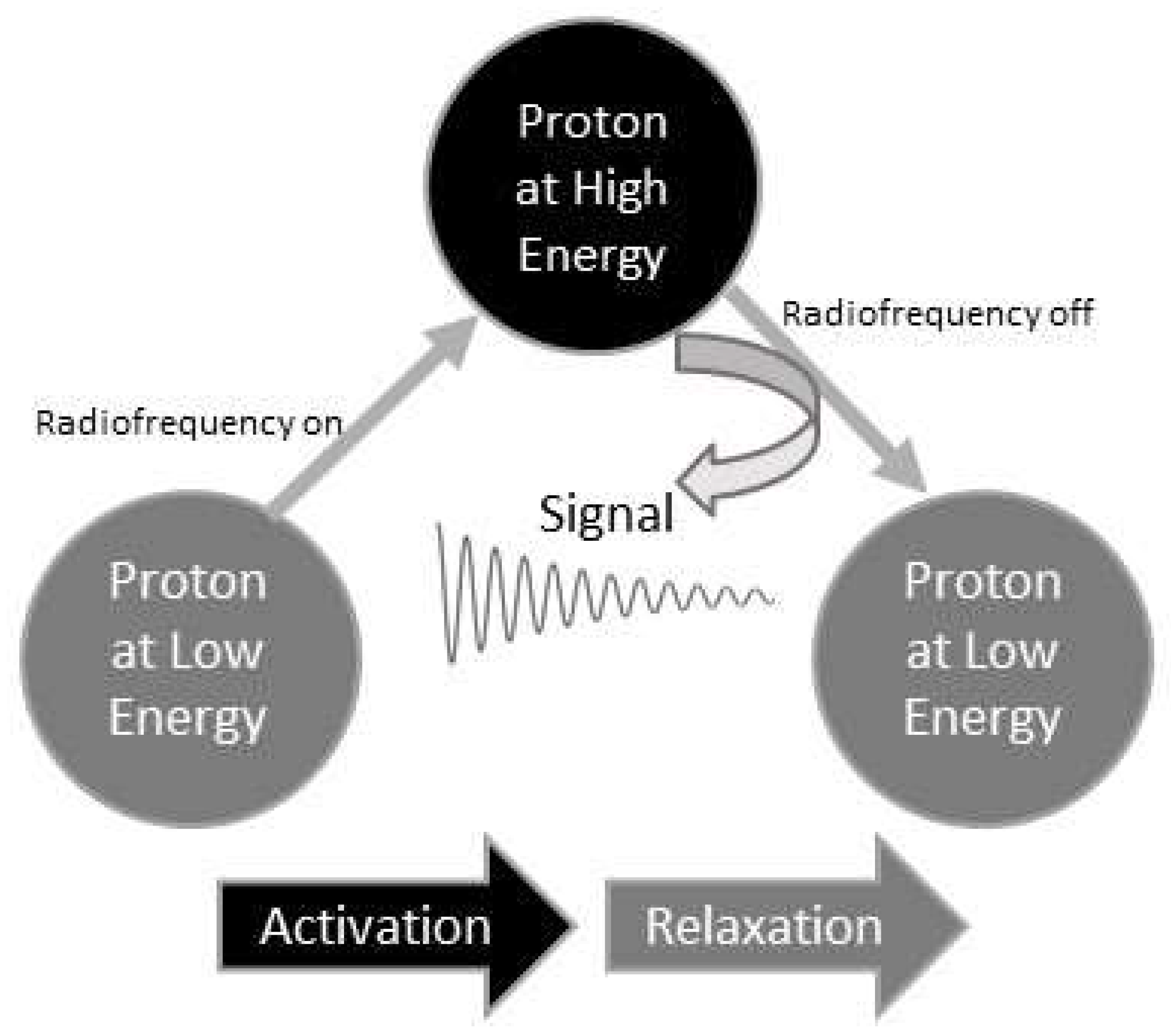
After the radiofrequency pulses are turned off, the nuclei undergo relaxation, releasing the absorbed energy and returning to their original energy levels. The decaying signal resulting from this relaxation process is captured by a receiver coil surrounding the sample tube. The weak energy-varying currents induced by the relaxation are detected as raw signals from the molecules.
Figure 1 uses a proton as an example nucleus to illustrate how a proton signal is generated.
Before becoming raw NMR data, these signals undergo amplification and digitization. Raw NMR data visually portray signal changes over time, as seen in
Figure 1’s middle section, capturing their dynamic variations. Hence, they are termed time domain NMR data.
NMR Data Pre-processing
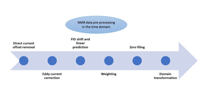
NMR signals recorded in the time domain cannot be directly used for clinical and research purposes. Various pre-processing steps are necessary to transform the raw NMR data into a suitable format for analysis.
The initial step in NMR data pre-processing is the conversion of raw NMR time-domain files, referred to as Free Induction Decay (FID) data, from an unreadable binary format to text. This conversion is a standard and uncomplicated task that is typically carried out by NMR software, including the ones listed in
Table 1. The resulting text file represents the data in a way that makes it readable and usable.
The second pre-processing step removes unwanted signal interference known as “’Direct Current (DC) offsets,” which can affect FID signals. Tools like TopSpin, SpinWorks, NMRPipe, and rNMR (
Table 1) perform this task to restore signal integrity for analysis.
The third step involves fixing "Eddy Current" (EC) effects. Eddy currents are like swirling currents caused by the radiofrequency turning on and off or the presence of nearby metal objects, among other things. These swirling currents can disrupt the magnetic field of the NMR machine and make our data a bit messy. Correcting for EC effects is a complex task that involves compensating for these distortions. Specialized tools designed for MRI data, such as the "eddy" tool listed in
Table 1, are often used for this purpose.
The fourth pre-processing step involves FID shift and Linear Prediction (LP). FID shift aligns the FID signal by shifting data points left or right when there is time misalignment. Linear Prediction (LP) estimates missing values caused by short data recordings or FID shift. Commonly used tools for FID shift and LP, listed in
Table 1, include TopSpin, SpinWorks, ACD/LABS, NMRPipe, and Mnova.
The fifth pre-processing step is weighting, often used to adjust signal decay in the time domain. This involves multiplying the time-domain data by a chosen nonlinear weighting function, which can make the signal decay faster or slower. The software tools listed in
Table 1 are capable of handling this step during NMR data pre-processing.
The sixth step, zero filling, involves adding zeros to the end of the FID to improve apparent time resolution. While these additional data points don’t provide new information about the signal, they enhance its visual representation and can benefit specific data analysis techniques. All the software tools in
Table 1 can perform zero filling.
The final pre-processing step in the time domain is transformation, which involves converting the time-domain FID data into a different domain using a mathematical operation. This transformation is supported by all the software tools listed in
Table 1.
These pre-processing steps are essential for effectively analysing NMR time domain data. While some recent reviews may have omitted some of these steps 23–26, our review article aims to comprehensively examine each pre-processing step, focusing on the rationale, algorithms, and statistical aspects. We skip converting FID data from binary to text because that’s a basic computer science task. Instead, we concentrate on the theory and the proper application of the subsequent steps.
Direct current (DC) offset removal
To ensure accurate NMR data analysis, we need to address Direct Current (DC) offset, a constant voltage added to the NMR signal due to various factors like instrument imperfections or interference.
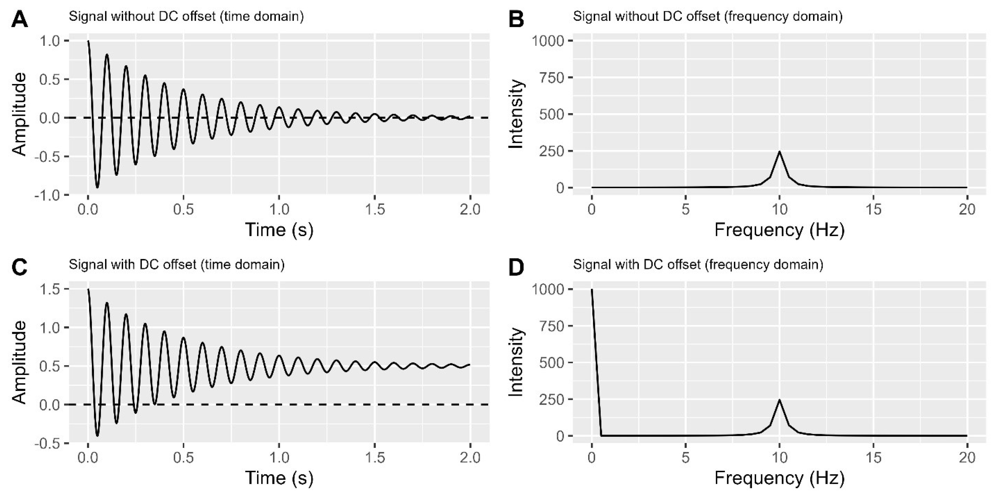
Before delving into DC offsets, let’s simplify a crucial concept: frequency. Frequency measures how quickly a signal changes, in Hertz (Hz), representing cycles per second. In
Figure 2A, the signal centres at zero and completes 10 cycles per second (10 Hz). To distinguish signals, we convert time domain data into the frequency domain, where signals are represented based on their frequencies.
Figure 2B shows a peak at 10 Hz.
However, when a signal detector in an NMR spectrometer has a DC voltage offset, the signal’s centre shifts away from zero in the time domain plot (
Figure 2C), causing an unexpected non-signal line on the very left in the frequency domain plot (
Figure 2D). To address this issue, it is necessary to remove the DC offset in the time domain. Currently, there are at least three methods available to accomplish this task.
Last data point method
Subtract the last data point’s value from all data points using this formula: "new data point" = "original data point" - "last data point." It’s simple but not very reliable when signals haven’t converged.
Tail points method
Average the last 10-20% of data points and subtract this average from all data points using the formula: "new data point" = "original data point" - "average of tail points." This method is generally more reliable than the last point 27. However, it’s less effective and might even perform worse than the last point method when dealing with signal asymmetry or insufficient recording time.
Phase cycling method
Before discuss this method, let’s describe what is phase. Phase indicates position within a cycle in a signal and it causes a signal upon and down as shown in
Figure 2A. Mathematically, a signal in
Figure 2A contains a cosine function, and the angle of this cosine function is phase.
Refer to
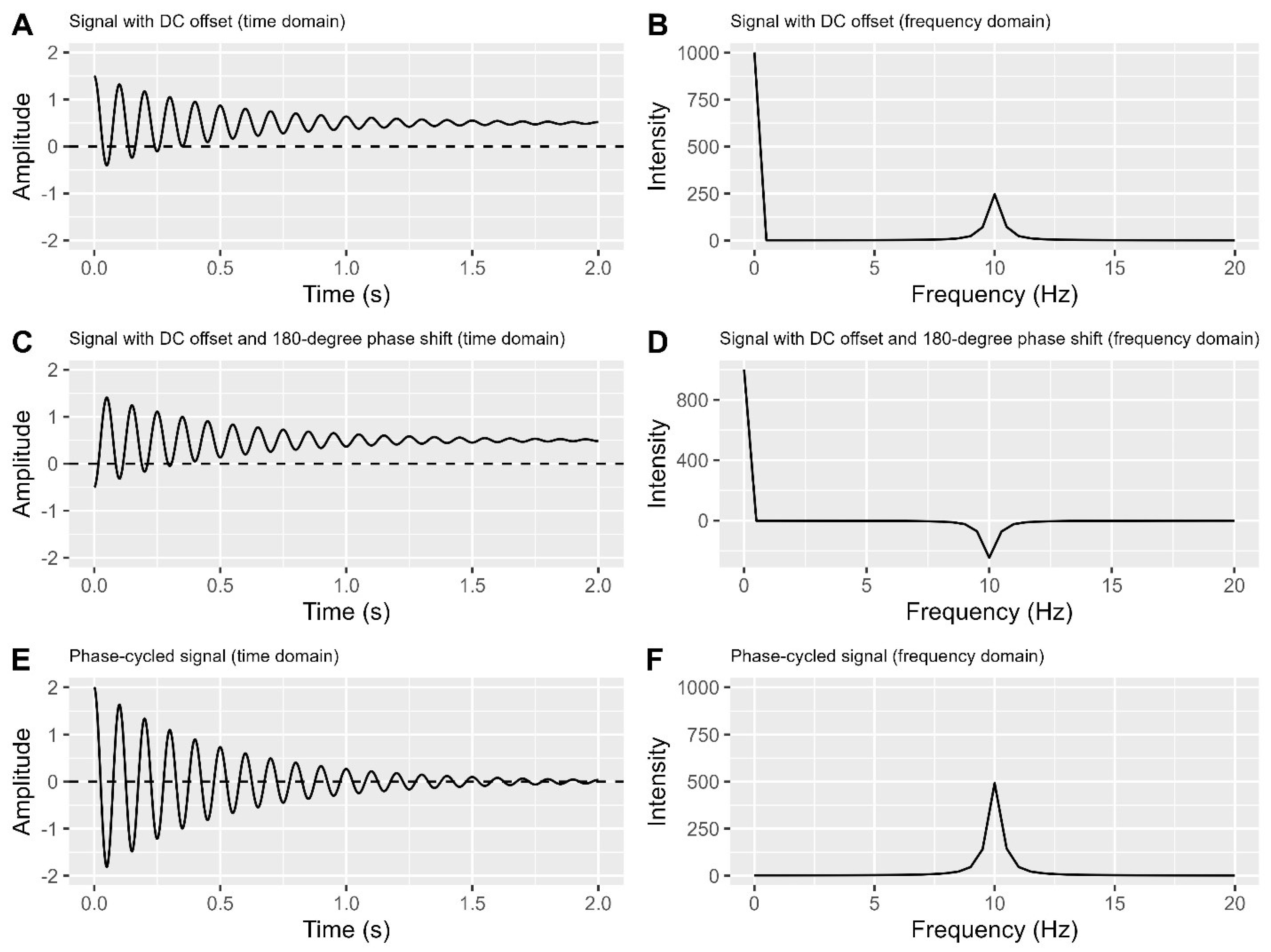
Figure 3 to understand phase cycling method. In
Figure 3A-B, we see a signal with a DC offset in both time and frequency domains, similar to
Figure 2C-D. Without shifting the centreline (0.5 in
Figure 3A), flip the signal around it, creating a mirror image (
Figure 3C) with a 180-degree phase difference from the original (
Figure 3A), this is equivalent to add 180 degrees of phase into cosine function at each time point. Transforming
Figure 3C into
Figure 3D provides frequency domain data with a reversed signal peak direction. Notably, the DC offset remains consistent in
Figure 3A,C, and the unexpected line observed in
Figure 3B also appears in
Figure 3D.
Subtracting
Figure 3A from
Figure 3C in
Figure 3E cleans the signal by eliminating DC offset and doubling its strength (maximum amplitude when DC offset is absent). Transforming
Figure 3E into
Figure 3F maintains this doubled signal strength, representing the peak area under the curve in the time domain, and eliminates the unexpected line.
Real NMR data contain multiple signals, a simple flip does not work, we need another detector to record signals with 180-degrees apart. Then we can apply the same subtraction to obtain clean signals without DC offset, but be aware that the signal amounts are doubled.
Comment: The most reliable approach to handle DC offset is by phase cycling when an extra detector is available. In cases where the FID recording time is sufficiently long, estimating the DC offset using either the last data point or the tail points can be considered. Unfortunately, there is no optimal solution for handling DC offset in other situations.
Eddy current (EC) correction
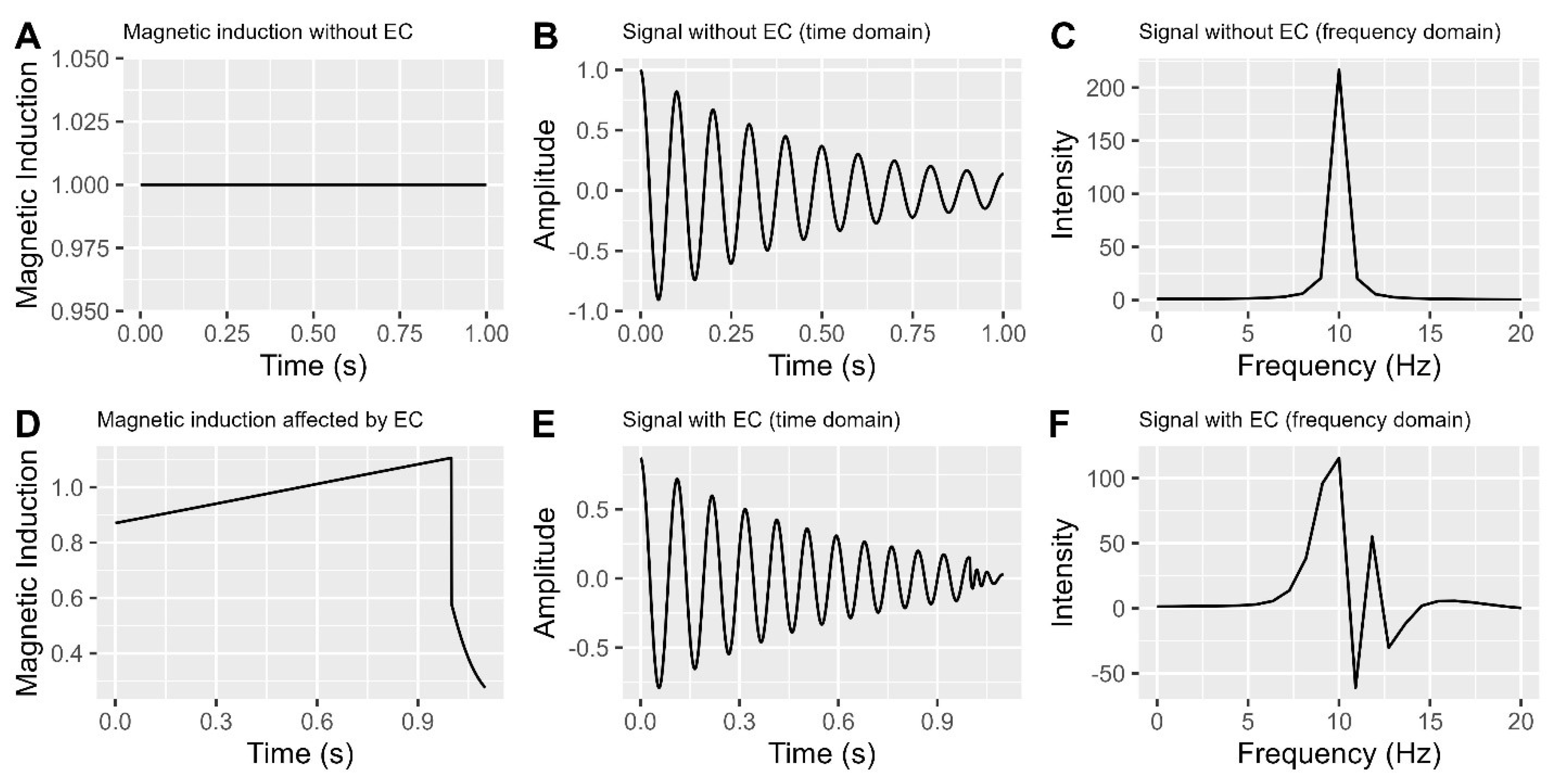
Eddy currents cause distortions in the NMR magnetic field, leading to the following effects: variations in observed frequencies, fluctuations in signal amplitude, and phase distortions in acquired NMR signals.
A. Magnetic induction without eddy currents.
B. NMR signal without eddy currents (Time domain).
C. NMR signal without eddy currents (Frequency domain).
D. Magnetic induction affected by eddy currents.
E. NMR signal with eddy currents (Time domain).
F. NMR signal with eddy currents (Frequency domain).
In
Figure 4A, when there are no eddy currents, a constant magnetic induction results in a consistent cyclic signal in the time domain (
Figure 4B) and a single symmetric peak in the frequency domain (
Figure 4C). However, the presence of eddy currents (as seen in
Figure 4D) causes the time domain signal to become irregular (
Figure 4E) and introduces multiple peaks, including negative ones, in the frequency domain (
Figure 4F).
Figure 4F illustrates significant signal distortion caused by eddy currents, resulting in changes in peak heights and areas under curves used for data analysis. To ensure accurate data interpretation and analysis, it is crucial to correct these distortions.
Eddy current correction aims to remove the effects of eddy currents (EC). We’ll discuss three NMR methods and one MRI method for addressing them.
Phase correction with reference FID
This method addresses phase distortions caused by eddy currents (EC) through the use of an additional FID file containing only a reference signal. By subtracting the reference FID’s phase vector from that of the experimental FID, we obtain an EC-corrected phase vector. Using these corrected phases, we recalculate the EC-corrected FID 28.
This approach assumes consistent acquisition settings for both the experimental and reference FIDs, ensuring identical phase errors due to EC. While this method could effectively remove most EC effects, it does result in the loss of the reference signal. In addition, it’s important to be aware that this procedure may not fully correct all frequency shifts caused by EC, which could still influence peak positions in the frequency domain.
Removal of solvent signal
Eddy currents mainly affect the strongest signal. To counter this, we choose a solvent signal with a significantly different frequency and significantly increase its concentration in the sample. This allows us to exclude or ignore the solvent signal range in the frequency domain, reducing the impact of eddy currents. While this approach typically minimizes eddy current effects 28, it may not work well if signals of interest share frequencies with the solvent signals, as eddy currents can affect signals beyond the strongest one.
Phase error correction with opposite induction directions
To address phase errors caused by eddy currents, we employ a two-step approach. Initially, we apply a positive magnetic induction as shown in
Figure 4A, followed by a repeat with a negative induction, keeping all other parameters constant. In the second step, the phase error direction reverses while maintaining similar magnitudes. Adding the time domain signals from both steps effectively cancels out the eddy current-induced phase errors
28,29. It’s important to note that this method mitigates uneven phase errors, while some residual frequency shifts may remain. Additionally, this method doubles the remaining signal strength. To return to the original signal strength, we need to divide FID by 2.
EC-induced magnetic model
The Eddy Current (EC)-induced magnetic field model primarily applies to MRI rather than basic NMR data. This model establishes the relationship between the EC-induced magnetic field and spatial coordinates, with options for handling non-linear effects.
As we can’t directly measure the EC-induced magnetic field, we rely on an iterative optimization process to determine model parameters. Specialized software like "eddy" 22,30 plays a crucial role in this process. Once we obtain these model parameters and estimate the EC-induced magnetic induction, we can correct MRI data for EC effects.
Comment: Eddy current issues can lead to significant alterations in NMR data. While some argue that this concern has diminished with improved NMR instruments 28, it is not advisable to assume the absence of eddy current problems and overlook the step of EC correction. We recommend the following procedure:
- 1)
Check the time and frequency domains for eddy current issues, focusing on distorted peaks (see
Figure 4F).
- 2)
If you detect eddy current effects and have the necessary resources, perform EC correction in the time domain.
- 3)
If resources are limited, address the issue during domain transformation. Prioritize phase error correction and chemical shift calibration during frequency domain pre-processing.
FID shift and linear prediction
FID shift
FID shift involves shifting data points in the FID either to the left or to the right by a certain number of points. A left shift moves some points before time 0 beyond the FID, while a right shift delays the FID and leaves some points as NAs or zeros.
Both left and right shifts address the issue of distortion at the starting points of the FID. A left shift is suitable for fully recorded FIDs, especially when the shift is small, while a right shift is used for intentionally delayed recordings and should be followed by linear prediction (LP).
The starting part of the FID is crucial as it directly influences the signal areas in the frequency domain. Without compensation, an FID shift decreases the starting point’s amplitude and affects the signal’s area, leading to systematic measurement errors on signal strength.
Linear prediction (LP)
Linear prediction (LP) is a common technique used to recover lost data resulting from FID shifts or intentional recording delays. LP estimates missing data through either backward or forward prediction.
Backward LP fills in the initial part of the FID by estimating it from neighbouring points immediately following the missing data.
Forward LP, on the other hand, extends the FID’s tail or fills in missing values at the end. It accomplishes this by predicting these less informative points using a linear combination of more informative points from the leading part. This makes forward LP more accurate than backward LP in many cases.
Here are the LP formulas
31:
In these formulas, m represents the base point index, P is the total number of base points, is the predicted point, and are the base points used for backward and forward LP, respectively. stands for the coefficient of a base point, and is the random error associated with the predicted point. The prediction process involves an iterative optimization process that utilizes a loss function, such as squared differences between and .
Comment: Care is needed when applying FID shift and backward LP, as they can introduce problems such as phase errors, distortion, and unrecoverable errors in the data 32. FID shifts, whether left or right, can result in phase errors. Generally, a small left shift is safer than a larger right shift that often requires backward LP.
In contrast, forward LP is generally considered safer, as long as the percentage of predicted data remains reasonable.
Weighting
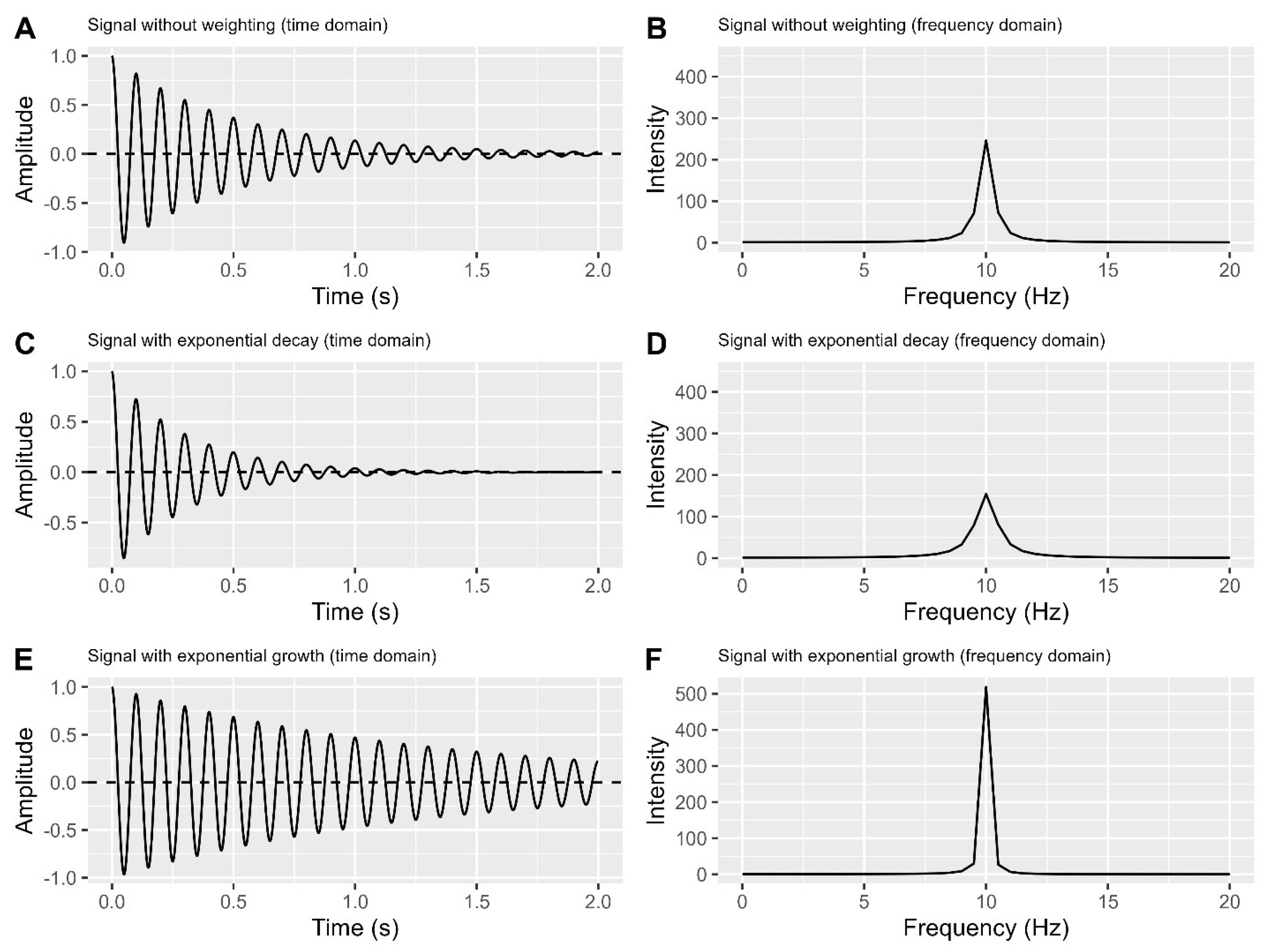
Weighting involves multiplying the FID with a nonlinear weighting function, such as exponential, Gaussian, or sine bell functions, with the aim of enhancing sensitivity or resolution 33. This practice is widely utilized in current methodologies 9,34–39.
Figure 5A-B shows a simulated FID in the time and frequency domains. Applying a nonlinear decreasing weighting function, like a decreasing exponential decay, significantly attenuates the FID’s tail while sparing the starting part (
Figure 5C). This process can reduce the ending part to zeros, which is referred to as apodization
40.
The decreasing weighting function enhances the signal-to-noise ratio (SNR) by reducing noise but may broaden peaks in the frequency domain (
Figure 5D). This broadening reduces resolution and may cause peak overlap, making area estimation more challenging
10,40.
A. Time domain plot of a simulated FID with a single peak.
B. Frequency domain plot corresponding to A.
C. Time domain plot of A times an exponential decay (). Here, j is index of a given point, and N is the total number of data points in FID.
D. Frequency domain plot corresponding to C.
E. Time domain plot of A times an exponential growth ().
F. Frequency domain plot corresponding to E.
On the other hand, applying a nonlinear, uneven rising function like a rising exponential enhances FID resolution (
Figure 5E) and produces a narrow peak in the frequency domain (
Figure 5F). However, it increases noise in the FID tail, reducing SNR and potentially introducing distorted and asymmetric peaks
41.
Comment: Using weighting functions presents a dilemma. While they can improve sensitivity or resolution, achieving both simultaneously is impossible. Additionally, weighting functions have the potential to distort data, making recovery difficult. We recommend caution when applying weighting functions unless there’s a clear understanding of the data and a specific goal to enhance sensitivity or resolution. If used, ensure consistent application within the same experiment, as
Figure 5 demonstrates the potential for data incomparability otherwise.
Zero Filling
Zero filling is a common technique to increase the number of data points in a discrete Fourier transform (DFT) of a signal. It involves adding zeros to the end of the time-domain signal before performing the DFT. This expands the number of points in the DFT and the frequency bins in the frequency domain, creating the illusion of higher digital resolution 27.
However, this increased resolution is artificial and doesn’t provide additional information about the signal. It can also amplify noise due to the added zeros.
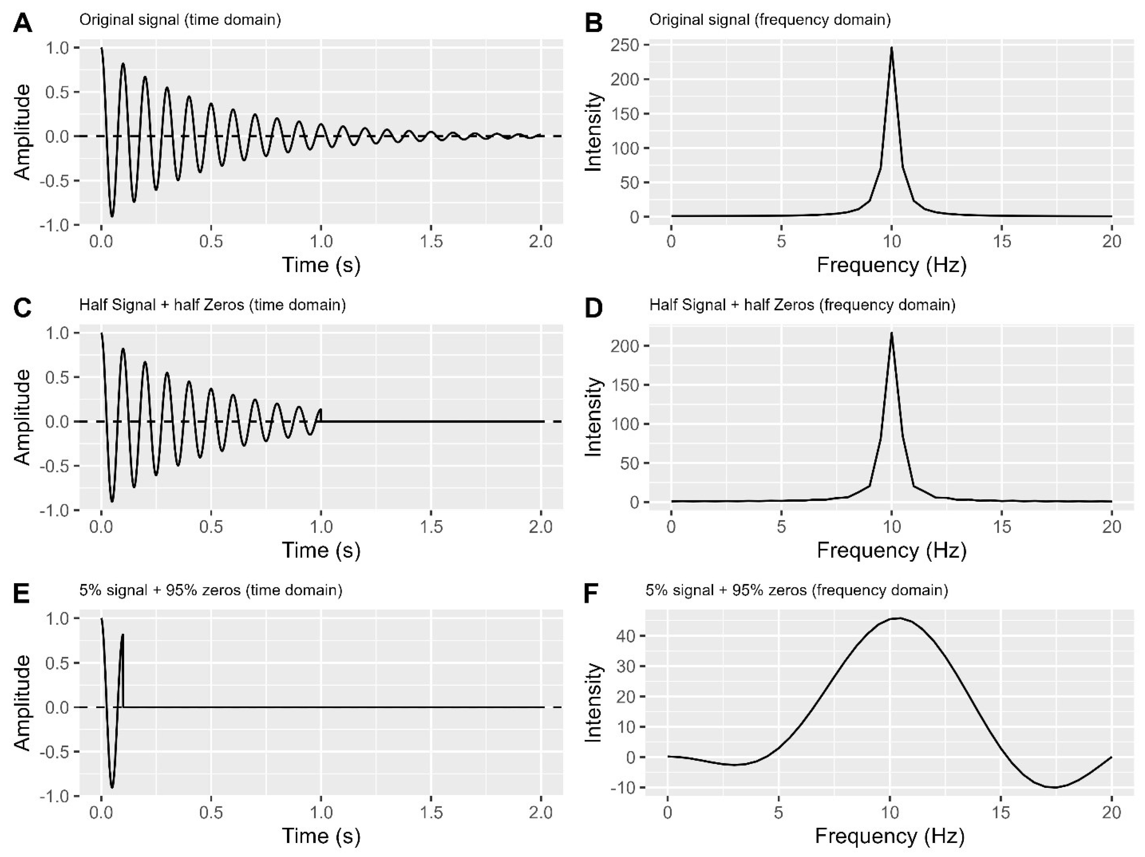
When applying zero filling, it is advisable to ensure that the endpoints of the FID are already close to zero. Compared to original signal (
Figure 6A-B), even though only half of the signal points are used in
Figure 6C, the endpoint of this half signal is close to zero. As a result, the signal in the frequency domain (
Figure 6D) does not differ significantly from the original signal peak (
Figure 6B).
A. Original signal in the time domain.
B. Frequency domain plot of the original signal.
C. Half signal + half zeros in the time domain.
D. Frequency domain plot of the half signal + half zeros.
E. 5% signal + 95% zeros in the time domain.
F. Frequency domain plot of the 5% signal + 95% zeros.
Failure to meet this condition can result in wiggles or distorted peaks (
Figure 6E-F). Methods like forward linear prediction and apodization decay functions
27 can help in such cases, but their effectiveness may vary.
Comment: Zero filling is generally safe when adequate data is recorded and FID endpoints are near zero. However, in cases with very few data points (
Figure 6E-F), it may not offer significant benefits. It’s better to extend recording time for more observed data points before considering zero filling. If you apply zero filling, ensure the same number of zeros is used for all FIDs within a single experiment to maintain data comparability.
Domain Transformation
Domain transformation is a crucial step in which the time domain data of FID is converted into the frequency domain. This transformation is necessary because most subsequent data analyses are performed in the frequency domain.
The primary method for domain transformation is the discrete Fourier transform (DFT). It mathematically analyses the frequency content of a discrete signal, turning each FID signal into a single peak in the resulting spectrum 40.
The DFT formula can be broken down as follows:
represents the kth complex number in the frequency domain.
represents the nth complex number in the time domain.
N is the total number of data points in the sequence.
k is the frequency bin index, ranging from 0 to N-1.
To compute , each data point is multiplied by a complex exponential term and the contributions are summed up for all n values. This process calculates the contribution of each data point at different frequencies and combines them to form the frequency domain representation.
Another approach is the linear model, which can be used independently or complementarily with the Fourier Transform 42. However, for FIDs with multiple signals, the linear model alone may be less accurate than the Fourier transform.
The Bayesian approach is a third method 43,44, offering potential improvements in domain transformation. However, its performance relies on prior distribution information.
The fourth method is the wavelet transform 45, which is less commonly used but advantageous for handling uneven frequencies. Unlike the Fourier transform, which assumes constant frequencies, the wavelet transform can handle uneven frequency data, making it useful for FIDs affected by eddy currents (as discussed in section "
Eddy Current (EC) Correction").
Comment: For standard cases without eddy current issues, we recommend using the Fourier transform alone. It’s a reliable method that doesn’t rely on prior knowledge or the number of signals. However, when eddy current problems are present and haven’t been corrected, we suggest using the wavelet transform instead of the Fourier transform. Eddy currents can alter signal frequencies, which Fourier transform alone can’t address. The wavelet transform is suitable for handling FIDs affected by eddy currents without needing additional data 46. Note that after wavelet transform, frequency domain peaks may not be perfectly sharp or symmetric, but forcing them into a predetermined shape can lead to information loss.
Conclusion/Discussion
NMR and its variants play crucial roles in research and clinical settings. In this article, we’ve delved into the mathematical and statistical aspects of common pre-processing steps, shedding light on their challenges and algorithmic choices.
In previous sections, we’ve covered six essential time domain pre-processing steps. While our review follows the typical pre-processing sequence, it’s worth noting that forward LP can be used to extend the tail before DC correction and zero filling, especially when the recorded FID is too short.
Table 2 provides a summary of the discussions in previous sections, including additional steps for applying LP. We would like to emphasize some key points from the table.
- 1)
DC Offset Correction: Prioritize investigating, estimating, and removing DC offsets. This can usually be done with phase cycling or a sufficiently long FID recording.
- 2)
Eddy Current (EC) Correction: EC-induced distortion is a challenging pre-processing step. Investigate EC issues in both time and frequency domains. If specific conditions are met, EC correction is feasible. Otherwise, use wavelet transform instead of FT during domain transformation to address EC-affected signals.
- 3)
FID Shift: In general, avoid FID shifts that result in information loss. Exceptions include intentional pre-acquisition delays for severe distortion, followed by backward LP. Forward LP is useful for extending the FID tail to enhance digital resolution, either on its own or before DC offset removal and zero filling.
- 4)
Weighting: Weighing can enhance sensitivity or resolution, but not both at once. Only apply weighting if you’re confident it’s necessary, and use the same function for all spectra within an experiment to ensure comparability.
- 5)
Zero Filling: Zero filling can boost digital FID resolution. It’s recommended if the ending FID values are close to zero. If not, consider applying forward LP before zero filling, provided DC offset is not an issue.
- 6)
Domain Transformation: FT is the primary method for domain transformation and works well in most cases. However, for uncorrected EC effects, wavelet transform is a better alternative. While many NMR pre-processing software tools lack wavelet transform options, dedicated packages in languages like R and Python can perform this technique.
Table 2.
Summary of reviewed NMR time domain pre-processing steps.
Table 2.
Summary of reviewed NMR time domain pre-processing steps.
| Pre-processing step |
Possible problems |
Our recommendations |
| DC (Direct Current) offset removal |
The DC offset might not be correctly estimated |
Approach with two sets of scans is the best method. When this is not practical, we need a converged tail of FID to estimate DC offset and remove it. When recording time is too short, forward LP might be applied before DC offset estimation. |
| EC (Eddy Current) correction |
Additional data or specific adjustments might not be available. |
Reference FID, isolated solvent peak, and opposite magnetic inductions are especially useful to remove EC. When extra data and tools are not available, skip this step and take care of the problem in domain transformation. |
| FID shift and LP (Linear Prediction) |
Might cause severe phasing problems, distortion and unrecoverable errors in FID data. |
FID shift plus backward LP is useful to deal with serious distortion in the leading part of FID even though the process is still risky. Otherwise, we suggest no FID shift. But forward LP to extend tail is recommended when the data are recorded too short. |
| Weighting |
Could distort data that cannot be recovered later. |
Skip this step unless you know data very well and you are sure to improve sensitivity or to enhance resolution. |
| Zero filling |
Too many zero additions might change true information. |
Zero filling is generally recommended, but it is important to ensure that the ending values are already close to zero and that too many zeros are not added. Otherwise, forward LP is needed before zero filling. |
| Domain transformation |
When prior knowledge is not available, and if there are many peaks in the FID, some methods might not work. |
In general, FT is the best choice since it does not require additional information and it works well for multiple signals. However, wavelet transform is a better choice when an EC problem exists. |
In addition to specific pre-processing discussions, it’s crucial to respect the data and minimize unnecessary alterations. Preserving the original data integrity is essential. Instead of excessive manipulation, consider modelling noise during subsequent statistical analysis. This approach maintains the accuracy and reliability of data interpretation while minimizing unintended distortion.
References
- Bertholdo, D.; Watcharakorn, A.; Castillo, M. Brain Proton Magnetic Resonance Spectroscopy: Introduction and Overview. Neuroimaging Clin N Am 2013, 23, 359–380. [Google Scholar] [CrossRef] [PubMed]
- Barajas, R. F. J.; Politi, L. S.; Anzalone, N.; Schöder, H.; Fox, C. P.; Boxerman, J. L.; Kaufmann, T. J.; Quarles, C. C.; Ellingson, B. M.; Auer, D.; Andronesi, O. C.; Ferreri, A. J. M.; Mrugala, M. M.; Grommes, C.; Neuwelt, E. A.; Ambady, P.; Rubenstein, J. L.; Illerhaus, G.; Nagane, M.; Batchelor, T. T.; Hu, L. S. Consensus Recommendations for MRI and PET Imaging of Primary Central Nervous System Lymphoma: Guideline Statement from the International Primary CNS Lymphoma Collaborative Group (IPCG). Neuro Oncol 2021. [Google Scholar] [CrossRef] [PubMed]
- Sorger, B.; Goebel, R. Real-Time FMRI for Brain-Computer Interfacing. Handb Clin Neurol 2020, 168, 289–302. [Google Scholar] [CrossRef] [PubMed]
- Liu, S.; Xiong, Y.; Dai, E.; Zhang, J.; Guo, H. Improving Distortion Correction for Isotropic High-Resolution 3D Diffusion MRI by Optimizing Jacobian Modulation. Magn Reson Med 2021. [Google Scholar] [CrossRef] [PubMed]
- Li, H.; Zhang, Q.; Duan, Q.; Jin, J.; Hu, F.; Dang, J.; Zhang, M. Brainstem Involvement in Amyotrophic Lateral Sclerosis: A Combined Structural and Diffusion Tensor MRI Analysis. Front Neurosci 2021, 15, 675444. [Google Scholar] [CrossRef] [PubMed]
- Patra, A.; Bera, M. Spectroscopic Investigation of New Water Soluble MnII2 and MgII2 Complexes for the Substrate Binding Models of Xylose/Glucose Isomerases. Carbohydrate Research 2014, 384, 87–98. [Google Scholar] [CrossRef]
- Smolinska, A.; Blanchet, L.; Buydens, L. M. C.; Wijmenga, S. S. NMR and Pattern Recognition Methods in Metabolomics: From Data Acquisition to Biomarker Discovery: A Review. Analytica Chimica Acta 2012, 750, 82–97. [Google Scholar] [CrossRef]
- Ferry-Dumazet, H.; Gil, L.; Deborde, C.; Moing, A.; Bernillon, S.; Rolin, D.; Nikolski, M.; de Daruvar, A.; Jacob, D. MeRy-B: A Web Knowledgebase for the Storage, Visualization, Analysis and Annotation of Plant NMR Metabolomic Profiles. BMC Plant Biology 2011, 11, 104. [Google Scholar] [CrossRef]
- Cuperlovic-Culf, M.; Cormier, K.; Touaibia, M.; Reyjal, J.; Robichaud, S.; Belbraouet, M.; Turcotte, S. (1)H NMR Metabolomics Analysis of Renal Cell Carcinoma Cells: Effect of VHL Inactivation on Metabolism. Int J Cancer 2016, 138, 2439–2449. [Google Scholar] [CrossRef]
- Ebbels, T. M. D.; De Iorio, M. Statistical Data Analysis in Metabolomics. In Handbook of Statistical Systems Biology; John Wiley & Sons, Ltd, 2011; pp 163–180. [CrossRef]
- Brzezinska, J.; Gdaniec, Z.; Popenda, L.; Markiewicz, W. T. Polyaminooligonucleotide: NMR Structure of Duplex DNA Containing a Nucleoside with Spermine Residue, N-[4,9,13-Triazatridecan-1-Yl]-2′-Deoxycytidine. Biochimica et Biophysica Acta (BBA) - General Subjects 2014, 1840, 1163–1170. [Google Scholar] [CrossRef] [PubMed]
- Bonneau, E.; Legault, P. NMR Localization of Divalent Cations at the Active Site of the Neurospora VS Ribozyme Provides Insights into RNA-Metal-Ion Interactions. Biochemistry 2014, 53, 579–590. [Google Scholar] [CrossRef] [PubMed]
- Lu, G. J.; Opella, S. J. Resonance Assignments of a Membrane Protein in Phospholipid Bilayers by Combining Multiple Strategies of Oriented Sample Solid-State NMR. J Biomol NMR 2014, 58, 69–81. [Google Scholar] [CrossRef] [PubMed]
- Smith, E. A. Advanced Techniques in Pediatric Abdominopelvic Oncologic Magnetic Resonance Imaging. Magnetic resonance imaging clinics of North America 2013, 21, 829–841. [Google Scholar] [CrossRef] [PubMed]
-
TopSpin | NMR Data Analysis | Bruker. https://www.bruker.com/en/products-and-solutions/mr/nmr-software/topspin.html (accessed on 22 June 2021).
-
NMR Webpage - SpinWorks. https://home.cc.umanitoba.ca/~wolowiec/spinworks/ (accessed on 22 June 2021).
-
Chemistry Software for Analytical and Chemical Knowledge Management. https://www.acdlabs.com/ (accessed on 22 June 2021).
-
NMRPipe. https://spin.niddk.nih.gov/bax/software/NMRPipe/NMRPipe.html (accessed on 22 June 2021).
-
rNMR: Open Source Software for NMR Data Analysis. http://rnmr.nmrfam.wisc.edu/ (accessed on 22 June 2021).
- mestrelab. Mnova. Mestrelab. https://mestrelab.com/software/mnova/ (accessed on 22 June 2021).
-
Chenomx Inc | Metabolite Discovery and Measurement. https://www.chenomx.com/ (accessed on 22 June 2021).
-
eddy - FslWiki. https://fsl.fmrib.ox.ac.uk/fsl/fslwiki/eddy (accessed on 22 June 2021).
- Pathmasiri, W.; Kay, K.; McRitchie, S.; Sumner, S. Analysis of NMR Metabolomics Data. In Computational Methods and Data Analysis for Metabolomics; Li, S., Ed.; Springer US: New York, NY, 2020; pp. 61–97. [Google Scholar] [CrossRef]
- Cambiaghi, A.; Ferrario, M.; Masseroli, M. Analysis of Metabolomic Data: Tools, Current Strategies and Future Challenges for Omics Data Integration. Briefings in bioinformatics 2017, 18, 498–510. [Google Scholar] [CrossRef]
- Staniszewski, M.; Skorupa, A.; Boguszewicz, L.; Sokol, M.; Polanski, A. Preprocessing Methods in Nuclear Magnetic Resonance Spectroscopy. In Information Technologies in Medicine: 5th International Conference, ITIB 2016 Kamień Śląski, Poland, June 20 - 22, 2016 Proceedings, Volume 1; Piętka, E., Badura, P., Kawa, J., Wieclawek, W., Eds.; Springer International Publishing: Cham, 2016; pp. 341–352. [Google Scholar] [CrossRef]
- Mohamed, A.; Nguyen, C. H.; Mamitsuka, H. Current Status and Prospects of Computational Resources for Natural Product Dereplication: A Review. Briefings in Bioinformatics 2015, 17, 309–321. [Google Scholar] [CrossRef] [PubMed]
- Rule, G. S.; Hitchens, T. K. Fundamentals of Protein NMR Spectroscopy. 2006.
- Jiru, F. Introduction to Post-Processing Techniques. Eur J Radiol 2008, 67, 202–217. [Google Scholar] [CrossRef] [PubMed]
- Bieri, O.; Markl, M.; Scheffler, K. Analysis and Compensation of Eddy Currents in Balanced SSFP. Magnetic Resonance in Medicine 2005, 54, 129–137. [Google Scholar] [CrossRef]
- Andersson, J. L. R.; Sotiropoulos, S. N. An Integrated Approach to Correction for Off-Resonance Effects and Subject Movement in Diffusion MR Imaging. NeuroImage 1, 125, 1063–1078. [CrossRef]
- Feng, H.; Cai, S.; Chen, Z.; Lin, M.; Feng, J. Application of the Forward Linear Prediction on High-Resolution NMR Spectra in Inhomogeneous Fields. Spectrochim Acta A Mol Biomol Spectrosc 2008, 71, 1027–1031. [Google Scholar] [CrossRef]
- Lindon, J. Peter Bigler NMR Spectroscopy: Processing Strategies, 2nd Edn Wiley-VCH, Weinheim, 1999, Pp Xi+253 plus CD-ROM, £95.00. NBM NMR in Biomedicine 2000, 13, 312–313. [Google Scholar] [CrossRef]
- Atta-ur-Rahman; Choudhary, M. I. CHAPTER 1 - The Basics of Modern NMR Spectroscopy. In Solving Problems with NMR Spectroscopy; Atta-ur-Rahman, Choudhary, M. I., Eds.; Academic Press: San Diego, 1996; pp 1–89. [CrossRef]
- Betson, T. R.; Augusti, A.; Schleucher, J. Quantification of Deuterium Isotopomers of Tree-Ring Cellulose Using Nuclear Magnetic Resonance. Anal. Chem. 2006, 78, 8406–8411. [Google Scholar] [CrossRef]
- Croitor-Sava, A.; Beck, V.; Sandaite, I.; Van Huffel, S.; Dresselaers, T.; Claus, F.; Himmelreich, U.; Deprest, J. High-Resolution 1H NMR Spectroscopy Discriminates Amniotic Fluid of Fetuses with Congenital Diaphragmatic Hernia from Healthy Controls. J. Proteome Res. 2015, 14, 4502–4510. [Google Scholar] [CrossRef]
- Beckmann, N. In Vivo MR Techniques in Drug Discovery and Development; Taylor & Francis: New York, 2006. [Google Scholar]
- Luck, M.; Le Moyec, L.; Barrey, E.; Triba, M.; Bouchemal, N.; SAVARIN, P.; ROBERT, C. Energetics of Endurance Exercise in Young Horses Determined by Nuclear Magnetic Resonance Metabolomics. Frontiers in Physiology 2015, 6, 198. [Google Scholar] [CrossRef] [PubMed]
- Motegi, H.; Tsuboi, Y.; Saga, A.; Kagami, T.; Inoue, M.; Toki, H.; Minowa, O.; Noda, T.; Kikuchi, J. Identification of Reliable Components in Multivariate Curve Resolution-Alternating Least Squares (MCR-ALS): A Data-Driven Approach across Metabolic Processes. Sci Rep 2015, 5, 15710–15710. [Google Scholar] [CrossRef] [PubMed]
- del Campo, G.; Zuriarrain, J.; Zuriarrain, A.; Berregi, I. Quantitative Determination of Carboxylic Acids, Amino Acids, Carbohydrates, Ethanol and Hydroxymethylfurfural in Honey by (1)H NMR. Food Chem 2016, 196, 1031–1039. [Google Scholar] [CrossRef] [PubMed]
- Ebbels, T. M. D.; Lindon, J. C.; Coen, M. Processing and Modeling of Nuclear Magnetic Resonance (NMR) Metabolic Profiles. Methods Mol Biol 2011, 708, 365–388. [Google Scholar] [CrossRef]
- Van Horn, W. D.; Beel, A. J.; Kang, C.; Sanders, C. R. The Impact of Window Functions on NMR-Based Paramagnetic Relaxation Enhancement Measurements in Membrane Proteins. Biochim Biophys Acta 2010, 1798, 140–149. [Google Scholar] [CrossRef]
- Koehl, P. Linear Prediction Spectral Analysis of NMR Data. Progress in Nuclear Magnetic Resonance Spectroscopy 1999, 34, 257–299. [Google Scholar] [CrossRef]
- Bretthorst, G. L. Bayesian Analysis. V. Amplitude Estimation for Multiple Well-Separated Sinusoids. JMRES Journal of Magnetic Resonance (1969) 1992, 98, 501–523. [Google Scholar] [CrossRef]
- Krishnamurthy, K. CRAFT (Complete Reduction to Amplitude Frequency Table)--Robust and Time-Efficient Bayesian Approach for Quantitative Mixture Analysis by NMR. Magnetic resonance in chemistry: MRC 2013, 51, 821–829. [Google Scholar] [CrossRef]
- Zhang, Z.; Peng, L.; Cai, S.; Chen, Z. Signal Reconstruction in Unstable Magnetic Field NMR with Wavelet Analysis; 2009; pp 1–4. [CrossRef]
- Barache, D.; Antoine, J. P.; Dereppe, J. M. The Continuous Wavelet Transform, an Analysis Tool for NMR Spectroscopy. YJMRE Journal of Magnetic Resonance 1997, 128, 1–11. [Google Scholar] [CrossRef]
|
Disclaimer/Publisher’s Note: The statements, opinions and data contained in all publications are solely those of the individual author(s) and contributor(s) and not of MDPI and/or the editor(s). MDPI and/or the editor(s) disclaim responsibility for any injury to people or property resulting from any ideas, methods, instructions or products referred to in the content. |
© 2024 by the authors. Licensee MDPI, Basel, Switzerland. This article is an open access article distributed under the terms and conditions of the Creative Commons Attribution (CC BY) license (http://creativecommons.org/licenses/by/4.0/).
