1. Introduction
In LTPP website there are lots of parameters, among which the temperature and precipitation data has been considered for study. The main reason to choose temperature and precipitation is to identify the road damage due to temperature and precipitation. Due to global climate change, extreme weather conditions are now common in many parts of the world [
1]. Asphalt is very susceptible to these extreme weather effects [
2]. The maintenance cost, the durability of the road and pavement performance all are interconnected with global climate change [
3]. Analyzing data of the previous 50-70 years, for example rainfall and temperature, a thorough idea can be generated about the road performance. In the last decade the effect of this change has been significant [
4]. Asphalt physical and chemical property largely depend on the weather effects [
5]. Extremely low temperature causes asphalt to contract and shrink [
6]. This phenomenon causes tension on asphalt and ultimately cracks will develop on the pavement. On the other hand, extreme hot weather can also cause damage to pavement oxidation [
7]. Among all the frost heave causes the more damage compared to other. This creates potholes and cracks. The water is considered the biggest threat of the pavement [
8]. It deteriorates the pavement very slowly. Water also causes damage by stripping and rutting [
9]. Moreover, over precipitation can erode away asphalt seal coat slowly. But when precipitation and temperature change occur or in extreme cases the condition becomes more severe and ultimately causes more damage to the pavement structure.
By analyzing LTPP data, it is possible to estimate the maintenance of the pavement structure and how likely the change causes in pavement [
10]. In this study, multiple statistical distributions have been applied to see how data looks. A mathematical model ARIMA (Autoregressive Integrated Moving Average) has been generated to forecast the precipitation and temperature data. A logistic regression model has been generated to analyze the projected data.
2. Synopsis
Temperature and precipitation data has been considered as a part of climate change.
Tried to find a connection between climate change and pavement damage.
Forecasting the temperature and precipitation by ARIMA (“Autoregressive Integrated Moving Average) model.
Early failure of pavement and greater distress has been considered.
A logistic regression model has been generated and used to analyze the projected data.
3. Martial and Methods
Literature review has been done to get a clear idea how temperature and precipitation affect the performance of pavement. Temperature and precipitation data for Texas has been collected from LTPP website. A data set of 65 years for precipitation and temperature has been studied. It was tried to develop prediction models month wise, but the output prediction data accuracy was very low. A different attempt was tried, and all the data set has been divided by 65 periods (twelve months per period). A mathematical model has been generated. Using ARIMA model, it was able to forecast 2 periods (period 66 & 67) and output data was good. Tried to forecast five periods but the output data was not that accurate since the data set was not organized. To train the logistic regression model, in the spreadsheet a yes/no condition has been developed. It is based on an optimum temperature and precipitation, beyond which it will affect the pavement performance. Among 46800 data, 37400 data have been used to train the model and 94 set of data has been tested to get an idea of the accuracy of the model. At last, the forecasting data has been tested on the logistic regression model to see whether it will affect pavement performance or not.
4. Results and discussions
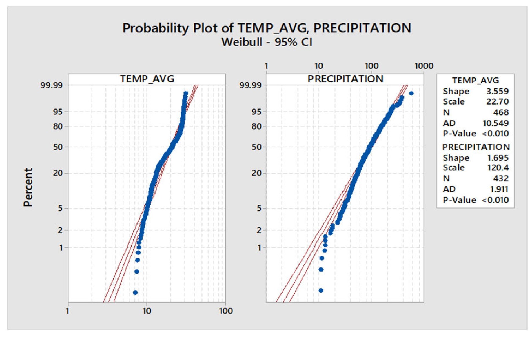
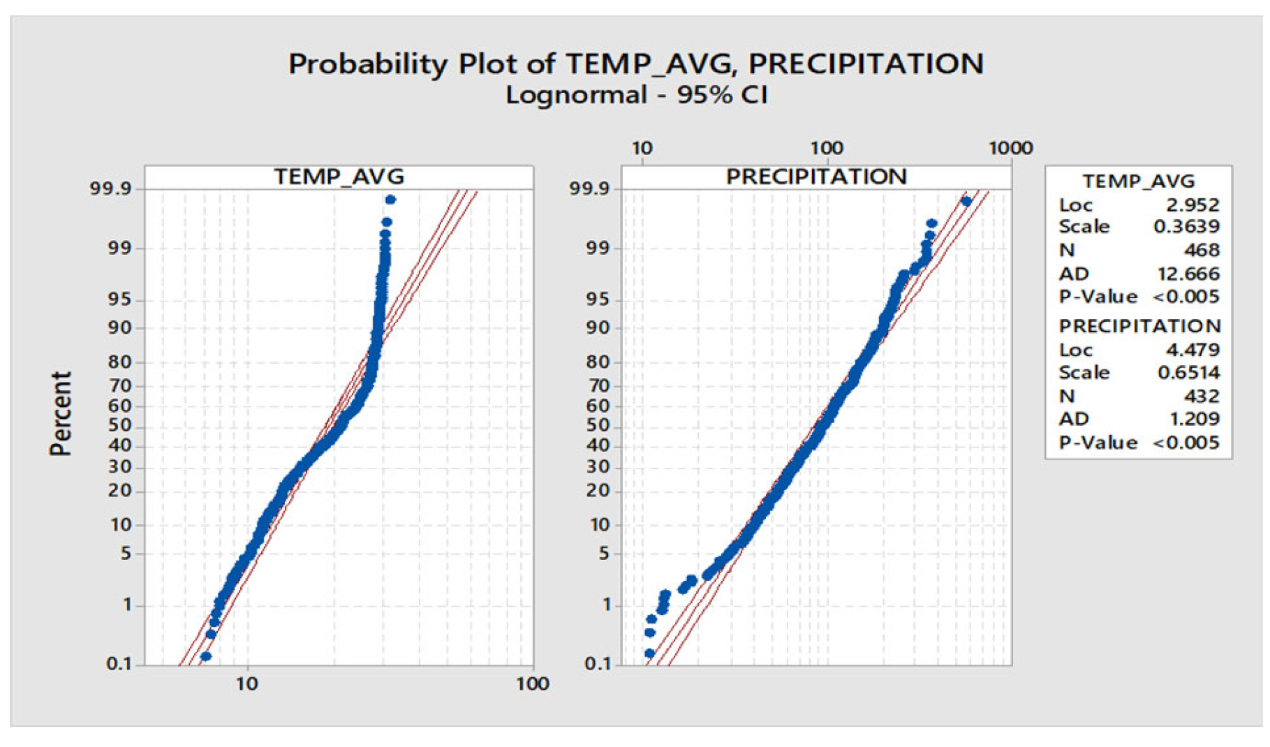
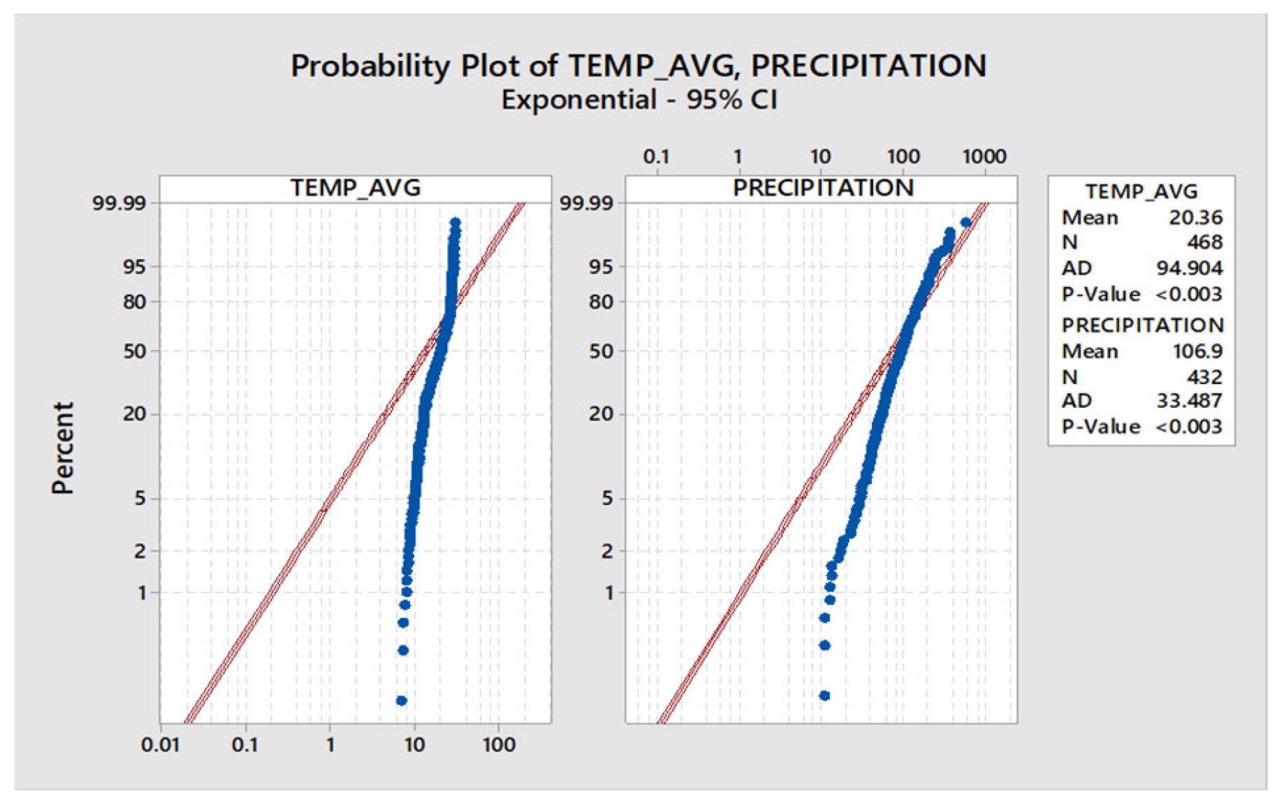
As the data set is huge, a statistical distribution study has been done. For this under 95% confidence interval, Normal distribution, Weibull distribution, Lognormal distribution and Exponential distribution has been tested for both temperature and precipitation data. In
Figure 1,
Figure 2,
Figure 3 and
Figure 4, it has been shown. Mainly, mean value, standard deviation, P value has been considered for the temperature and precipitation value. Among all four distribution we found that Weibull distribution has provided the best result according to the P value.
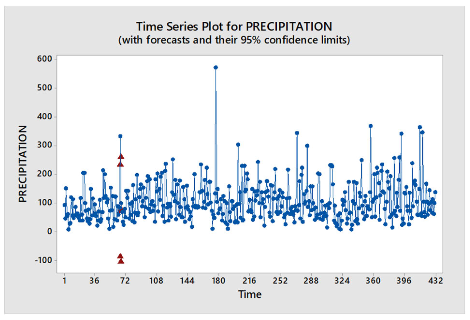
A time series plot has been done to observe precipitation pattern over time in
Figure 5.
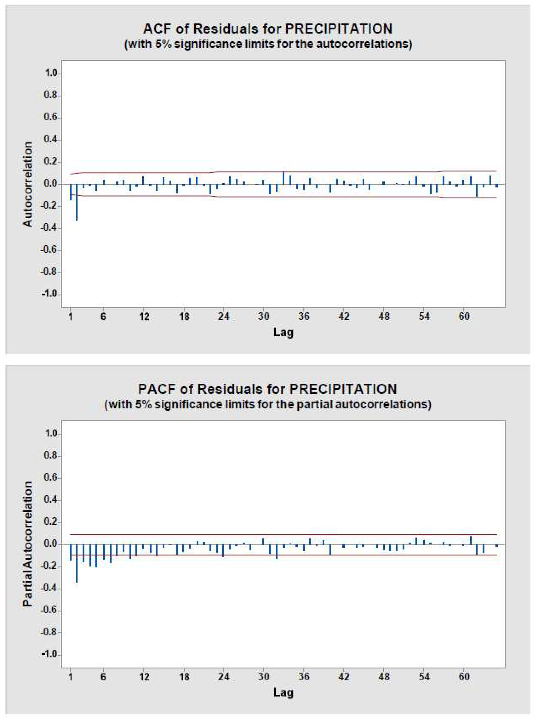
In
Figure 6, ACF (auto correction function) and PACF (partial auto correction function) residuals has been plotted for precipitation.
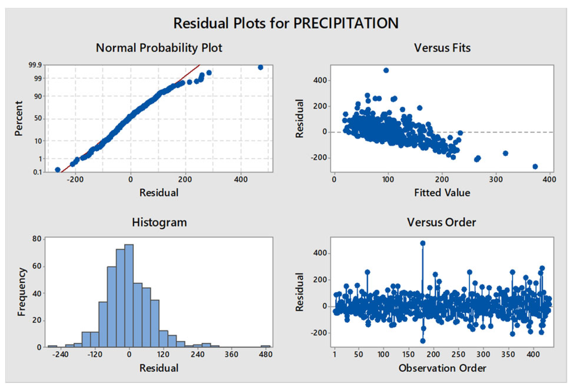
In
Figure 7: Residuals for precipitation has been shown where’re normal probability plot, residual vs fitted value, histogram and versus order have been shown for precipitation.
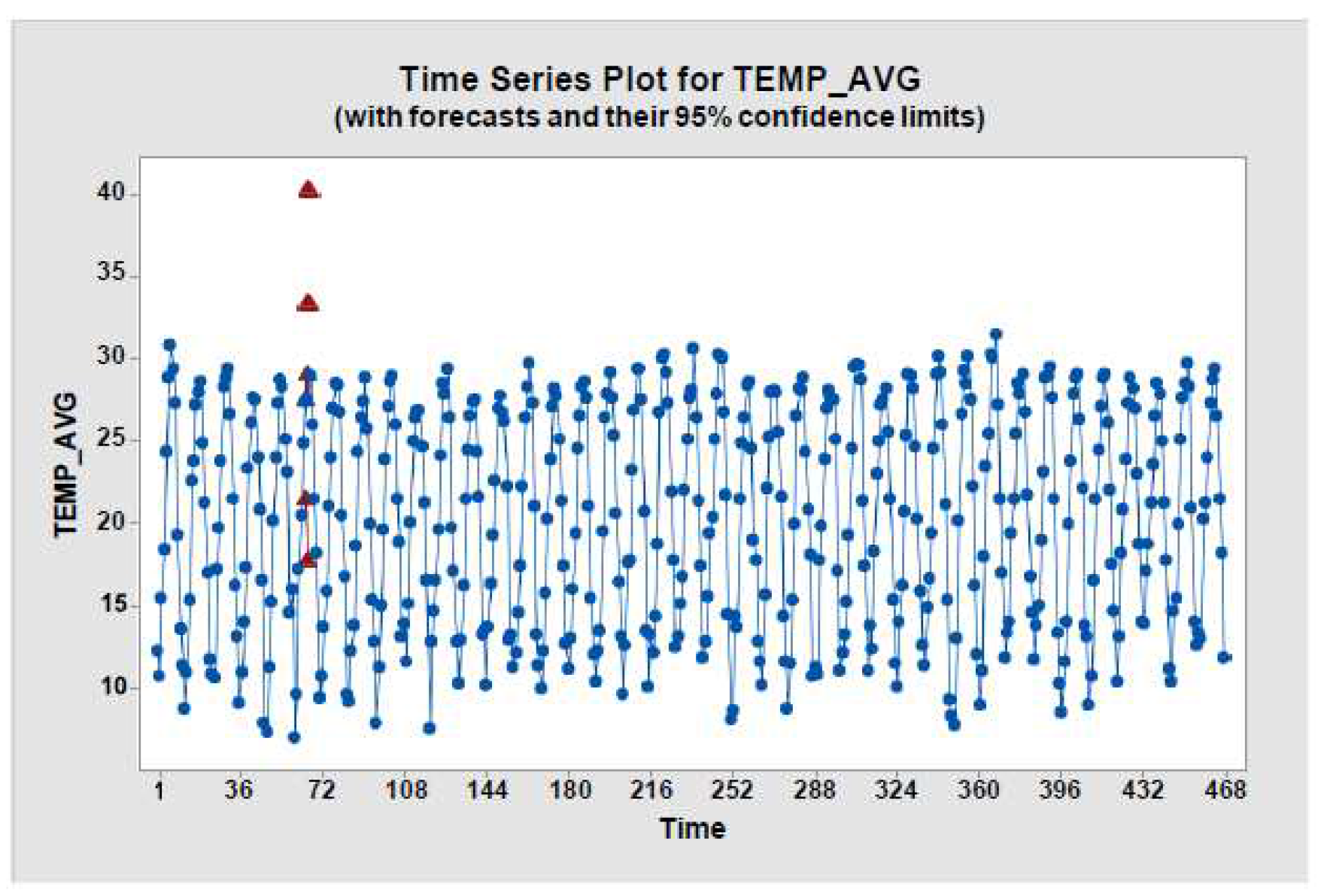
In
Figure 8, time series plot for average temperature has been plotted to get an idea of temperature change over a certain time period.
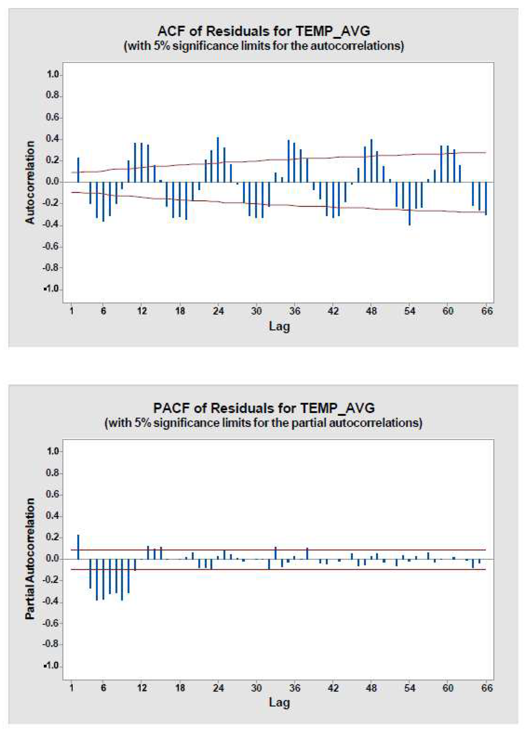
In
Figure 9: ACF and PACR of residuals has been plot for average temperature.
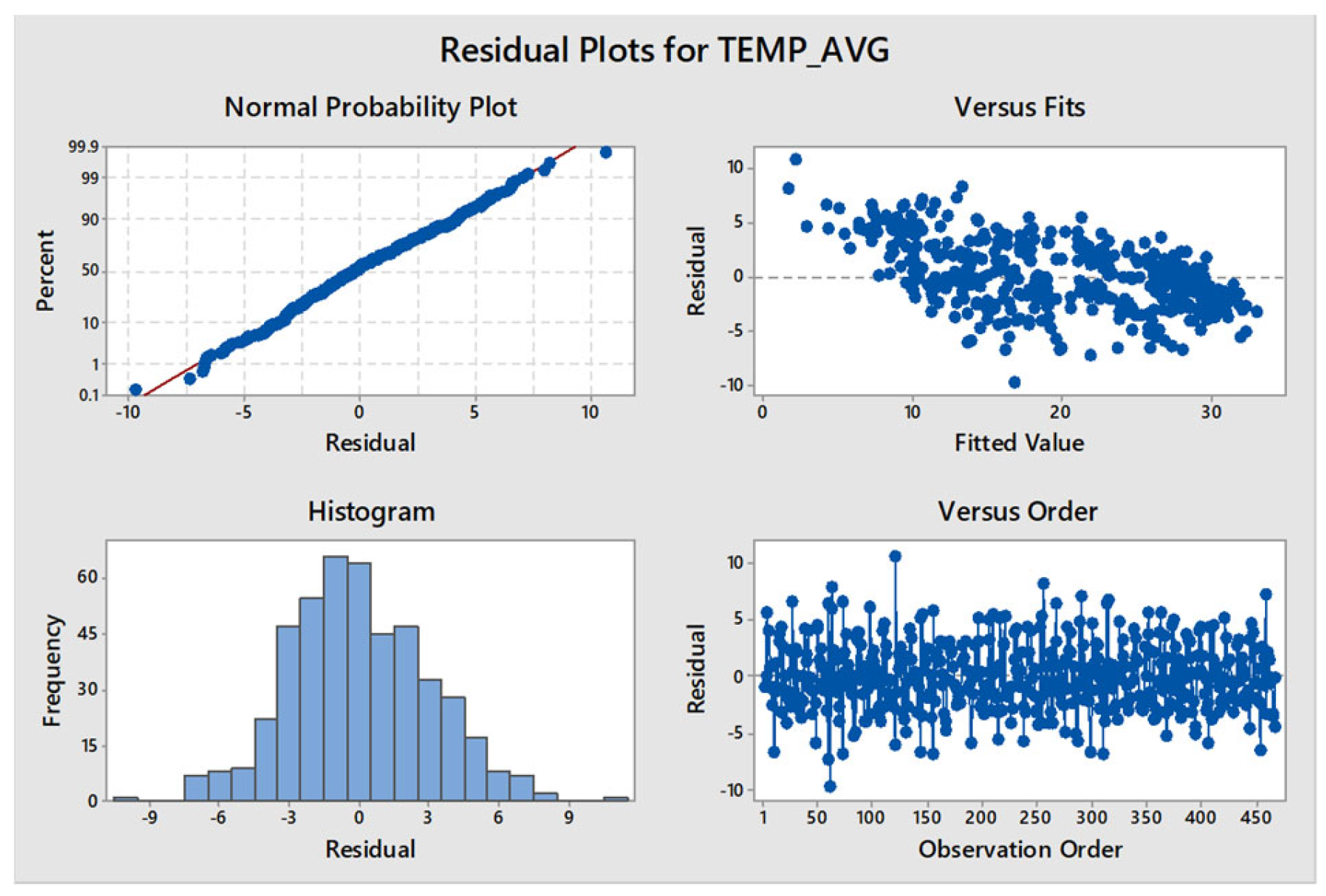
In
Figure 10: residual plots have been generated for average temperature where percent vs residual plot, versus fits, versus order and histogram have been plot.
Iteration SSE Parameters
| 0 5948.33 |
0.100 |
0.089 |
| 1 5088.33 |
0.250 |
0.063 |
| 2 4527.71 |
0.400 |
0.036 |
| 3 4266.46 |
0.550 |
0.009 |
| 4 4245.69 |
0.603 |
-0.007 |
| 5 4245.63 |
0.606 |
-0.010 |
| 6 4245.63 |
0.606 |
-0.010 |
| 7 4245.63 |
0.606 |
-0.010 |
Relative change in each estimate less than 0.0010 Final Estimates of Parameters
Type Coef SE Coef T P AR 1 0.6058 0.0371 16.34 0.000
Constant -0.0104 0.1398 -0.07 0.941
Differencing: 1 regular difference
Number of observations: Original series 468, after differencing 467 Residuals: SS = 4245.13 (backforecasts excluded)
MS = 9.13 DF = 465
Modified Box-Pierce (Ljung-Box) Chi-Square statistic Lag 12 24 36 48
Chi-Square 370.0 788.8 1201.9 1609.0
DF 10 22 34 46
Forecasts from period 65
95% Limits
Period Forecast Lower Upper Actual 66 27.3945 21.4712 33.3178 27.3000
67 28.9558 17.7507 40.1609 27.4000
5. Result from ARIMA model for Precipitation
Iteration SSE Parameters
| 0 5948.33 |
0.100 |
0.089 |
| 1 5088.33 |
0.250 |
0.063 |
| 2 4527.71 |
0.400 |
0.036 |
| 3 4266.46 |
0.550 |
0.009 |
| 4 4245.69 |
0.603 |
-0.007 |
| 5 4245.63 |
0.606 |
-0.010 |
| 6 4245.63 |
0.606 |
-0.010 |
| 7 4245.63 |
0.606 |
-0.010 |
Relative change in each estimate less than 0.0010 Final Estimates of Parameters
Type Coef SE Coef T P AR 1 0.6058 0.0371 16.34 0.000
Constant -0.0104 0.1398 -0.07 0.941
Differencing: 1 regular difference
Number of observations: Original series 468, after differencing 467 Residuals: SS = 4245.13 (backforecasts excluded)
MS = 9.13 DF = 465
Modified Box-Pierce (Ljung-Box) Chi-Square statistic Lag 12 24 36 48
Chi-Square 370.0 788.8 1201.9 1609.0
DF 10 22 34 46
Forecasts from period 468
95% Limits
Period Forecast Lower Upper Actual 469 75.386 64.048 87.821 76.310
470 80.542 70.953 96.037 77.500
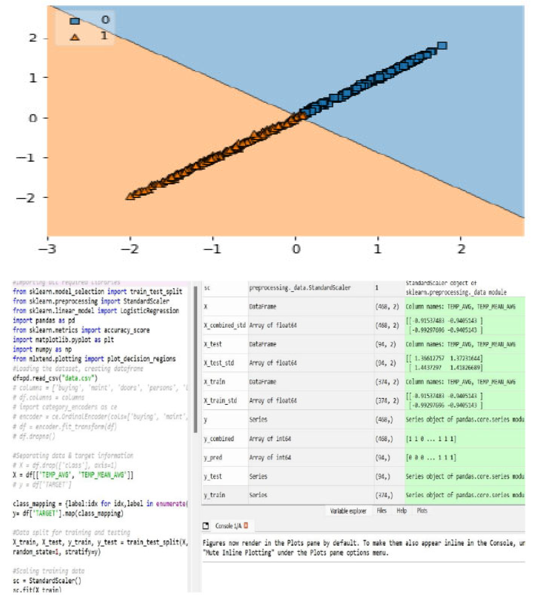
A logistic regression model has been generated. Among 468 data set, 374 data have been used to train the model and 94 set of data was used to test the model. The test value chart has been shown in
Figure 11.
6. Conclusion
From ARIMA model, 2 periods of data (per period 12 months) both for temperature and precipitation has been generated. After analyzing this data, from our developed Logistic Regression Model, it has found that both will have a negative effect on pavement performance. From the training, it has found that the regression model gives an idea if a value of temperature and precipitation has been given to the model. Since the model has been developed over a small scale of data, the output result accuracy will not be the desired one.
Recommendation from this study:
In the prediction model, there is substantial variation in terms of the magnitude.
No specific pavement damage has been mentioned
Only Yes or No condition is not enough for the data projection.
A clear matrix should be generated with pavement distress which will give us a high accuracy projection.
Long series of data set is recommended to train the mathematical model to get a better projection
References
- M. Rummukainen, “Changes in climate and weather extremes in the 21st century,” Wiley Interdisciplinary Reviews: Climate Change, vol. 3, no. 2, pp. 115–129, 2012.
- P. V. Hung and N. T. Thanh, “Asphalt Pavement Performance in Extreme Weather Events in Tropical Country,” International Journal of Engineering and Technical Research, vol. 8, no. 05, pp. 76–82, 2019.
- A. Dawson, “Anticipating and responding to pavement performance as climate changes,” in Climate change, energy, sustainability and pavements, Springer, 2014, pp. 127–157.
- F. De Longueville, Y.-C. Hountondji, I. Kindo, F. Gemenne, and P. Ozer, “Long-term analysis of rainfall and temperature data in Burkina Faso (1950–2013),” International Journal of Climatology, vol. 36, no. 13, pp. 4393–4405, 2016.
- J. C. Petersen, “Chemical composition of asphalt as related to asphalt durability,” in Developments in petroleum science, vol. 40, Elsevier, 2000, pp. 363–399.
- S.-S. Kim, S. Sargand, and A. Wargo, “A simple test procedure for evaluating low temperature crack resistance of asphalt concrete.,” Ohio Research Institute for Transportation and the Environment, 2009.
- Gadalla, “The Effects of Extreme Weather Events on Flexible Pavement,” 2020.
- Pagotto, M. Legret, and P. Le Cloirec, “Comparison of the hydraulic behaviour and the quality of highway runoff water according to the type of pavement,” Water Research, vol. 34, no. 18, pp. 4446–4454, 2000.
- E. A. E.-M. Behiry, “Laboratory evaluation of resistance to moisture damage in asphalt mixtures,” Ain Shams Engineering Journal, vol. 4, no. 3, pp. 351–363, 2013.
- X. Luo, F. Wang, H. Gong, J. Tao, X. Qiu, and N. Wang, “Effectiveness Evaluation of Preventive Maintenance Treatments on Asphalt Pavement Performance Using LTPP Data,” International Journal of Pavement Research and Technology, pp. 1–16, 2021.
|
Disclaimer/Publisher’s Note: The statements, opinions and data contained in all publications are solely those of the individual author(s) and contributor(s) and not of MDPI and/or the editor(s). MDPI and/or the editor(s) disclaim responsibility for any injury to people or property resulting from any ideas, methods, instructions or products referred to in the content. |
© 2024 by the authors. Licensee MDPI, Basel, Switzerland. This article is an open access article distributed under the terms and conditions of the Creative Commons Attribution (CC BY) license (http://creativecommons.org/licenses/by/4.0/).

