1. Introduction
Interval type-3 (IT3) fuzzy logic systems (FLS) represent a very handy technology according to the state-of the-art literature [
1,
2,
3,
4], [
5,
6,
7,
8,
9,
10,
11,
12,
13,
14,
15,
16,
17,
18,
19,
20,
21,
22,
23,
24,
25,
26,
27,
28,
29,
30,
31,
32,
33,
34,
35,
36,
37,
38,
39,
40]. Nowadays, the implementation of IT3 FLS in real life problems is a blank field given the complications presented in this model that is analogous to the general type-2 (GT2) FLS based on the definition in [
32]:
Definition 1. “The type-3 FLS, is the generalization of the type-2 FLS that has more capacity to cope with uncertainties. In T3-FLSs, the secondary membership function (MF) is also a type-2 MF. Then the upper and lower bounds of memberships are not constant in contrast to the type-2 MFs. These features cause more levels of uncertainties and can be handled by type-3 MFs. [32, p. 154]”
According to the previous definition and the analogy between the GT2 and IT3 systems, both adhere to the mathematical and methodological principles and to the challenges, difficulties, strengths, and weaknesses that authors defined as complications to face this class of systems [
5]. A comprehensive list of challenges to be faced is presented in [
41] and are shown in
Table 1.
A brief survey of the state-of-the-art literature shows that the found applications are only from the theoretical point of view of singleton (IT3 SFLS) [
3,
6,
7,
8,
9,
10,
11,
12,
13,
14,
15,
16,
17,
18,
19,
20,
21,
22,
23,
24,
25,
26,
27,
28,
29,
31,
32,
33,
34,
35,
36,
37,
38,
39,
40] and of type-1 non-singleton (IT3 NSFLS-1) FLS [5, 28 and 29]. This technology presents some challenges and complications in the design and implementation processes. i.e., in [
28] the development of a new flowmeter fault detection approach based on optimized non-singleton type-3 (NT3) FLS with type-1 non-singleton inputs is presented. The introduced method is implemented on an experimental gas industry plant. The system is modeled as NT3 FLS system, and the faults are detected by the comparison of measured and estimated signals. According to the authors, the level of non-singleton fuzzification and membership parameters are tuned by a maximum correntropy (MC) unscented Kalman filter (KF), and the rule parameters are learned by correntropy KF (CKF) with fuzzy kernel size.
In contrast to the recent developments on automata’s, drones, automated remote vehicles (ARV’s) among others, require adaptation, learning, tuning to get the necessary knowledge for adaptation to the changing environments, the applications of IT3 are limited and their analogy with GT2 systems exists as it is documented in [
5], e.g., the GT2 NSFLS-1 is used as a controller for control and balance a two-wheel mobile robot [
54]. The GT2 NSFLS-1 model is used in a proportional, integral, and derivative (PID) controller to get effectiveness and robustness in a plan controller affected by external disturbances [
55].
The GT2 NSFLS-1 model is used to manage efficient and energy conserving permanent magnetic drive [
56]. In [
57] the GT2 NSFLS-1 is proposed to test and to provide a theoretical framework using the enhanced Karnik-Mendel Algorithm and the Nie-Tan algorithm to see their accuracy. In [
58] it is presented an adaptive GT2 non-singleton fuzzy neural network control for motion balance adjusting of a power-line inspection robot. In [
59] are presented GT2 NSFLS-1 classifiers for medical diagnosis. A medical application to regulate glucose levels is proposed in [
60]. In [
61] it is presented a model to synchronize chaotic systems affected by external disturbances.
The difficulties presented in
Table 1 happen in the GT2 and IT3 singleton fuzzy systems in both, Mandami and Takagi-Sugeno-Kang (TSK) models, and it is remarkable that happens in the singleton form that is the simplest or primitive form of fuzzy systems, in [
41,
42,
43,
44,
45,
47,
48,
49,
50,
51,
60,
61,
62,
63,
64,
65,
66,
67,
68,
69,
70,
71,
72,
73,
74,
75,
76,
77,
78,
79,
80,
81,
82,
83,
84,
85,
86,
87,
88,
89,
90] for GT2 FLS and [
91,
92,
93,
94,
95,
96,
97,
98,
99,
100,
101,
102,
103,
104,
105,
106,
107,
108,
109,
110,
111,
112,
113,
114,
115,
116,
117] IT3 FLS. In contrast for the case of the IT3 type-1 non-singleton systems there are only a limited number of applications [19, 20, 29 and 40] and for IT3 type-2 non-singleton there is only one, [
5]. In
the state-of-the-art modern literature, the reference to IT3 NSFLS-1 and to IT3 NSFLS-2 is practically inexistent but in contrast the synonym (generalized type-2 non-singleton) used for this technology of knowledge acquisition for tuning, adaptation, updating, learning, or training shows that from 2021 until now there are 44 papers that include proposals with type-3 fuzzy logic systems. There are 39 publications named as “shadowed type-2” fuzzy systems. Using the “knowledge acquisition” there are 10 papers with learning, 8 papers with tuning, 11 papers for adaptation and only four papers for updating, as shown on Table 2. Table 3 shows the literature on IT3 FLS in their singleton and non-singleton versions with 52 papers of type-3 fuzzy logic systems. For knowledge acquisition there are 4 papers with hybrid learning, 38 papers with learning, and 33 papers with tuning, 30 papers for adaptation and only 5 papers for updating, one or more of these terms are mentioned in the same paper.
The few applications found in the state-of-the-art literature, the difficulties in optimizing the models, the fact of multiple calculation to obtain several numbers of planes as mentioned in [
83] and the requirement of iterative methods to train the model have led researchers to use different models which stand out principally in GT2 SFLS systems for acquiring knowledge, learning, and tuning in their different definitions.
To the best of the authors' knowledge, studies of GT2 NSFLS-1 and IT3 NSFLS-1 that use the OLS-BP hybrid learning mechanism as a training method have not been found in the state-of-the-art literature. However, there are publications presented elsewhere referring to the IT2 Mamdani FLS [
118,
119,
120,
121], and to the IT2 TSK FLS [
122,
123] using the proposed hybrid OLS-BP mechanism.
As mentioned earlier, the intention of this article is to present and discuss the proposed OLS-BP hybrid learning algorithm for antecedent and consequent parameter tuning of the novel Enhanced Wagner-Hagras (EWH) IT3 NSFLS-1 system and demonstrate its implementation in a real industrial hot strip mill (HSM) application. To enable direct comparison of the performance and functionality of the proposed hybrid mechanism, the same input-output data set is used as in [
118,
119,
120,
121,
122,
123] and it has been experimentally examined under the same conditions as in previous work.
The main contributions of this proposal are:
1. The detailed mathematical formulation of the hybrid OLS-BP training method using a) the partial derivatives with respect to a performance criterion to tune each parameter for only the antecedent section of the level- and b) the orthogonal transformations of rotation or OLS method to tune only the consequent parameters of the level- of the proposed enhanced WH system. This system is named as hybrid enhanced EWH IT3 NSFLS-1 (OLS-BP) fuzzy system.
2. A more precise and economical method to estimate the final value using the simply average of the outputs of the EWH IT3 NSFLS-1 (OLS-BP) fuzzy system, which includes the horizontal level- or IT2 FLS output, , calculated as , instead of the classic WH method using the weighted average: .
3. The use of the alternative method to construct the EWH IT3 NSFLS-1 system with dynamical structure, where each of its
horizontal levels-
has its own base of
rules. The output
of each level-
is calculated using the antecedent’s firing interval
and the consequent’s centroid
of each
th rule. According to the WH method for the construction of the EWH IT3 NSFLS-1 system, [
5], each output
of each level-
is calculated using the estimation of the
-cuts at level-
. The present proposal does not estimate each
-cut of each input
at each level-
, that is the
interval values, in order to calculate the firing interval values
of this level-
. This proposal estimates both, the antecedent firing levels
and the consequent centroids
using a Gaussian models as a secondary membership functions.
4. To the best knowledge of the authors, this is the first time that the hybrid EWH IT3 NSFLS-1 (OLS-BP) fuzzy system is applied to predict the transfer bar surface temperature at the entry zone of the finishing scale breaker of a HSM.
This work is organized as follows. In
Section 2 the foundations of the proposed EWH IT3 FLS systems, the BP, and the OLS training methods are exposed to let the reader contextualize the proposal also presented in this section.
Section 3 presents the application and validation of the performance of the proposed methodology applied to the temperature prediction of the transfer table of the host strip mill facility.
Section 4 presents the results analysis obtained in the application. Finally, Section 5 provides the conclusions.
3. Results and Discussion
3.1. The Problem: Industrial Process Description
The HSM process presents many complexities and uncertainties involved in rolling operations.
Figure 10 shows the HSM sub-processes: The reheat furnace, the roughing mill (RM), the transfer tables, the scale breaker (SB), the finishing mill (FM), the round out tables, and the coiler (CLR).
The most critical subprocess is the FM. There are several mathematical model-based systems for setting up the FM, which calculate the working references required to obtain the target strip gauge, target strip width and target strip temperature at the exit zone of the FM. The math model takes as inputs the FM target strip gage, the target strip width, the target strip temperature, the slab steel grade, the hardness ratio from slab chemistry, the FM load distribution, the FM gauge offset, the FM temperature offset, the FM roll diameters, the FM load distribution, the input transfer bar gauge, the input transfer bar width, and the most critical variable, the input transfer bar temperature.
The math model requires knowing accurately what the input transfer bar temperature is at the entry zone of the FM. A minimum entry temperature error will propagate through the entire FM and produce a coil out of the required quality. For the estimation of this FM entry temperature, the math models require knowledge of the transfer bar surface temperature, which is measured by a pyrometer located at the RM exit side, and knowledge of the time taken to translate the transfer bar from the RM exit zone to the FM SB entry zone.
These pyrometer's measurements are affected by the noise produced by the surface scale growth, environment water steam, the pyrometer’s location, calibration, resolution, repeatability, and by the recalescence phenomenon occurring at the RM exit in the body of the transfer bar [
126]. The time required by the transfer bar to move its head end from the RM exit to the FM entry zones, is estimated by the math model. This time estimation is affected by the free air radiation phenomenon occurring during the transfer bar translation and by the inherent uncertainty of the kinematic and dynamic modeling.
The math model parameters are adjusted using both the uncertain surface temperature measured by pyrometers located at the FM entry zone, and the uncertain surface temperature at the FM entry zone estimated by the model. The proposal estimates the input transfer bar temperature at the entry zone of the FM and was off-line tested using real data from an industrial HSM facility located in Monterrey, México, which is currently using a certain type of fuzzy system for this estimation.
3.2. Simulation
This section presents the experimental testing of the proposal, the prediction of the transfer bar surface temperature.
3.2.1. Input-output Data Pairs
From an industrial HSM process, one hundred and seventy-five noisy input-output data pairs of three different types of coils,
Table 7, were obtained and used as offline training data,
. The inputs were
, the transfer bar surface temperature measured by the pyrometer is located at the RM exit zone, and
, the real time to move the transfer bar end from the RM exit zone to the SB entry zone. The output
y was the transfer bar surface temperature measured by the pyrometers located at the SB entry zone and used to calculate the temperature prediction error.
3.2.2. Antecedent Membership Functions
The primary membership functions for each antecedent of the base IT2
NSFLS-2 system were Gaussian functions with uncertain means
,
, and with the standard deviation
, as shown in
Table 8 and
Table 9. An array of two inputs, with five MF each, produces
rules.
3.2.3. Fuzzy Rule Base
The EWH IT3 NSFLS-1 fuzzy rule base consists of a set of IF-THEN rules that represent the model of the complete system. The IT2
NSFLS-1, that is the base of the 3D construction of the proposed fuzzy system, has two inputs
and
and one output
. The rule base has
rules of the type shown in
Table 10.
3.3. Results and Discusion
Three different sets of data for three different coil types were taken from a real mill. Each of these data sets was split into two sets: One for the initial adjustment and tuning process, and the other for the setup validation process. Eighty-three of type A, sixty-five of type B and twenty-seven of type C input-output data pairs were used for the initial offline training process, and seven input-output data pairs were used for testing. The production gage and width coil targets of the training data with the steel grade are shown in
Table 7. A Dell PC i7, 16 GB RAM memory and 2.8 GHz using Win 11 OS was used to execute the fuzzy systems programed in MS VS 2022 C++ language.
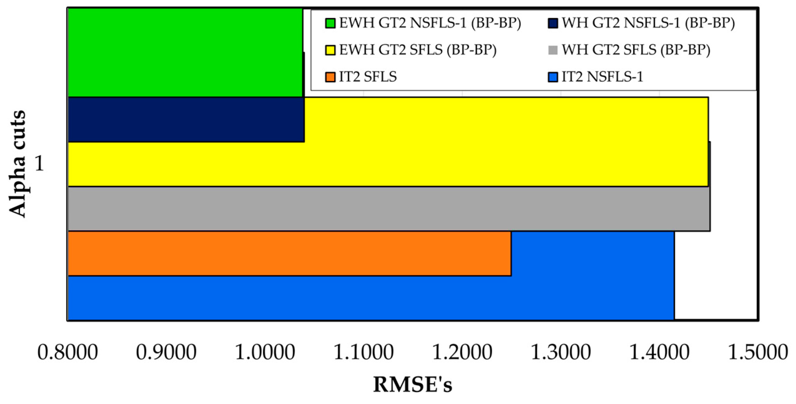
Seven input-output data pairs were used to test the offline SB entry temperature estimation. The Root Mean Square Error (RMSE) for the prediction obtained with GT2 models trained with the BP-BP algorithm and IT2 systems used as benchmark models and the proposed EWH algorithm with BP-BP using only one
-cuts are shown in
Table 11 and
Figure 11. The EWH algorithm shows an enhancement of 0.2 % versus the classic WH model using BP-BP learning model for the GT2 SFLS systems. On other hand, the WH algorithm using IT3 SFLS models show an enhancement of 0.36% for classic WH singleton and 0.41% the EWH proposed algorithm in singleton compared with the IT2 singleton model as shown in
Table 12 and
Figure 12.
For non-singleton cases, both models, WH and EWH, present the same prediction in the case of the GT2 models. In contrast the IT3 models show a bigger enhancement versus the IT2 NSFLS-1 models. In the first case the WH IT3 NSFLS-1 (BP-BP) show an enhancement of 22.5 % for the WH algorithm and 30.2% for the EWH proposed algorithm as shown in
Table 12 and
Figure 12.
The RMSE prediction of the GT2 and the proposed EWH algorithm using different levels-
as shown in
Table 13 and
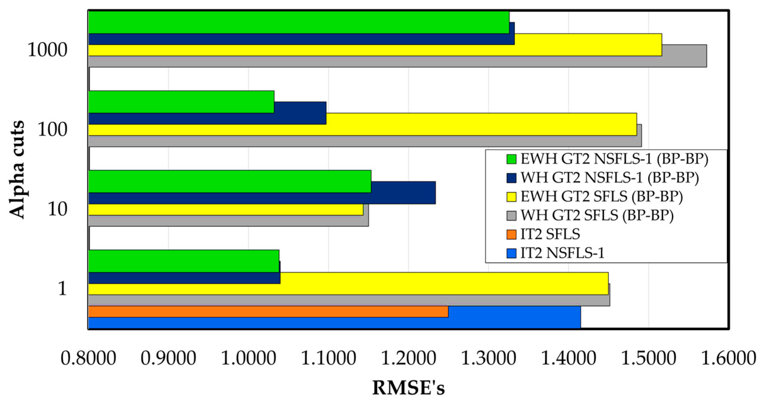
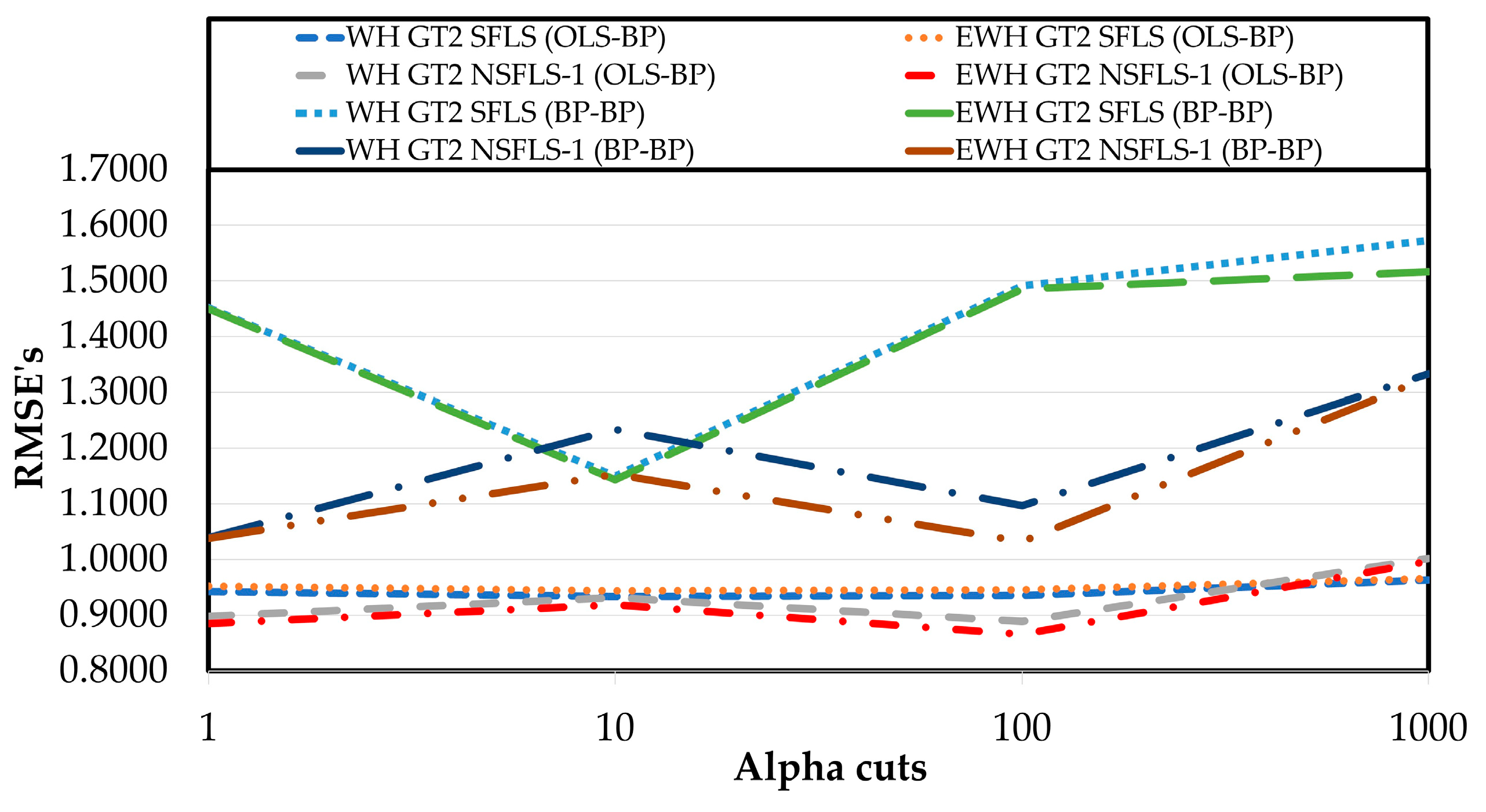
Figure 13, show that the GT2 SFLS-1 (BP-BP) with the proposed model (EWH) outperforms the WH GT2 SFLS with only 10
-cuts in an order of 19.1% for WH GT2 singleton with BP-BP learning algorithm and 19.5% for the IT3 with the EWH algorithm with BP-BP learning as is shown in
Table 14. On other hand, with the non-singleton models the enhancement is 2.3% for the WH algorithm and 17% for the EWH algorithm for both with BP-BP learning. The best results are obtained with 100
-cuts with an enhancement of 12.3% for the WH algorithm and 17.5% for the EWH algorithm, both with BP-BP learning as shown in
Table 13 and
Figure 13.
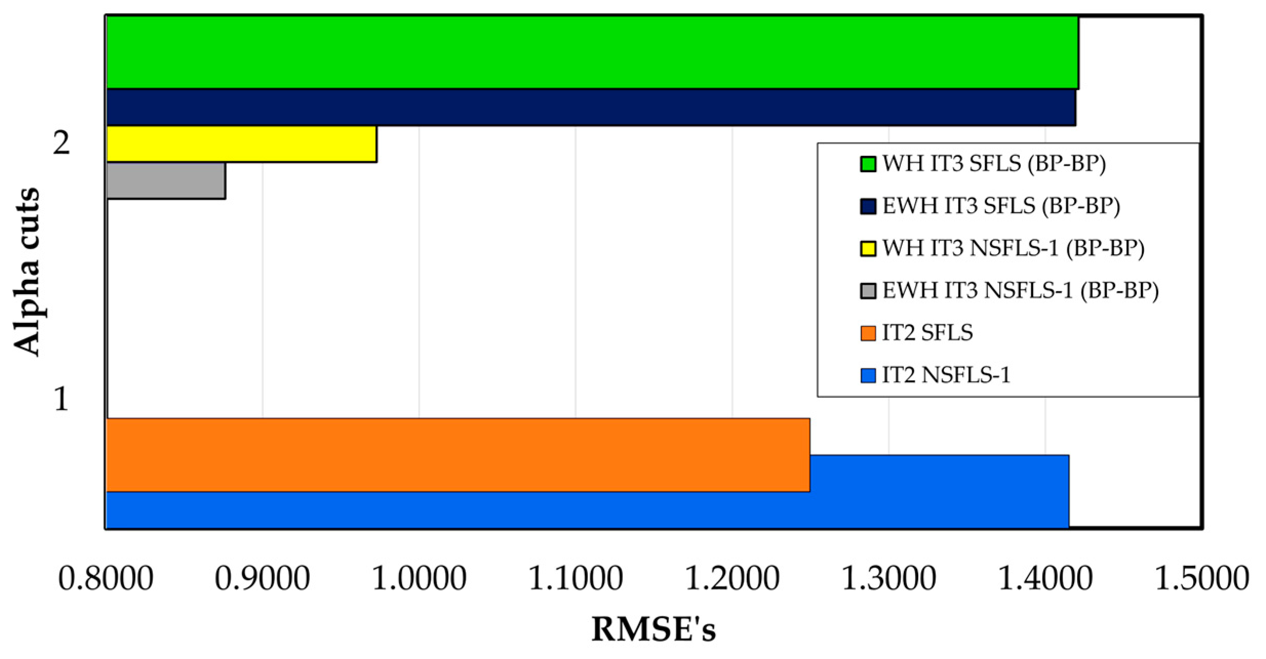
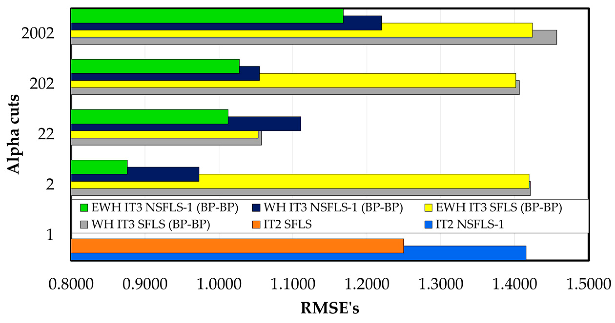
In contrast when the IT3 fuzzy systems are used the results show a reduction in the error rates in every number of
αk-cuts tested. E.g., with 202
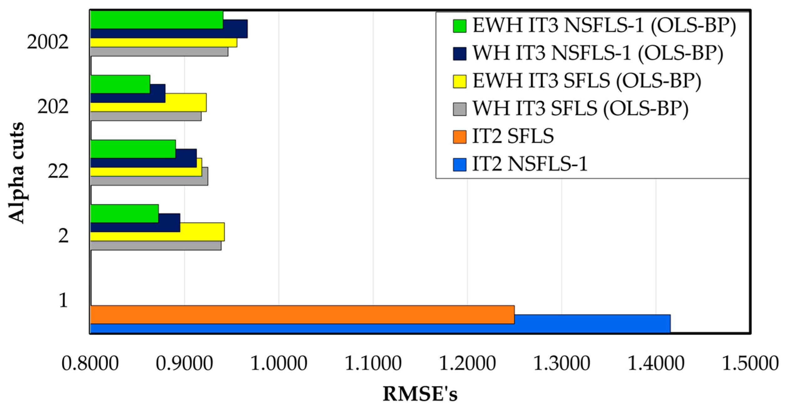
αk-cuts the enhancement versus the IT2 SFLS using the WH learning is in the order of 1.4%, and for the EWH IT3 NSFLS-1 (BP-BP) is in the order of 27.9% as it is shown in
Table 14 and
Figure 14.
Table 14.
Comparison between the benchmark models (IT2 SFLS and IT2 NSFLS-1) and IT3 models with BP-BP learning using the classic WH algorithm and the EWH algorithm with different number of -cuts.
Table 14.
Comparison between the benchmark models (IT2 SFLS and IT2 NSFLS-1) and IT3 models with BP-BP learning using the classic WH algorithm and the EWH algorithm with different number of -cuts.
|
-cuts |
1 |
2 |
22 |
202 |
2002 |
| IT2 SFLS |
1.4249 |
|
|
|
|
| IT2 NSFLS-1 |
1.2542 |
|
|
|
|
| WH IT3 SFLS (BP-BP) |
|
1.4212 |
1.0573 |
1.4063 |
1.4568 |
| EWH IT3 SFLS (BP-BP) |
|
1.4192 |
1.0528 |
1.4016 |
1.4239 |
| WH IT3 NSFLS-1 (BP-BP) |
|
0.9729 |
1.1107 |
1.0547 |
1.2197 |
| EWH IT3 NSFLS-1 (BP-BP) |
|
0.8761 |
1.0125 |
1.0275 |
1.168 |
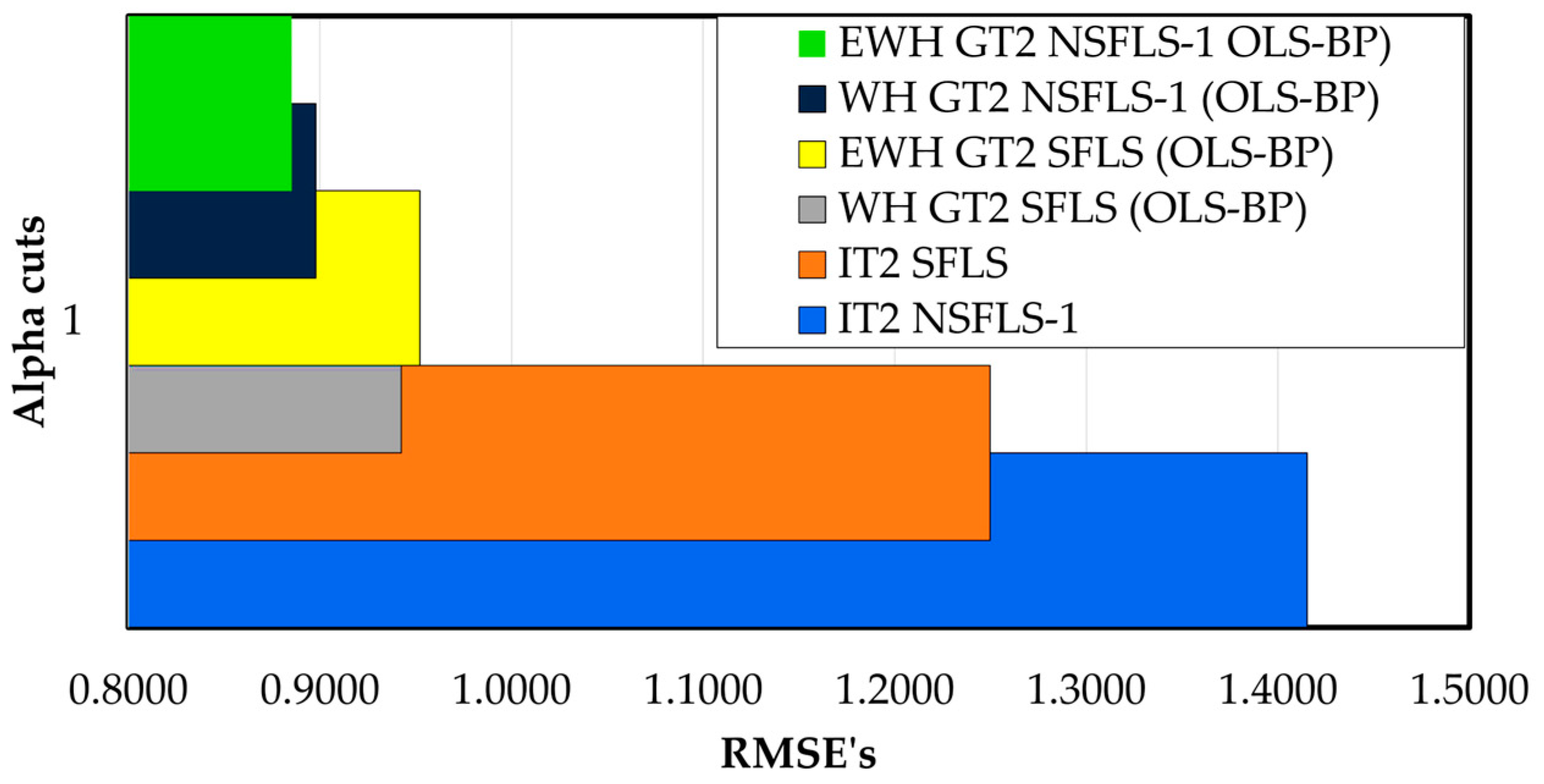
The values of the RMSE of the GT2 using the proposed hybrid learning (OLS-BP) with the WH and the proposed EWH are presented in Table 15 for only 1
αk-cut. Their results show an enhancement of 34.2 % comparing the IT2 SFLS with the WH GT2 SFLS using OLS-BP learning and shows an enhancement of 33.9 % when comparing the IT2 SFLS against EWH GT2 SFLS (OLS-BP) system (see
Table 15, and
Figure 15). The results show that the tested systems WH GT2 SFLS (OLSBP) and the EWH GT2 SLFS (OLS-BP) outperforms the IT2 SFLS with only 1
αk-cut. In a complementary form the WH GT2 NSFLS-1 (OLS-BP) presents an enhancement of 28.7% for the WH GT2 NSFLS-1 (OLS-BP) learning and 30.5% for the EWH GT2 NSFLS-1 (OLS-BP) system.
On other hand, the RMSE for the prediction using both the WH and the EWH IT3 models with the OLS-BP learning algorithms, shows that the error rates are reduced significantly to 34.2% for the WH IT3 SFLS (OLS-BP), 33.9% for the EWH algorithm in the IT3 SFLS (OLS-BP) as shown in
Table 16 and
Figure 16. For the IT3 with only two
αk-cuts the IT3 NSFLS-1 model presents continuous enhancements when compared with IT2 and with GT2 systems. The WH IT3 NSFLS-1 (OLS-BP) system presents better performance with a reduction of 28.7% and 30.5% for the EWH IT3 NSFLS-1 (OLS-BP) model, as shown in
Table 16 and
Figure 16.
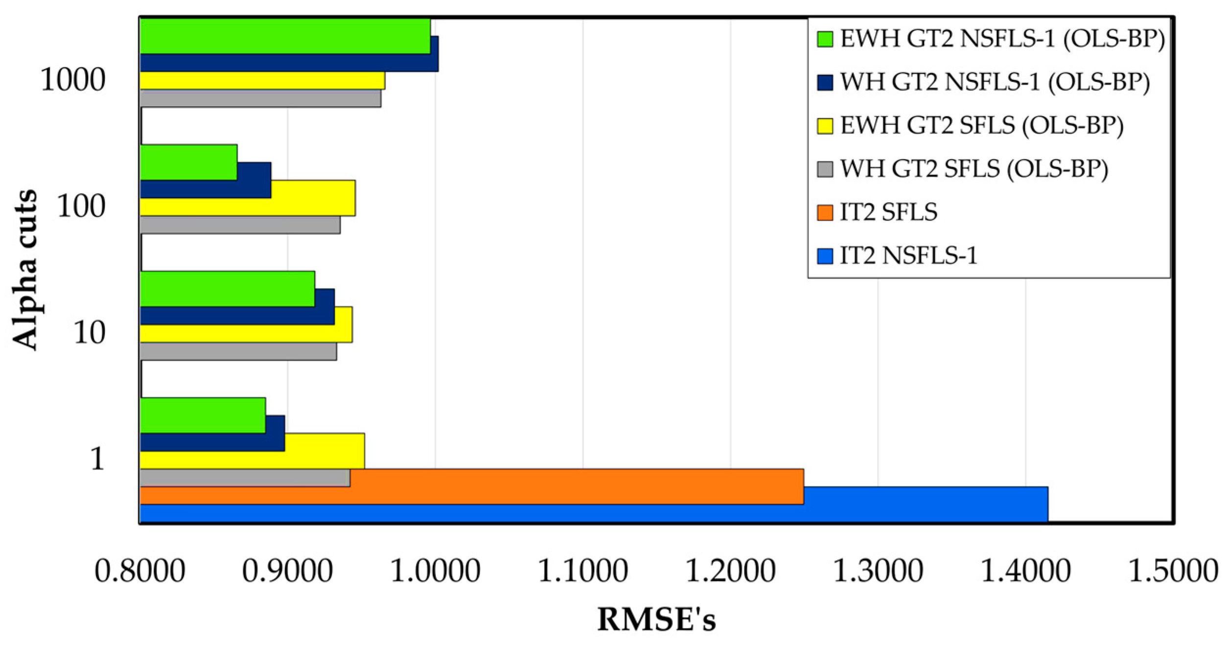
Table 17 shows the RMSE of the GT2 systems using the OLS-BP learning algorithm with different number of
αk-cuts. The results show a significant reduction versus the IT2 SFLS systems presenting a 34.2% in the comparison against WH GT2 SFLS (OLS-BP) learning and 33.9% against IT2 SFLS and for 33.2% for EWH GT2 SFLS (OLS-BP) system. In contrast, when comparing the non-singleton models it is obtained 38.5 % and 29.5 % for the WH GT2 NSFLS-1 (OLS-BP) and EWH GT2 NSFLS1 (OLS-BP), respectively. In a complementary form the WH GT2 NSFLS-1 (OLS-BP) presents an enhancement of 28.7% for the WH GT2 NSFLS-1 (OLS-BP) learning and 30.5% for the EWH GT2 NSFLS-1 (OLS-BP) system. Compared with the IT3 models, the RMSE showed a reduction on the error of prediction of 34.2% for WH IT3 SFLS (OLS-BP), 33.9% for EWH IT3 SLFS (OLS-BP) models. For non-singleton models a reduction of 38.7% for the IT3 NSFLS-1 (OLS-BP) and 30.15% against the IT2 NSFLS-1 were obtained, respectively.
Figure 17.
RMSE of prediction of GT2 systems with OLS-BP learning.
Figure 17.
RMSE of prediction of GT2 systems with OLS-BP learning.
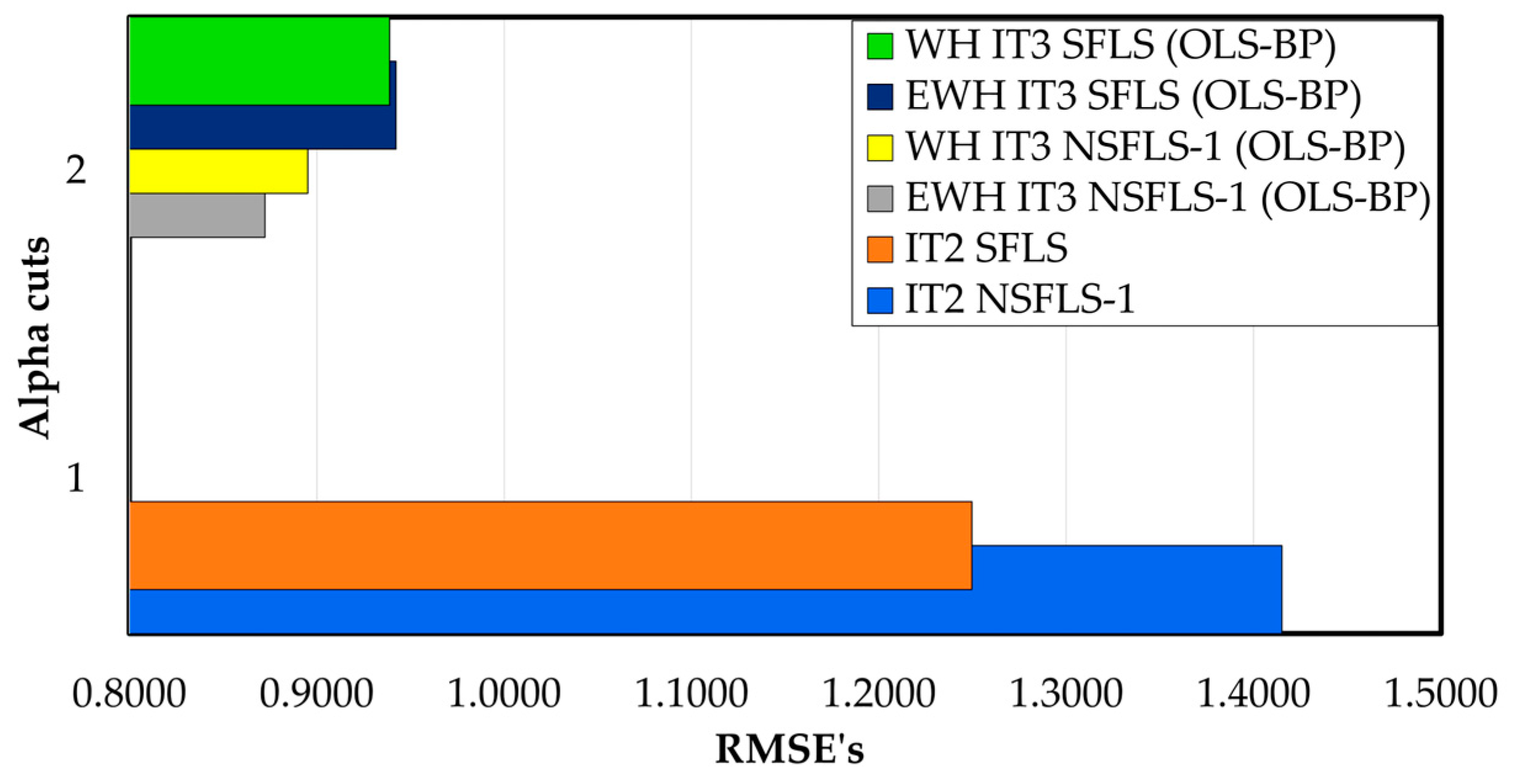
The values of RMSE prediction for the IT3 using the proposed learning OLS-BP with the WH algorithm and the proposed EWH algorithm are presented in
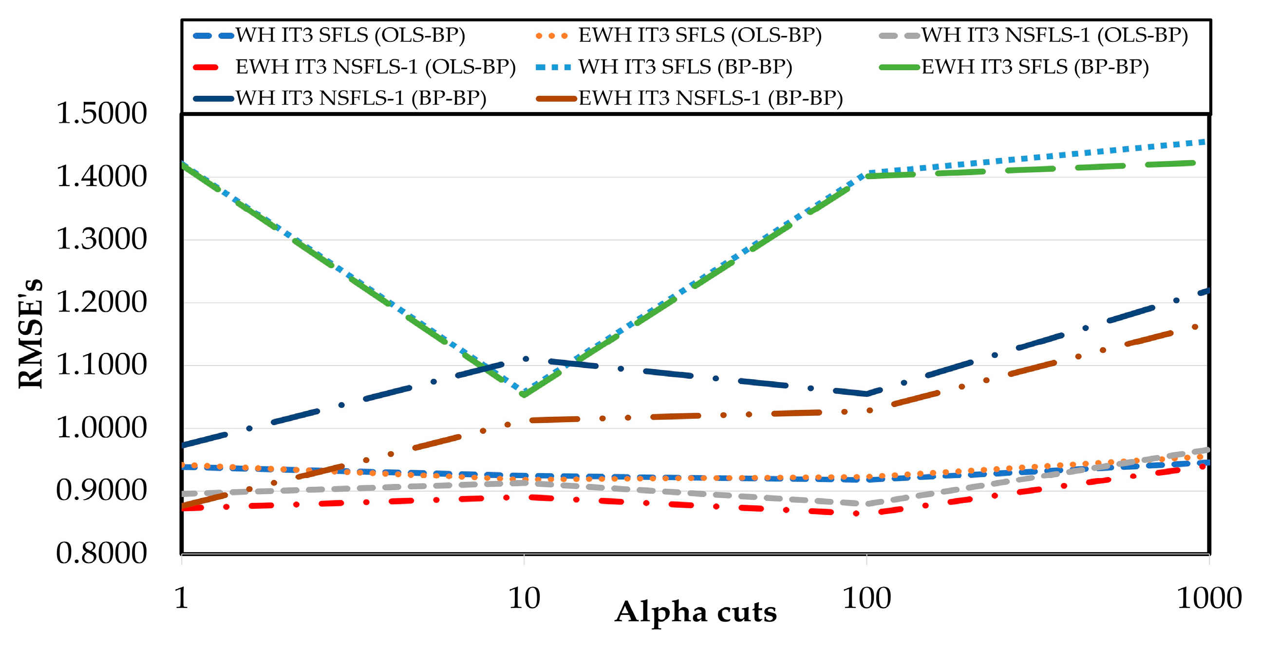
Table 18 using different quantities of
αk-cuts. The results show an enhancement of 34.2 % comparing the IT2 SFLS with the WH IT3 SFLS algorithm using OLS-BP learning. It also showed an enhancement of 33.9 % comparing the IT2 SFLS to the EWH IT3 SFLS (OLS-BP) system as shown in
Table 18 and
Figure 18, demonstrating that the tested systems WH IT3 SFLS (OLS-BP) and EWH IT3 SLFS (OLS-BP) outperforms the IT2 SFLS with only 2
αk-cuts.
For offline tuning, twenty training epochs were used with validated and bounded input-output data pairs, which guarantees the convergence of the proposed EWH IT3 NSFLS-1, as experimentally demonstrated in this research.
With the proposed OLS-BP hybrid training method, the IT3 NSFLS-1 was the one that presented the best performance. The results obtained by the GT2 systems are better than the IT2 models but, however, not better than the IT3 systems as shown in
Figure 19.
The results show that the best estimation is obtained by the proposed EWH IT3 NSFLS-1 (OLSBP) model using 202 levels-
α with a RMSE = 0.8634°C. The IT3 NSFLS-1 using any number of levels-
α presented the values of RMSE below to 1°C as shown in
Figure 20.
4. Conclusions
This work presents a novel hybrid learning method for parameter tuning of the novel EWH method for IT3 NSFLS-1 output estimation. The consequent parameters are tuned using the OLS training algorithm, while the antecedent parameters are tuned using the classic BP algorithm. The proposed EWH fuzzy systems use the average instead of the weighted average, to estimate the final output value of the fuzzy system, , where the contribution of the horizontal level- or IT2 FLS output, , improves the accuracy of this estimation. Each horizontal level- contributes 100% with its estimation of its output, .
The simulation results show that the proposed EWH IT3 NSFLS-1 (OLS-BP) hybrid algorithm produces better performance to generate better temperature estimation when compared with the BP-BP training. The better performance is obtained by the proposed EWH fuzzy systems when compared with the classic WH fuzzy systems. Also, the comparisons between several types of fuzzy systems showed that the IT3 NSFLS-1 are the best among the IT3 SFLS, GT2 NSFLS-1, GT2 SFLS, and the IT2 fuzzy systems.
For the future work, we plan to apply the hybrid algorithm and the EWH to the GT2 fuzzy systems and apply this system to FM exit gage, FM exit width, and FM exit temperature estimation of the head strip.
Author Contributions
For research articles with several authors, a short paragraph specifying their individual contributions must be provided. The following statements should be used “Conceptualization, Gerardo Mendez; Data curation, Gerardo Mendez, Ismael Lopez Juarez, Maria Alcorta Garcia and Pascual Montes Dorantes; Formal analysis, Gerardo Mendez, Ismael Lopez Juarez, Maria Alcorta Garcia, Dulce Martinez Peon and Pascual Montes Dorantes; Investigation, Gerardo Mendez, Maria Alcorta Garcia, Dulce Martinez Peon and Pascual Montes Dorantes; Methodology, Gerardo Mendez and Pascual Montes Dorantes; Project administration, Gerardo Mendez; Resources, Gerardo Mendez, Ismael Lopez Juarez, Maria Alcorta Garcia, Dulce Martinez Peon and Pascual Montes Dorantes; Software, Gerardo Mendez and Pascual Montes Dorantes; Validation, Gerardo Mendez, Ismael Lopez Juarez, Maria Alcorta Garcia, Dulce Martinez Peon and Pascual Montes Dorantes; Visualization, Gerardo Mendez, Ismael Lopez Juarez, Maria Alcorta Garcia, Dulce Martinez Peon and Pascual Montes Dorantes; Writing – original draft, Gerardo Mendez and Pascual Montes Dorantes; Writing – review & editing, Gerardo Mendez, Ismael Lopez Juarez, Maria Alcorta Garcia, Dulce Martinez Peon and Pascual Montes Dorantes. All authors have read and agreed to the published version of the manuscript.”.
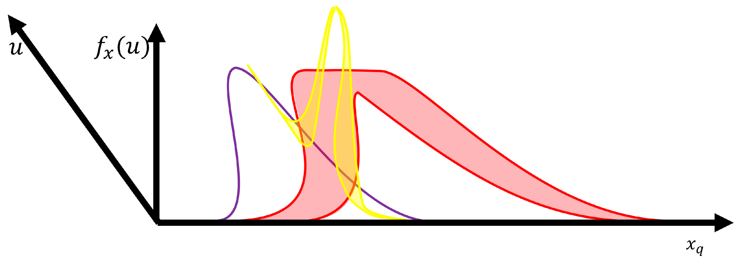
Figure 1.
Geometrical view of the GT2 NSFLS-1.
Figure 1.
Geometrical view of the GT2 NSFLS-1.
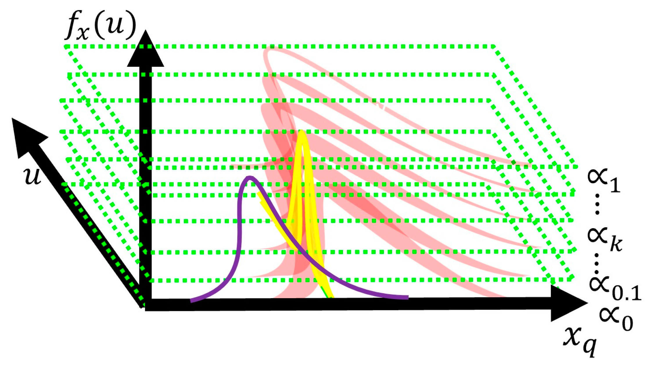
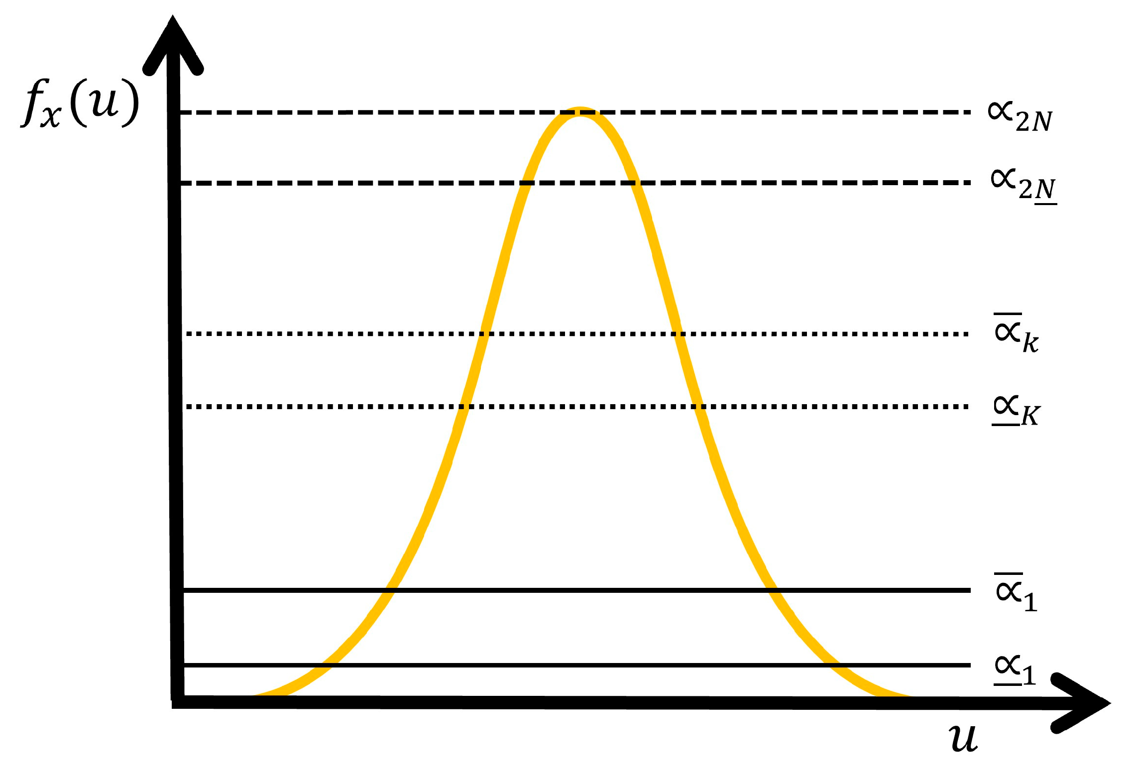
Figure 2.
Levels- and uncertain secondary values of the proposed EWH IT3 NSFLS-1 system.
Figure 2.
Levels- and uncertain secondary values of the proposed EWH IT3 NSFLS-1 system.
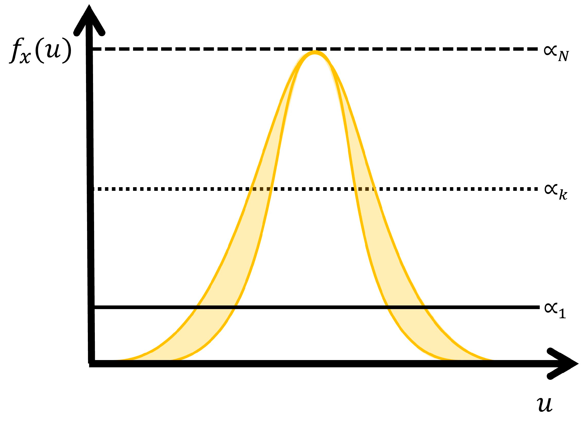
Figure 3.
Uncertainty of secondary membership grade in EWH IT3 system.
Figure 3.
Uncertainty of secondary membership grade in EWH IT3 system.
Figure 4.
Uncertainty of secondary membership grade in EWH GT2 equivalent to EWH IT3 systems.
Figure 4.
Uncertainty of secondary membership grade in EWH GT2 equivalent to EWH IT3 systems.
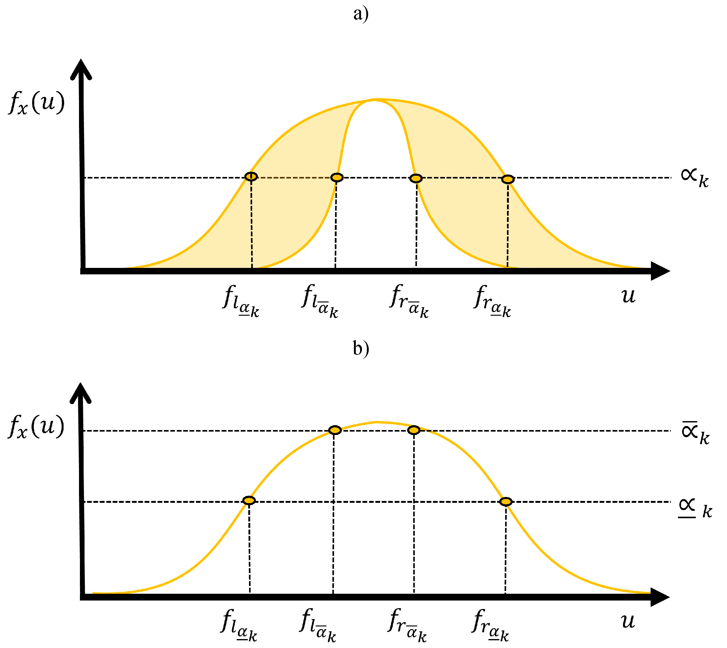
Figure 5.
Geometrical view used to calculate, a) For each level-, each -cut point of the firing interval of the antecedent section of the proposed EWH IT3 NSFLS-1 systems, and b) Its equivalent geometrical view in GT2 systems.
Figure 5.
Geometrical view used to calculate, a) For each level-, each -cut point of the firing interval of the antecedent section of the proposed EWH IT3 NSFLS-1 systems, and b) Its equivalent geometrical view in GT2 systems.
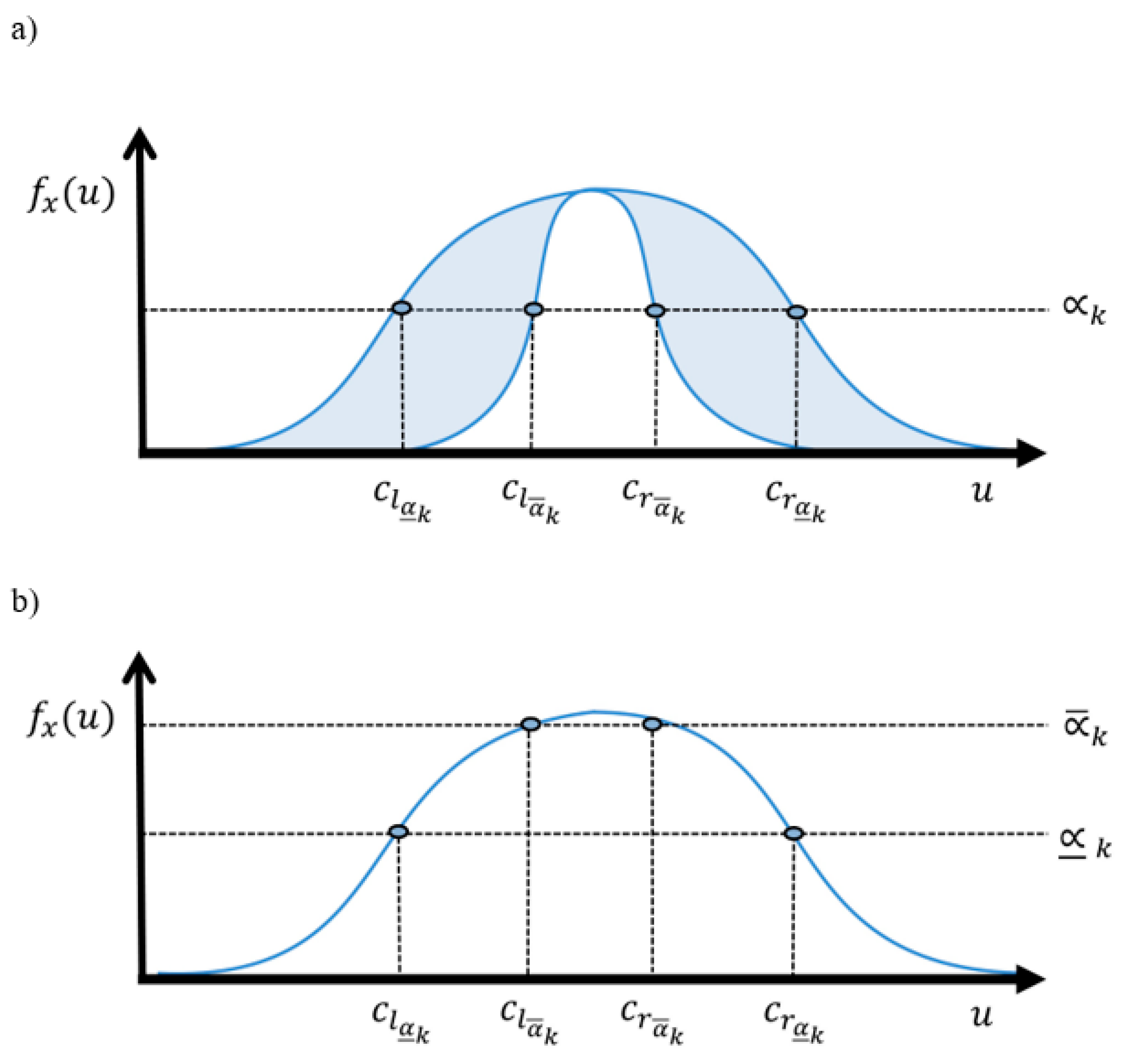
Figure 6.
Geometrical view used to calculate, a) For each level-, each -cut point of the Centroids of the consequent section of the proposed EWH IT3 NSFLS-1 system, and b) its equivalent geometrical view in GT2 systems.
Figure 6.
Geometrical view used to calculate, a) For each level-, each -cut point of the Centroids of the consequent section of the proposed EWH IT3 NSFLS-1 system, and b) its equivalent geometrical view in GT2 systems.
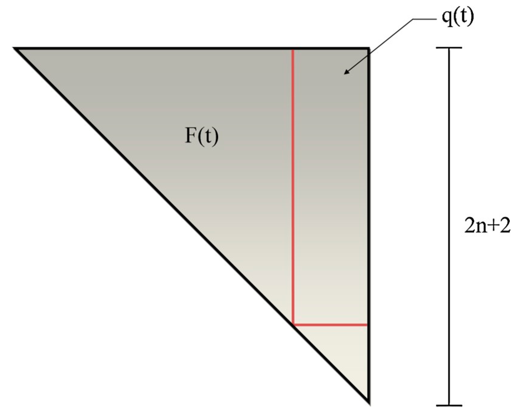
Figure 7.
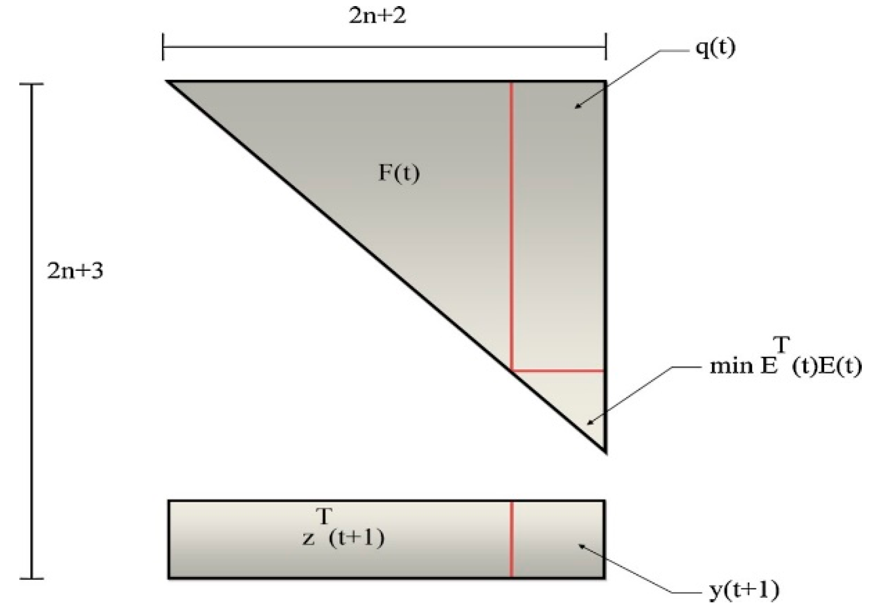
Schematic representation of
F(t) and
q(t), [
125].
Figure 7.
Schematic representation of
F(t) and
q(t), [
125].
Figure 8.
T (t+1), [
125].
Figure 8.
T (t+1), [
125].
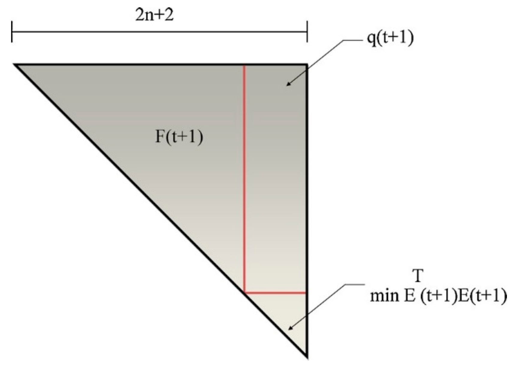
Figure 9.
Schematic representation of F
(t+1
) and q
(t+1
), [
125].
Figure 9.
Schematic representation of F
(t+1
) and q
(t+1
), [
125].
Figure 10.
Figure 10. Schematic representation of HSM, [
5].
Figure 10.
Figure 10. Schematic representation of HSM, [
5].
Figure 11.
RMSE of prediction of GT2 systems with BP-BP learning.
Figure 11.
RMSE of prediction of GT2 systems with BP-BP learning.
Figure 12.
RMSE of prediction of IT3 systems with BP-BP learning.
Figure 12.
RMSE of prediction of IT3 systems with BP-BP learning.
Figure 13.
RMSE of prediction of GT2 systems with BP-BP learning.
Figure 13.
RMSE of prediction of GT2 systems with BP-BP learning.
Figure 14.
RMSE of prediction of IT3 systems with BP-BP learning.
Figure 14.
RMSE of prediction of IT3 systems with BP-BP learning.
Figure 15.
RMSE of prediction of GT2 systems with OLS-BP learning.
Figure 15.
RMSE of prediction of GT2 systems with OLS-BP learning.
Figure 16.
RMSE of prediction of IT3 systems with OLS-BP learning.
Figure 16.
RMSE of prediction of IT3 systems with OLS-BP learning.
Figure 18.
RMSE of prediction of IT3 systems with OLS-BP learning.
Figure 18.
RMSE of prediction of IT3 systems with OLS-BP learning.
Figure 19.
RMSE of prediction of GT2 systems with OLS-BP learning.
Figure 19.
RMSE of prediction of GT2 systems with OLS-BP learning.
Figure 20.
RMSE of prediction of IT3 systems with OLS-BP learning.
Figure 20.
RMSE of prediction of IT3 systems with OLS-BP learning.
Table 1.
Difficulties of GT2 model adapted from [
41].
Table 1.
Difficulties of GT2 model adapted from [
41].
| Difficulties |
References |
| Implementation |
[42] |
| Use in practice |
[42] |
| Information is non-functional |
[43] |
| Information is un useful |
[43] |
| Information not needed |
[43] |
| Complex learning process |
[44,45,46,47,48] |
| Hard computation |
[44,47,48,49,50,51] |
| Defuzzification very complex |
[44,51,52] |
| Exhaustive computational time |
[44,47,48,49,50,51] |
| Impractical to usage |
[44] |
| Method iterative and algorithmic |
[53] |
| Determination of the number of levels- |
[49] |
Table 2.
Survey of techniques used to train the GT2 FLS models.
Table 2.
Survey of techniques used to train the GT2 FLS models.
| R |
GT2 |
Optimization model |
Knowledge acquisition
Designation |
System designation |
| S |
N |
L |
T |
A |
U |
GT2 |
Generalized type-2 |
Shadowed type-2 |
| [15] |
|
X |
TW, robustness analysis |
|
X |
|
|
|
|
X |
| [44] |
X |
|
Ordered weighted averaging (OWA) |
X |
|
|
X |
X |
|
|
| [45] |
X |
|
Data-driven |
|
|
X |
|
X |
|
|
| [47] |
|
|
Kalman Filters |
X |
|
X |
|
X |
|
|
| [48] |
X |
|
Artificial Neural Networks |
|
|
X |
|
X |
|
|
| [52] |
X |
|
Recursive Least Squares (RLS), Gradient-based Method, hybrid ANN to optimize clustering |
X |
|
|
|
X |
|
|
| [55] |
|
X |
Social spider optimization |
|
|
|
X |
X |
|
|
| [58] |
|
|
Particle Swarm Optimization (PSO) |
|
|
X |
|
X |
|
|
| [60] |
X |
|
Biogeography-Based Optimization (BBO) |
X |
|
|
|
X |
|
|
| [64] |
X |
|
Least Square Estimator (LSE), Teaching Learning Based Optimization (TLBO) |
|
|
X |
|
X |
|
|
| [72] |
|
|
Searching algorithms |
X |
X |
|
|
X |
|
|
| [73] |
X |
X |
Ant lion optimizer |
|
|
|
X |
X |
|
X |
| [79] |
X |
|
Hybrid Differential Evolution Algorithm |
|
|
X |
|
X |
|
|
| [82] |
|
X |
Harmony search |
|
|
X |
|
|
X |
X |
| [83] |
|
X |
SVM, Decision trees, ANN, Bagging and boosting, bagging, boosting, GD, fuzzy entropy, PSO, |
X |
X |
X |
X |
|
|
X |
| [84] |
|
X |
Backpropagation algorithms and RLS |
X |
|
X |
|
|
X |
|
| [85] |
|
X |
Lyapunov function |
X |
X |
X |
|
X |
X |
|
| [86] |
|
X |
Kernel ridge regression (KRR) |
X |
|
|
|
|
X |
|
| [87] |
|
X |
Hierarchically stacked though, gradient descent (GD), gaussian kernel, support vector machine (GSVM) |
X |
X |
X |
|
|
X |
|
| [88] |
|
X |
Multi-objective optimization. |
X |
|
|
|
X |
|
|
| [90] |
|
X |
Tuning laws (TW) |
X |
X |
X |
|
X |
|
|
Table 3.
IT3 FLS systems.
Table 3.
IT3 FLS systems.
| Ref. |
IT3 System |
Learning
Algorithm |
Knowledge acquisition
designation |
| S |
N-1 |
N-2 |
Hybrid |
L |
A |
U |
T |
| [1] |
X |
|
|
Classification system does not show a learning algorithm or does not need it |
|
X |
X |
|
X |
| [2] |
X |
|
|
Theoretical proposal for modelling and compare the IT3 and IT2 systems do not show the use of learning |
X |
X |
X |
|
X |
| [4] |
X |
|
|
Differential evolution |
|
X |
X |
|
X |
| [5] |
|
|
X |
Gradient descend |
X |
X |
X |
X |
X |
| [7] |
X |
|
|
Empirical knowledge of experts combined with a trial-and-error approach |
|
X |
X |
|
X |
| [8] |
X |
|
|
Fractal dimensions |
|
X |
X |
|
X |
| [9] |
X |
|
|
Statistical measures, fuzzy c-means clustering and granular computing using to construct the model not for learning |
|
|
|
X |
|
| [11] |
X |
|
|
Response aggregation |
|
X |
X |
|
X |
| [12] |
X |
|
|
Backpropagation with momentum learning |
|
X |
X |
|
X |
| [13] |
X |
|
|
Specific adaptation law |
|
X |
X |
|
X |
| [14] |
X |
|
|
Fractional-order model based on restricted Boltzmann machine (RBM) and deep learning contrastive divergence (CD) |
|
X |
|
|
X |
| [15] |
X |
|
|
Pitch adjustment rate (PArate) parameter in the original harmony search algorithm (HS) |
|
X |
|
|
X |
| [18] |
|
X |
|
Upper bound of approximate
error (AE) |
|
|
|
|
|
| [19] |
|
X |
|
Fractional order |
|
X |
|
|
X |
| [22] |
X |
|
|
Fuzzy c-regression model clustering algorithm |
|
|
X |
|
X |
| [25] |
X |
|
|
Deep reinforcement learning (DRL) |
|
X |
|
|
X |
| [26] |
X |
|
|
Unscented Kalman filter (CUKF) |
X |
X |
X |
X |
X |
| [27] |
X |
|
|
Surge-guided line-of-sight (SGLOS) and auxiliary dynamics |
|
X |
X |
|
X |
| [28] |
|
X |
|
Maximum correntropy (MC)
Unscented Kalman filter (UKF) |
|
X |
X |
|
X |
| [33] |
X |
|
|
Specific control law |
|
X |
|
|
|
| [39] |
X |
|
|
Kalman filter (UKF) |
|
X |
|
|
|
| [40] |
|
X |
|
Lyapunov adaptation rules |
|
|
X |
|
X |
| [92] |
X |
|
|
Hybrid Learning ARIMA LSTM LSTM |
X |
X |
|
|
|
| [93] |
X |
|
|
Robust adaptive command-filtered backstepping control scheme, adaptive laws |
X |
X |
|
|
|
| [94] |
X |
|
|
This is a survey, not a theoretical paper and not an application or development |
|
X |
X |
|
X |
| [96] |
X |
|
|
Bacterial foraging optimization algorithm |
|
X |
|
|
X |
| [97] |
X |
|
|
Do not have learning is a classification model |
|
X |
|
|
X |
| [98] |
X |
|
|
Spherical Fuzzy MARCOS MCGDM |
|
X |
|
|
X |
| [99] |
X |
|
|
Weighted least square (WLS) |
|
|
|
|
X |
| [100] |
X |
|
|
Actor-critic learning control algorithm and associated with Lyapunov stability examination |
|
X |
X |
|
X |
| [101] |
X |
|
|
+Nonlinear model predictive control (NMPC) |
|
X |
|
|
X |
| [102] |
X |
|
|
+Marine predator |
|
X |
X |
X |
X |
| [103] |
X |
|
|
+Maximum power point tracking (MPPT), genetic algorithm |
|
|
|
|
X |
| [104] |
X |
|
|
+Differential evolution |
|
|
X |
|
X |
| [105] |
X |
|
|
+Harmony search |
|
X |
X |
|
|
| [106] |
X |
|
|
+Harmony search and the differential evolution |
|
X |
X |
|
|
| [107] |
X |
|
|
Not learning algorithm, the parameters are changed manually |
|
X |
X |
|
|
| [108] |
X |
|
|
Terminal sliding mode controller |
|
X |
X |
|
|
| [109] |
X |
|
|
Adaptive sliding mode disturbance observer, adaptive laws, an output with continuous-time linear systems. |
X |
X |
X |
|
|
| [110] |
X |
|
|
Retained region approach (granulation) |
|
X |
X |
|
|
| [111] |
X |
|
|
Multi-objective Artificial Hummingbird Algorithm (MOAHA) |
|
X |
|
X |
|
| [112] |
X |
|
|
Enhanced Kalman filter (EKF) |
|
|
|
X |
|
| [113] |
X |
|
|
*Survey of methods is not an application |
|
X |
|
|
|
| [114] |
X |
|
|
Extended state space model-based constrained predictive functional control |
|
X |
|
|
|
| [115] |
X |
|
|
+ Event-triggered control law |
|
X |
|
|
|
| [116] |
X |
|
|
+ Cartograms to visualize both the expansion and spread |
|
X |
|
|
|
| [117] |
X |
|
|
+ Non-linear time series |
|
X |
|
|
|
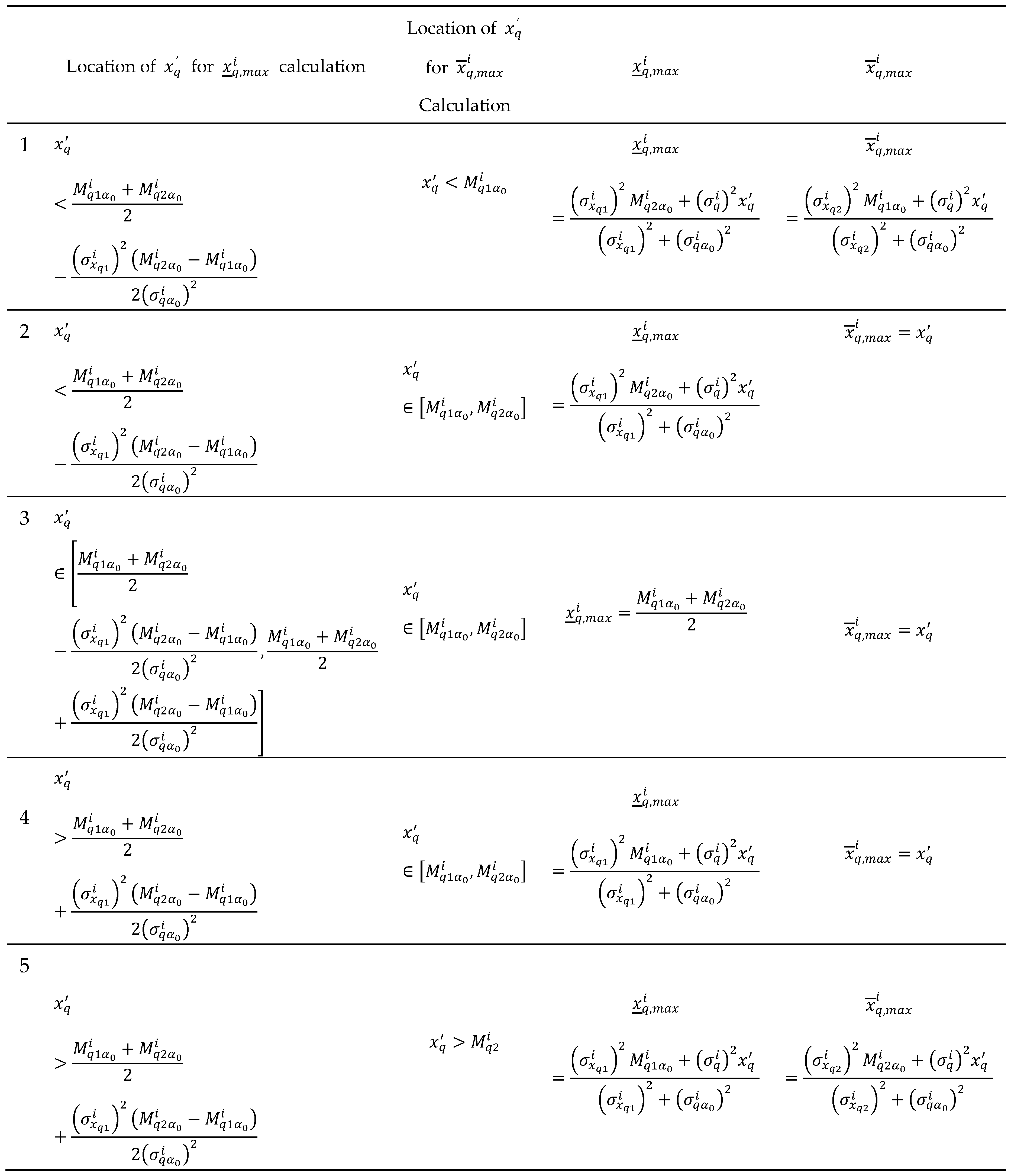
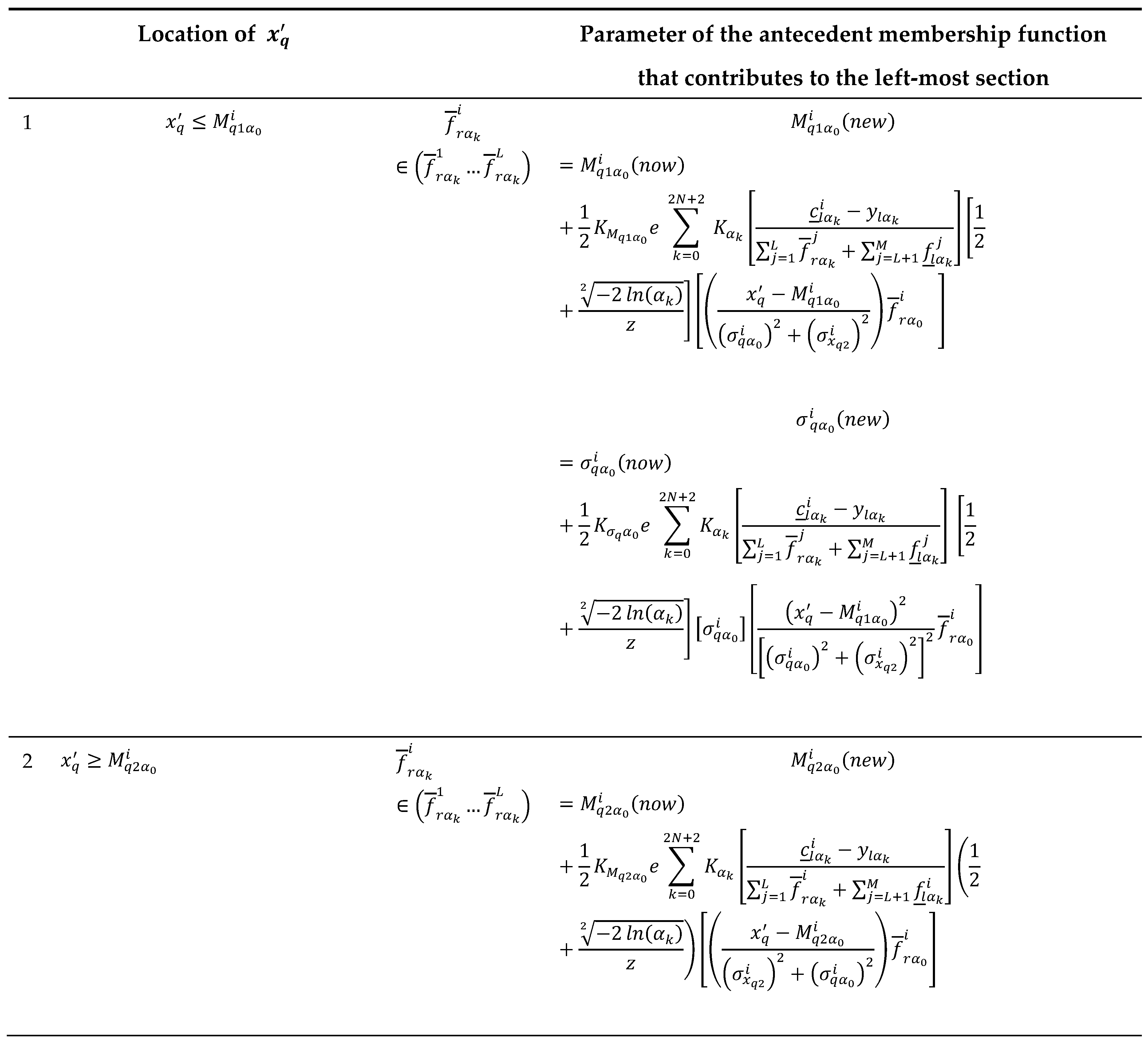
Table 4.
Locations of , for and estimation used to calculate and .
Table 4.
Locations of , for and estimation used to calculate and .
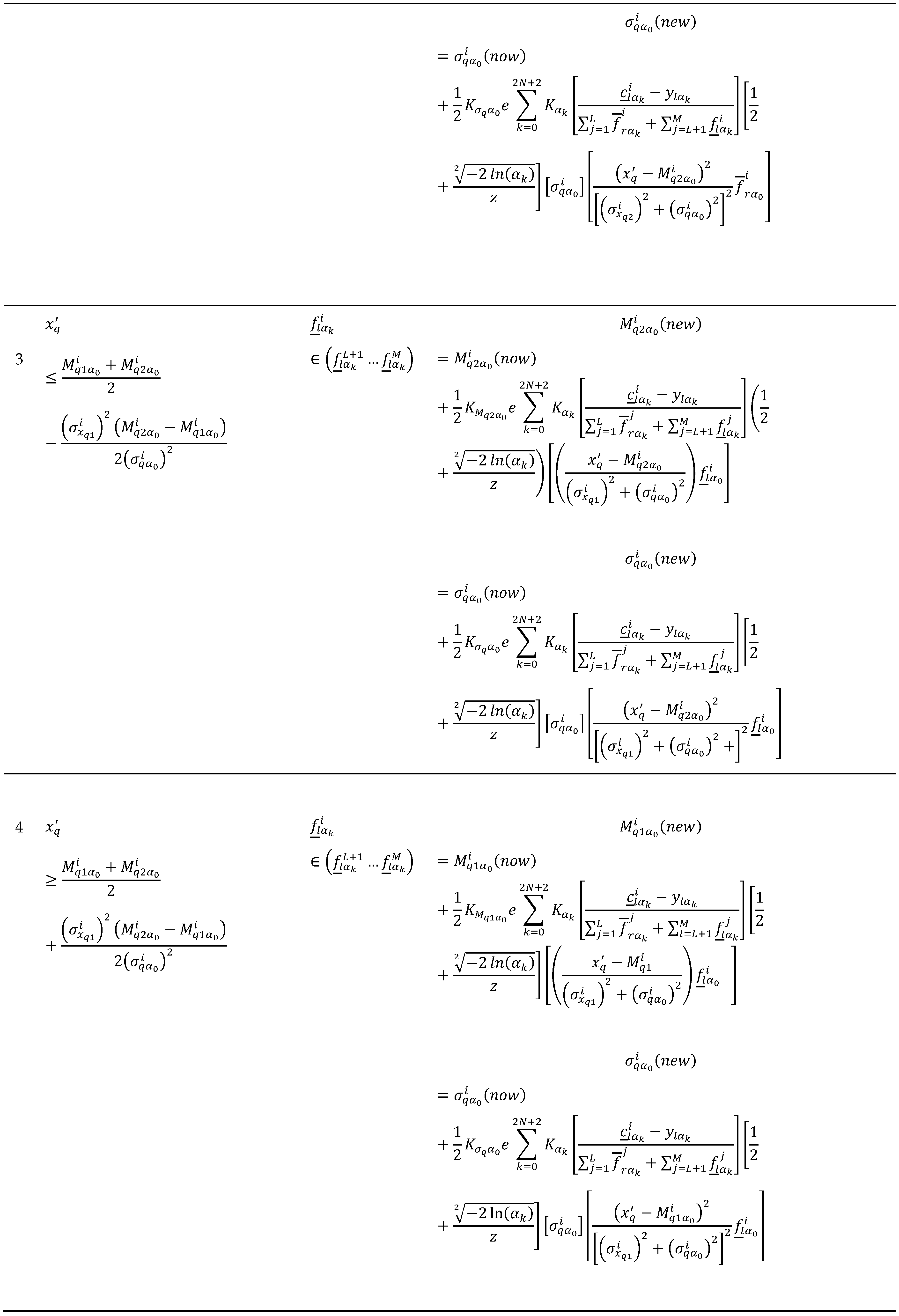
Table 5.
Gradient descent equations for antecedent training under contribution.
Table 5.
Gradient descent equations for antecedent training under contribution.
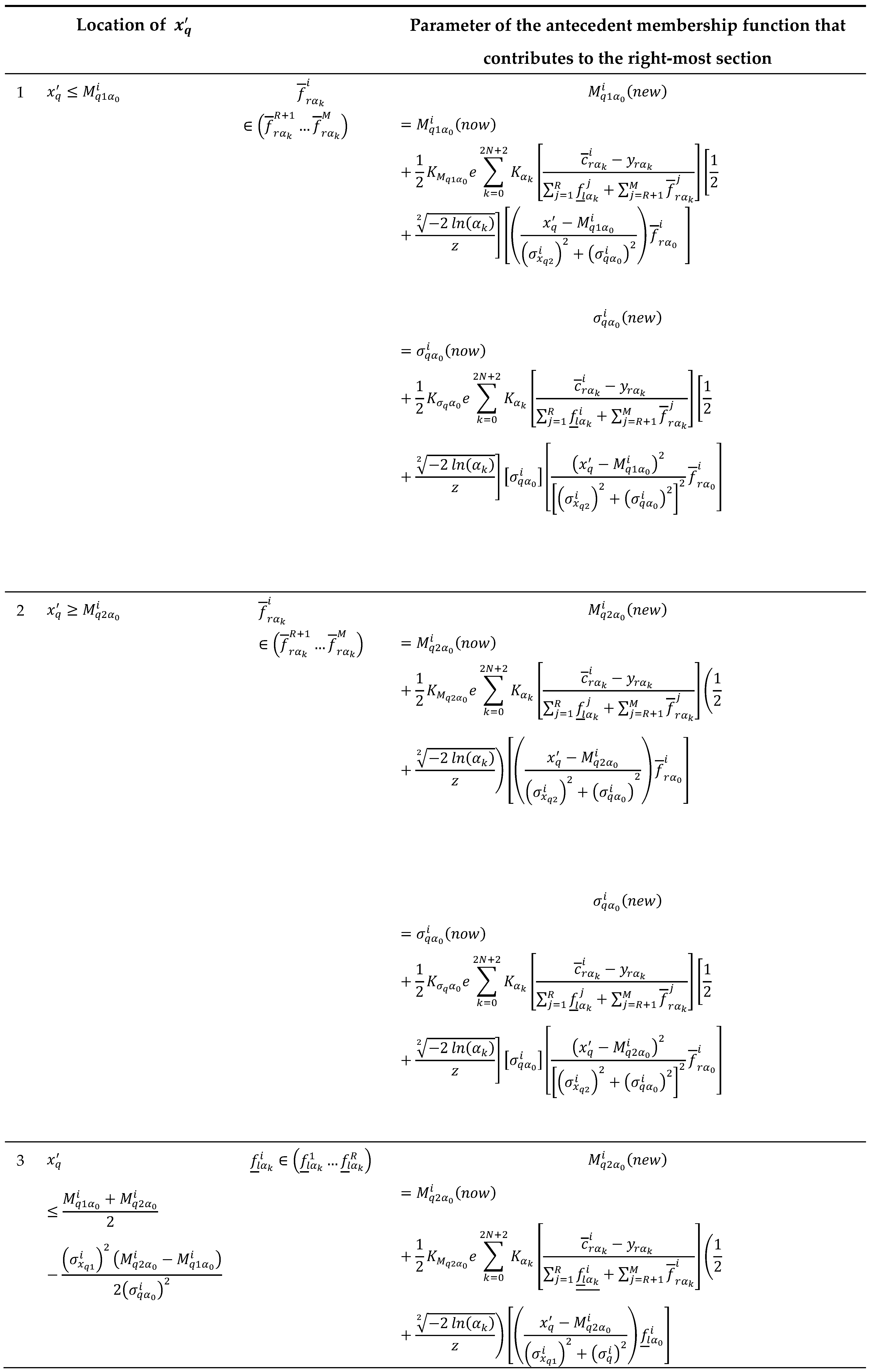
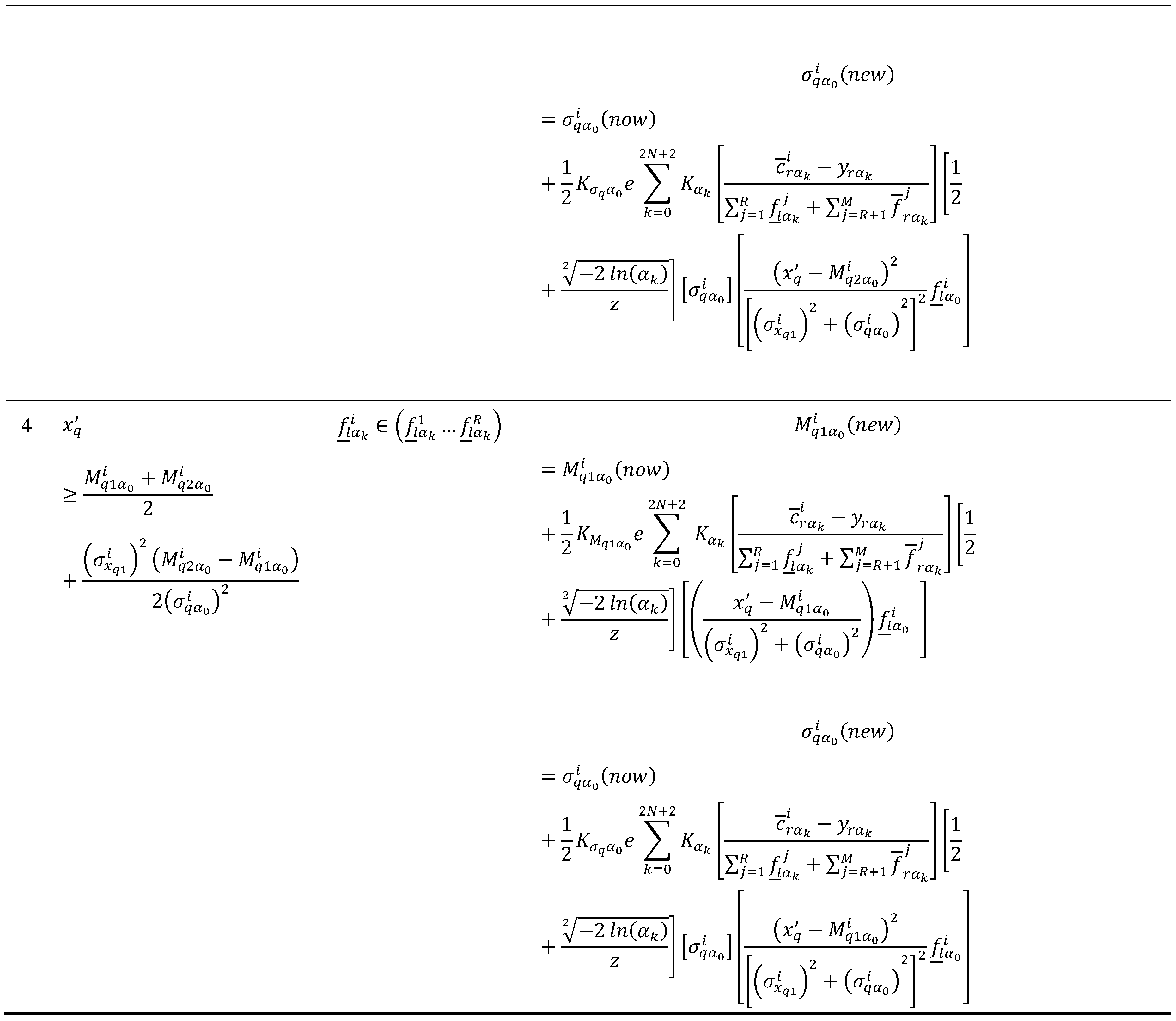
Table 6.
Gradient descent equations for antecedent training under
Table 6.
Gradient descent equations for antecedent training under
Table 7.
Type of coils.
| Coil type |
Target gage (mm) |
Target width (mm) |
Steel grade (SAE-AISI) |
| A |
1.879 |
1041.0 |
1006 |
| B |
2.006 |
991.0 |
1006 |
| C |
2.159 |
952.0 |
1006 |
Table 8.
Parameters for MFs of .
Table 8.
Parameters for MFs of .
| |
|
|
|
| 1 |
1010 |
1012 |
30 |
| 2 |
1040 |
1042 |
30 |
| 3 |
1070 |
1072 |
30 |
| 4 |
1100 |
1102 |
30 |
| 5 |
1130 |
1132 |
30 |
Table 9.
Parameters for MFs of .
Table 9.
Parameters for MFs of .
| |
|
|
|
| 1 |
32.16 |
32.66 |
2.72 |
| 2 |
34.88 |
35.38 |
2.72 |
| 3 |
37.60 |
38.10 |
2.72 |
| 4 |
40.32 |
40.82 |
2.72 |
| 5 |
43.04 |
43.54 |
2.72 |
Table 10.
Initial fuzzy rule base.
Table 10.
Initial fuzzy rule base.
| Rule |
|
|
|
|
|
|
|
|
| 1 |
1010 |
1012 |
30 |
32.16 |
32.66 |
2.7 |
960 |
962 |
| 2 |
1010 |
1012 |
30 |
34.88 |
35.38 |
2.7 |
958 |
960 |
| 3 |
1010 |
1012 |
30 |
37.60 |
38.10 |
2.7 |
956 |
958 |
| 4 |
1010 |
1012 |
30 |
40.32 |
40.82 |
2.7 |
954 |
956 |
| 5 |
1010 |
1012 |
30 |
43.04 |
43.54 |
2.7 |
952 |
954 |
| 6 |
1040 |
1042 |
30 |
32.16 |
32.66 |
2.7 |
970 |
972 |
| 7 |
1040 |
1042 |
30 |
34.88 |
35.38 |
2.7 |
968 |
970 |
| 8 |
1040 |
1042 |
30 |
37.60 |
38.10 |
2.7 |
966 |
968 |
| 9 |
1040 |
1042 |
30 |
40.32 |
40.82 |
2.7 |
964 |
966 |
| 10 |
1040 |
1042 |
30 |
43.04 |
43.54 |
2.7 |
962 |
964 |
| 11 |
1070 |
1072 |
30 |
32.16 |
32.66 |
2.7 |
980 |
982 |
| 12 |
1070 |
1072 |
30 |
34.88 |
35.38 |
2.7 |
978 |
980 |
| 13 |
1070 |
1072 |
30 |
37.60 |
38.10 |
2.7 |
976 |
978 |
| 14 |
1070 |
1072 |
30 |
40.32 |
40.82 |
2.7 |
974 |
976 |
| 15 |
1070 |
1072 |
30 |
43.04 |
43.54 |
2.7 |
972 |
974 |
| 16 |
1100 |
1102 |
30 |
32.16 |
32.66 |
2.7 |
990 |
992 |
| 17 |
1100 |
1102 |
30 |
34.88 |
35.38 |
2.7 |
988 |
990 |
| 18 |
1100 |
1102 |
30 |
37.60 |
38.10 |
2.7 |
986 |
988 |
| 19 |
1100 |
1102 |
30 |
40.32 |
40.82 |
2.7 |
984 |
986 |
| 20 |
1100 |
1102 |
30 |
43.04 |
43.54 |
2.7 |
982 |
984 |
| 21 |
1130 |
1132 |
30 |
32.16 |
32.66 |
2.7 |
1000 |
1002 |
| 22 |
1130 |
1132 |
30 |
34.88 |
35.38 |
2.7 |
998 |
1000 |
| 23 |
1130 |
1132 |
30 |
37.60 |
38.10 |
2.7 |
996 |
998 |
| 24 |
1130 |
1132 |
30 |
40.32 |
40.82 |
2.7 |
994 |
996 |
| 25 |
1130 |
1132 |
30 |
43.04 |
43.54 |
2.7 |
992 |
994 |
Table 11.
Comparison between the benchmark models (IT2 SFLS and IT2 NSFLS-1) and GT2 models with BP-BP learning using the classic WH algorithm and the EWH algorithm.
Table 11.
Comparison between the benchmark models (IT2 SFLS and IT2 NSFLS-1) and GT2 models with BP-BP learning using the classic WH algorithm and the EWH algorithm.
|
-cuts |
1 |
| IT2 SFLS |
1.4249 |
| IT2 NSFLS-1 |
1.2542 |
| WH GT2 SFLS (BP-BP) |
1.4515 |
| EWH GT2 SFLS (BP-BP) |
1.4497 |
| WH GT2 NSFLS-1 (BP-BP) |
1.0383 |
| EWH GT2 NSFLS-1 (BP-BP) |
1.0383 |
Table 12.
Comparison between the benchmark models (IT2 SFLS and IT2 NSFLS-1) and IT3 models with BP-BP learning using the classic WH algorithm and the EWH algorithm.
Table 12.
Comparison between the benchmark models (IT2 SFLS and IT2 NSFLS-1) and IT3 models with BP-BP learning using the classic WH algorithm and the EWH algorithm.
|
-cuts |
1 |
2 |
| IT2 SFLS |
1.4249 |
|
| IT2 NSFLS-1 |
1.2542 |
|
| WH IT3 SFLS (BP-BP) |
|
1.4212 |
| EWH IT3 SFLS (BP-BP) |
|
1.4192 |
| WH IT3 NSFLS-1 (BP-BP) |
|
0.9729 |
| EWH IT3 NSFLS-1 (BP-BP) |
|
0.8761 |
Table 13.
Comparison between the benchmark models (IT2 SFLS and IT2 NSFLS-1) and GT2 models with BP-BP learning using the classic WH algorithm and the EWH algorithm with different number of -cuts.
Table 13.
Comparison between the benchmark models (IT2 SFLS and IT2 NSFLS-1) and GT2 models with BP-BP learning using the classic WH algorithm and the EWH algorithm with different number of -cuts.
|
-cuts |
1 |
10 |
100 |
1000 |
| IT2 SFLS |
1.4249 |
|
|
|
| IT2 NSFLS-1 |
1.2542 |
|
|
|
| WH GT2 SFLS (BP-BP) |
1.4515 |
1.1501 |
1.4912 |
1.5727 |
| EWH GT2 SFLS (BP-BP) |
1.4497 |
1.1433 |
1.4852 |
1.5166 |
| WH GT2 NSFLS-1 (BP-BP) |
1.0397 |
1.2338 |
1.097 |
1.3325 |
| EWH GT2 NSFLS-1 (BP-BP) |
1.0383 |
1.1534 |
1.0321 |
1.326 |
Table 15.
Comparison between the benchmark models (IT2 SFLS and IT2 NSFLS-1) and GT2 models with OLS-BP learning using the classic WH algorithm and the EWH algorithm.
Table 15.
Comparison between the benchmark models (IT2 SFLS and IT2 NSFLS-1) and GT2 models with OLS-BP learning using the classic WH algorithm and the EWH algorithm.
|
-cuts |
1 |
| IT2 SFLS |
1.4249 |
| IT2 NSFLS-1 |
1.2542 |
| WH GT2 SFLS (OLS-BP) |
0.9389 |
| EWH GT2 SFLS (OLS-BP) |
0.9424 |
| WH GT2 NSFLS-1 (OLS-BP) |
0.8952 |
| EWH GT2 NSFLS-1 (OLS-BP) |
0.8724 |
Table 16.
Comparison between the benchmark models (IT2 SFLS and IT2 NSFLS-1) and IT3 models with OLS-BP learning using the classic WH algorithm and the EWH algorithm.
Table 16.
Comparison between the benchmark models (IT2 SFLS and IT2 NSFLS-1) and IT3 models with OLS-BP learning using the classic WH algorithm and the EWH algorithm.
|
-cuts |
1 |
2 |
| IT2 SFLS |
1.4249 |
|
| IT2 NSFLS-1 |
1.2542 |
|
| WH IT3 SFLS (OLS-BP) |
|
0.9389 |
| EWH IT3 SFLS (OLS-BP) |
|
0.9424 |
| WH IT3 NSFLS-1 (OLS-BP) |
|
0.8952 |
| EWH IT3 NSFLS-1 (OLS-BP) |
|
0.8724 |
Table 17.
Comparison between the benchmark models (IT2 SFLS and IT2 NSFLS-1) and GT2 models with OLS-BP learning using the classic WH algorithm and the EWH algorithm.
Table 17.
Comparison between the benchmark models (IT2 SFLS and IT2 NSFLS-1) and GT2 models with OLS-BP learning using the classic WH algorithm and the EWH algorithm.
|
-cuts |
1 |
10 |
100 |
1000 |
| IT2 SFLS |
1.4249 |
|
|
|
| IT2 NSFLS-1 |
1.2542 |
|
|
|
| WH GT2 SFLS (OLS-BP) |
0.9424 |
0.9332 |
0.9356 |
0.9631 |
| EWH GT2 SFLS (OLS-BP) |
0.9521 |
0.9438 |
0.9458 |
0.9658 |
| WH GT2 NSFLS-1 (OLS-BP) |
0.8979 |
0.9316 |
0.8888 |
1.002 |
| EWH GT2 NSFLS1 (OLS-BP) |
0.8851 |
0.9183 |
0.8659 |
0.9967 |
Table 18.
Comparison between the benchmark models (IT2 SFLS and IT2 NSFLS-1) and IT3 models with OLS-BP learning using the classic WH algorithm and the EWH algorithm.
Table 18.
Comparison between the benchmark models (IT2 SFLS and IT2 NSFLS-1) and IT3 models with OLS-BP learning using the classic WH algorithm and the EWH algorithm.
|
-cuts |
1 |
2 |
10 |
100 |
1000 |
| IT2 SFLS |
1.4249 |
|
|
|
|
| IT2 NSFLS-1 |
1.2542 |
|
|
|
|
| WH IT3 SFLS (OLS-BP) |
|
0.9389 |
0.9247 |
0.9177 |
0.9461 |
| EWH IT3 SFLS (OLS-BP) |
|
0.9424 |
0.9184 |
0.9231 |
0.9556 |
| WH IT3 NSFLS-1 (OLS-BP) |
|
0.8952 |
0.9127 |
0.8795 |
0.9666 |
| EWH IT3 NSFLS-1 (OLS-BP) |
|
0.8724 |
0.8905 |
0.8634 |
0.9408 |

