1. Introduction
Numerical integration is a technique often used in a wide variety of fields, ranging from the fundamental sciences to medicine [
1] and the financial world [
2,
3,
4]. For classical computers, many algorithms exist, but these algorithms have their limitations. In this paper, the promising algorithm of [
5] for a quantum computer is used to provide an estimate of the future performance of this technique compared to classical solutions.
The problem of integration is given by
where
p may be the measure or some probability density function against which the function
f is integrated. Although many integration techniques exist, many functions remain impossible to integrate exactly. Numerical integration techniques are needed for those. However, many of these techniques suffer from dimensionality problems. If the run-time of a numerical integration algorithm increases exponentially with the dimension of the integration domain, this algorithm will soon face it limitations [
6,
7].
For such high dimensional problems on classical computers Monte Carlo integration (MCI) is an effective method. In Monte Carlo integration a random sample from the integration domain is chosen and its function value is determined. The average function value over all samples multiplied by the volume of the domain gives an estimate of the integral [
8]. Since the function is evaluated once for each sample point, the number of function evaluations
N is the same as the number of samples. The error of MCI decreases as
[
8]. If the sampling is perfectly random, this is the only source of errors and the precision is determined by the number of samples the computer can process. For related techniques, such as Quasi-Monte Carlo, the convergence rate for certain classes of functions is much faster [
9,
10].
When considering quantum computers, more options arise. One of the mostly studied algorithms for integration problems is the Quantum Amplitude Estimation algorithm [
5,
11,
12,
13,
14]. This algorithm is chosen because it is likely that it will function on near-term NISQ devices [
15]. The quantum amplitude estimation (QAE) algorithm is based on the Quantum phase estimation algorithm which is described in [
16]. A large part of this algorithm is used to perform the Fourier transform on a quantum circuit. Doing this classically, for example with maximum likelihood estimation [
5], simplifies the circuit considerably. This method is improved in the noiseless setting by [
17]. A method without post-processing is Iterative QAE [
18]. However, its algorithm has a varying execution length, depending on the desired accuracy. A generalization of these for real-valued integrands [
19] or for minimal circuit depth [
7] have also been constructed. Several of these amplitude estimation approaches can be presented in a uniform fashion [
20].
1.1. Numerical integration
The only source of error in Monte Carlo integration is the sampling error, which decreases as
with the number of samples
N. Since only a finite number of samples is taken, this error is present too in the QAE. To be more precise, in the approach used here [
5], a circuit of
qubits generates
samples. This means that QAE can only be beneficial if
, where
N is the number of MCI samples. This is certainly possible, since the number of samples on the quantum computer increases exponentially with the number of available qubits. Besides this sampling error, the quantum computer suffers from other errors inherent to the quantum process. The challenge is thus to device integration procedures for which the quantum errors decay faster than
, where
N will have to be interpreted as the number of function evaluations.
The QAE algorithm looks very promising [
21], but it is unclear how it will perform in the near future and when it will outperform classical integration methods. To answer these questions a noise metric will be introduced that can be derived from the quantum volume (QV) and from actual QAE runs. The observed exponential growth of the quantum volume can thus be translated to error parameters for QAE runs in the NISQ era. In this way, predictions for the Fisher information per second can be made. This is the metric that determines the error in numerical integration algorithms and can be approximated both for QAE and classical MCI procedures.
For this work a universal algorithm is used, meaning that the approach works for any suitable function f and probability density function p. This means that optimizations possible for specific classes of functions, such as functions with shallow implementations, cannot be applied. For such functions, the performance estimates will be too pessimistic.
1.2. Quantum Volume
The most-used metric to describe the performance of quantum computers is IBM’s quantum volume [
22]
where
N is the number of qubits of the hardware and
d is the depth of the randomized circuit that can run reliably [
22]. Such a circuit on
q qubits will return on measurement each
q-bit answer with a certain probability. By definition, half of the answers will have a probability larger than the median. These are called the heavy outputs. The idea of a QV experiment is to reproduce as many of these heavy outputs using the noisy quantum computer. Guessing would yield half of the heavy outputs, so it should be possible to improve this. IBM has defined [
22] a noisy quantum computer to run reliably, if with a one-sided
confidence the quantum circuit will retrieve at least
of the heavy outputs of a random circuit. The quantum volume of a device is then the largest square circuit, consisting of
d rounds of random permutations and pair-wise random
-matrices on
d qubits that runs reliably.
To ensure that the number of samples in numerical integration is large enough to beat classical machines the quantum computer should work on suficiently many qubits. The classical example in
Section 3.1 suggests that this should be something like
samples. For this, quantum computers with at least 27 qubits are needed, which puts a lower bound on the quantum volume required to perform competitive QAE. IBM reached a quantum volume of 512 with its Prague machine [
23], which corresponds approximately to a doubling of the quantum volume every 9 months since 2018 [
24]. Based on [
25] one would deduce that the quantum volume doubles every 4 months for Quantinuum systems since June 2020. There are estimates [
26] that the quantum volume has doubled approximately every 6 months since its conception, which is what we will use here as a forecast of the quantum volume
Here,
T is the time in months, since November 2018. Based on (
3) a reliable machine with 27 qubits requires
months, bringing us to May 2031. However, this is the situation for quantum volume circuits. The error sensitivity of quantum amplitude estimation circuits is different.
Notice that the observed exponential growth of the quantum volume is conservative in comparison with optimistic heuristics, such as the double exponential growth of Rose’s law or Neven’s law. These are based on a supposed exponential relation between the number of qubits and the equivalent number of classical bits in combination with an observed exponential growth of the number of available qubits over time [
27].
2. Materials and Methods
2.1. QAE without noise
Based on the work of [
5], the problem of numerical integration of bounded real functions against arbitrary probability distributions on a compact set is considered. The conditions of this problem may be relaxed in several ways at a later stage. The problem is given by
It is assumed that the function
f is sufficiently well-known that it is possible to produce upper and lower bounds for its extreme values. Shifting and scaling
f by them, it can be guaranteed that
, so that a
exists, such that
The probability distribution on the
q qubits is implemented by a unitary operator
The function
f uses an ancilla qubit, as it is implemented by a unitary operator
on
qubits as
It follows that
yields the desired state.
In order to run the QAE algorithm, an amplification operator is needed. This operator is defined as
. The operators
and
act trivially on other states. The (unitary) rotation operator
satisfies
. Using this it follows directly that
After
m amplification steps there are
function evaluations performed to generate the average over
samples. This means that the number of function evaluations needed for one estimate is much lower. This is what increases the efficiency of this method and constitutes the potential quantum advantage. The difference between
and
can be bounded by the law of larger number. It decreases as
. QAE can only yield better results if the number of qubits is large enough to generate more samples than current Monte Carlo techniques use.
Once the quantum circuits are executed for a set of amplification powers
, the most likely angle to explain these measurements needs to be determined. This yields the best possible answer for the integral by (
5). For each amplification power
,
measurements/shots are performed with
measurements of
. The most likely angle
to have generated these measurements is the one that maximizes the likelihood
2.2. QAE on noisy processors
The reliability of current quantum computers is reduced by various sources of noise and thus it is necessary to account for its influence [
28]. To compare the noiseless with the noisy QAE, a simple, parameterized, phenomenological noise model is introduced. Its main parameter is the probability
a that a circuit on noisy hardware will be performed and measured correctly. This means that with probability
an error occurs. In this case, it is assumed that a random output will be measured. This model is quite practical and simple to analyze. Furthermore, since the circuit of interest only measures one qubit, there is little benefit using a more sophisticated noise model.
The probability of a successfully run circuit is defined as
based on two parameters and the size
s of the circuit, decomposed in the basis gates and transpiled into the topology of the used hardware. The parameter
tries to capture the initialization and measurement errors. The parameter
describes the probability that a slice of the circuit of size 100 is performed correctly. The size of 100 gates is chosen, so that
is somewhat spread over the interval
. It is assumed that all slices are independent of each other in this respect, so that an exponentially falling success probability is obtained.
To be able to extract information out of the measurements, the parameter
must be large enough. In order to make a good estimation of the parameters of the error model, the error model itself needs to be tested. This is done by using small test circuits which can be simulated without errors. Next, the experiments are repeated on noisy quantum processors. The noiseless probabilities are denoted by
and the noisy ones by
. To determine the noise probabilities a posteriori, the best fitting error probability
a is found, such that the sum of squared errors
over the
n states is minimized. This is solved by
The ratio of
against
can be used to describe the quality of the noise model. This is the
-score
The interpretation as a probability dictates that
. Nonetheless, fluctuations in the measurement results may lead to solutions of (
12) that lie outside this interval. Outliers
are set to
and very negative values
to
. This is done to disturb the statistics of
a as little as possible.
Values of a around 1 are expected for ideal and values around 0 for noise-dominated devices. Since the latter is more common in experiments, small negative values may occur regularly as a result of statistical fluctuations. Therefore, we include these in the computations.
The QAE circuits are too extensive and deep to run on the currently available noisy hardware and are thus unsuited to test the performance of the noise model. Therefore the choice is made to make use of generated dummy circuits composed of the same gates as the circuits for the QAE amplification rounds. A circuit consists of R rounds, where in each one a number of not-gates and one multi-controlled y-rotation are performed. The rotation acts on the last qubit and is controlled by randomly selected qubits, which are all flipped to 1 and flipped backwards after the rotation. Only the last qubit will be measured. The tests are run on IBM-perth (7qubits) and the results are used to fit the noise model. The tests have also been run on IBM-guadalupe (16 qubits). These circuits for one or more amplification rounds are so large that all obtained values of a will be effectively zero.
2.3. Topologies
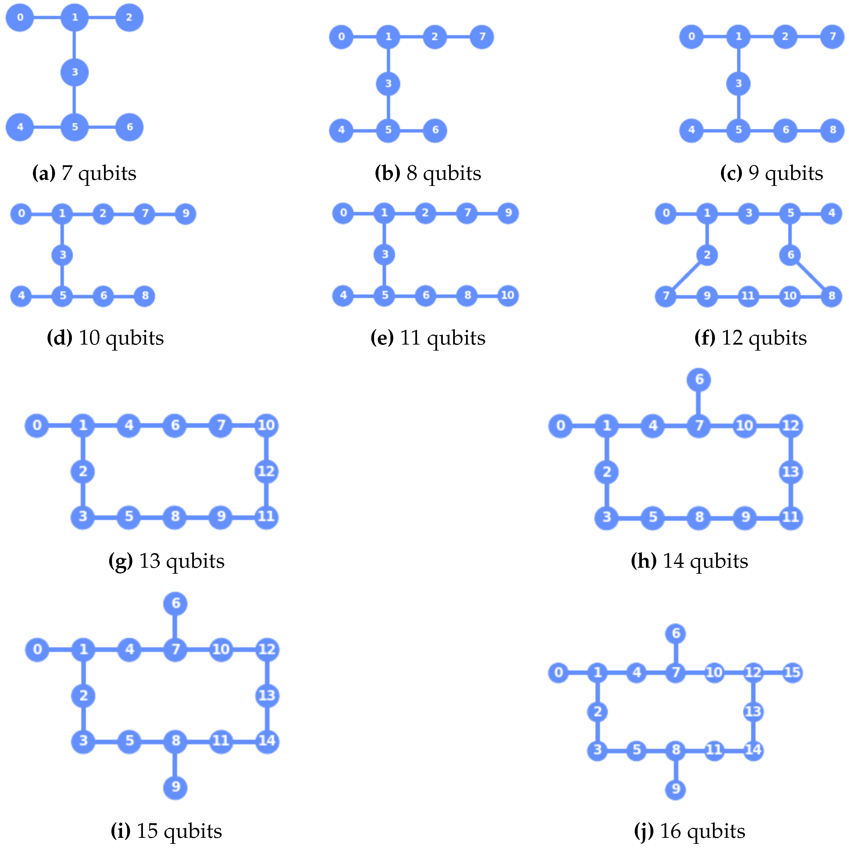
Besides IBM Perth and Guadalupe it is useful to run the circuits on quantum processors of intermediate sizes. To this end a series of topologies for 8 until 15 qubits has been drawn that should interpolate between Perth (7 qubits) and Guadalupe (16 qubits). These are shown in
Figure 1. The idea behind these choices is that the topology should not lead to outliers in the results of the experiments.
2.4. Fisher information
The amount of information generated by a numerical integration method is defined as the Fisher information. For QAE with depolarizing noise it can be derived [
28] from the noiseless case. According to the proposed noise model (
10) the noisy amplitude is measured with probability
The probability of an error occurring,
, is divided over 2 possible states. For the likelihood function per shot this implies that
From this the Fisher information can be shown [
28] to be
where
and
. In particular the value
is of interest. In this case
, so that the error parameters are irrelevant and the Fisher information is maximal. If possible, QAE problems should be formulated in such a way that the expected angle is
. The Fisher information (
15) becomes in this case
which should be maximized under the condition that
This is solved by setting
, where
maximizes
. To determine precisely when to switch from
, solve
How the choice of amplification powers depends on the a priori knowledge of
is an interesting question, but out of scope here.
3. Results
3.1. A Monte Carlo example
The interest in QAE comes from its ability to converge faster than classical Monte Carlo integration. Therefore, a simple estimate of the reference speed of classical Monte Carlo integration is useful to choose the parameters of the quantum algorithm. For this purpose the integral
with
,
and
is determined numerically with
samples. This requires
seconds on a legacy processor, estimated at 0.2 Tflops. In an operational setting, a computing cluster of 100 Tflops could thus evaluate approximately
samples per second. Classical computers work both without errors and without amplification rounds, so that the Fisher information per second is
, following (
16).
3.2. Results for the Error Model
To test the assumptions behind the noise model shallow versions of QAE circuits are run on real and simulated hardware. The results are used to fit the parameters of the noise model.
For each number of rounds circuits for multiple functions are run and measured 10001 times
1. These results are compared with those of the noiseless simulations of the same circuits. Using this information an error probability can be fitted to
to explain the difference. The quality of the model can then be expressed by the
-score, depicting the fraction of the variance in the data that is explained by the noise model. The obtained results are presented in
Table 1. It can be seen that for
rounds, only a measurement of the last qubit is performed after optimization of the circuit. This explains the depth and size of these circuits and correponds to the interpretation of the parameter
from (
10).
To test whether this noise model also works for more qubits, the procedure has been repeated for larger noisy QPU’s. This has been done using the topologies described in
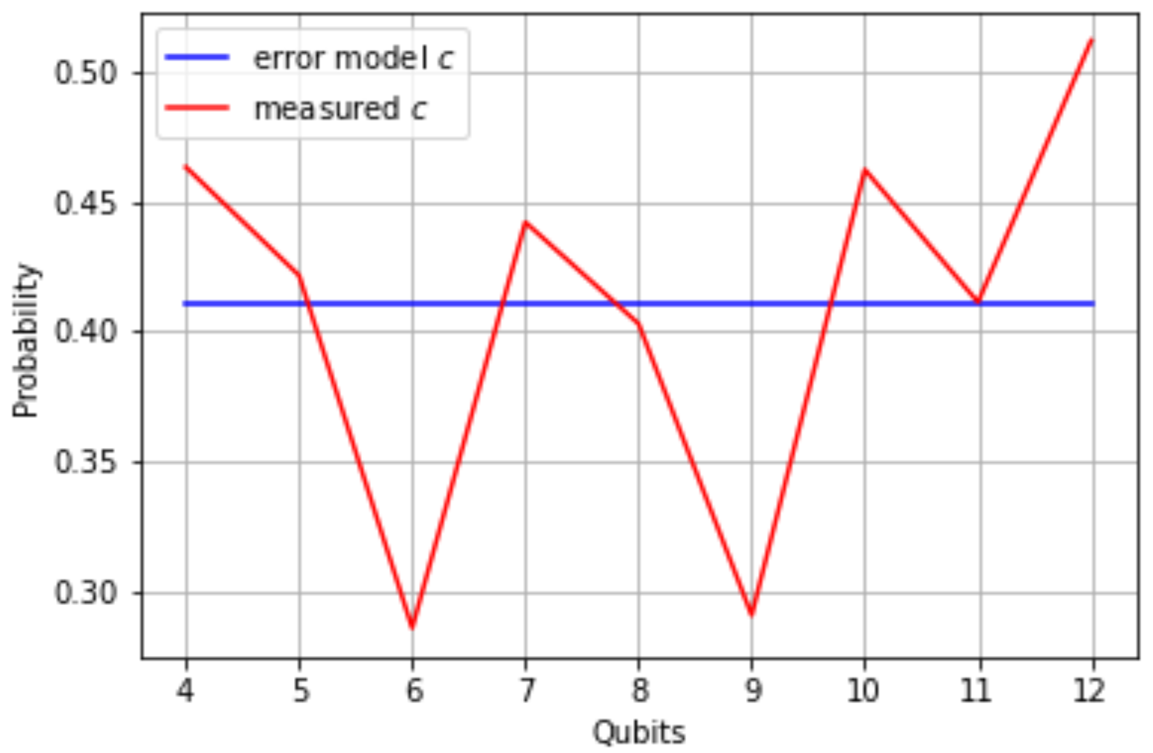
Section 2.3. Instead of a real machine with real noise, a thermal noise model has been used. This causes the difference between the values for
c in
Figure 2 and the value found in
Table 1. The simulation time for circuits with 13 - 15 qubits exceeded the available time and could not be included in
Figure 2.
The used implementation of the function and the probability distribution is universal. It is of (approximately) equal size for all sufficiently smooth functions. That the average depth and size in
Table 1 are not integers can be explained by the optimization of the circuit, when decomposing and transpiling it for the hardware.
3.3. Estimations for the size of circuits
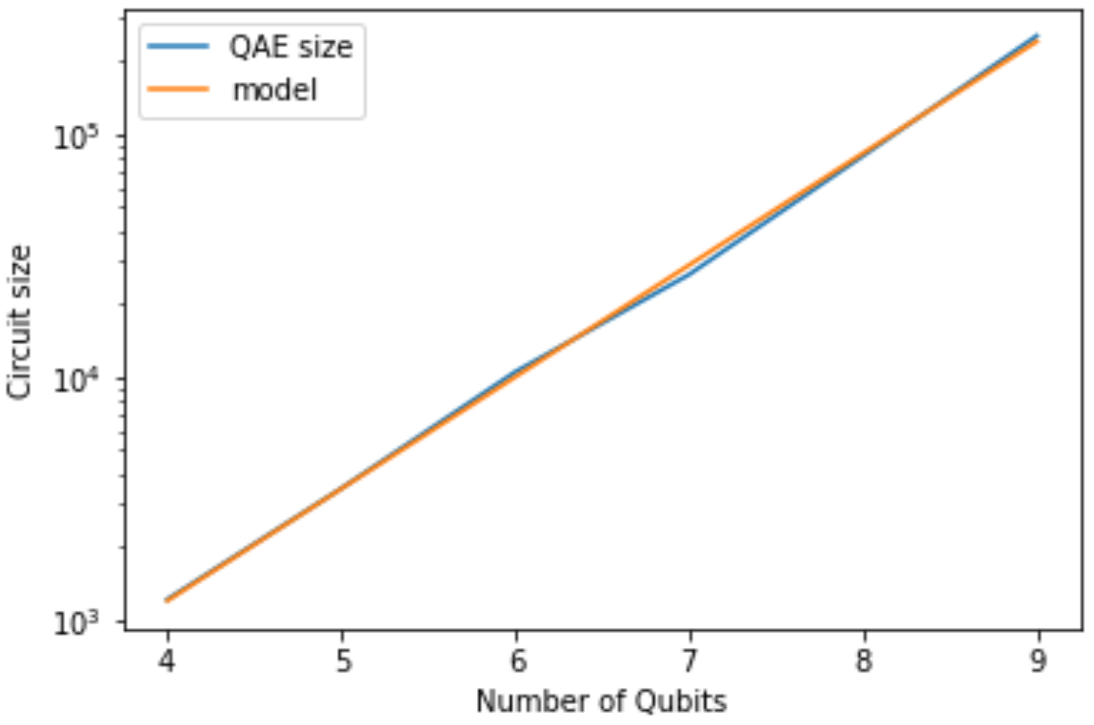
The reliability of a run on a quantum machine depends, among other things, on the size of the circuit. It is, therefore, important to describe the scaling of the size of the circuits for more qubits. For a selection of qubits circuits are build for a function
f with uniformly random function values. For each of these circuits the size is measured and the results are shown in
Figure 3.
The size
of a QAE circuit is modelled in the number of qubits
q and the number of amplification rounds
R by
where the obtained parameters are
and
. The results are also shown in
Figure 3.
A separate set of measurements has confirmed the dependence on the number of amplification rounds R. This dependence is also to be expected from the construction.
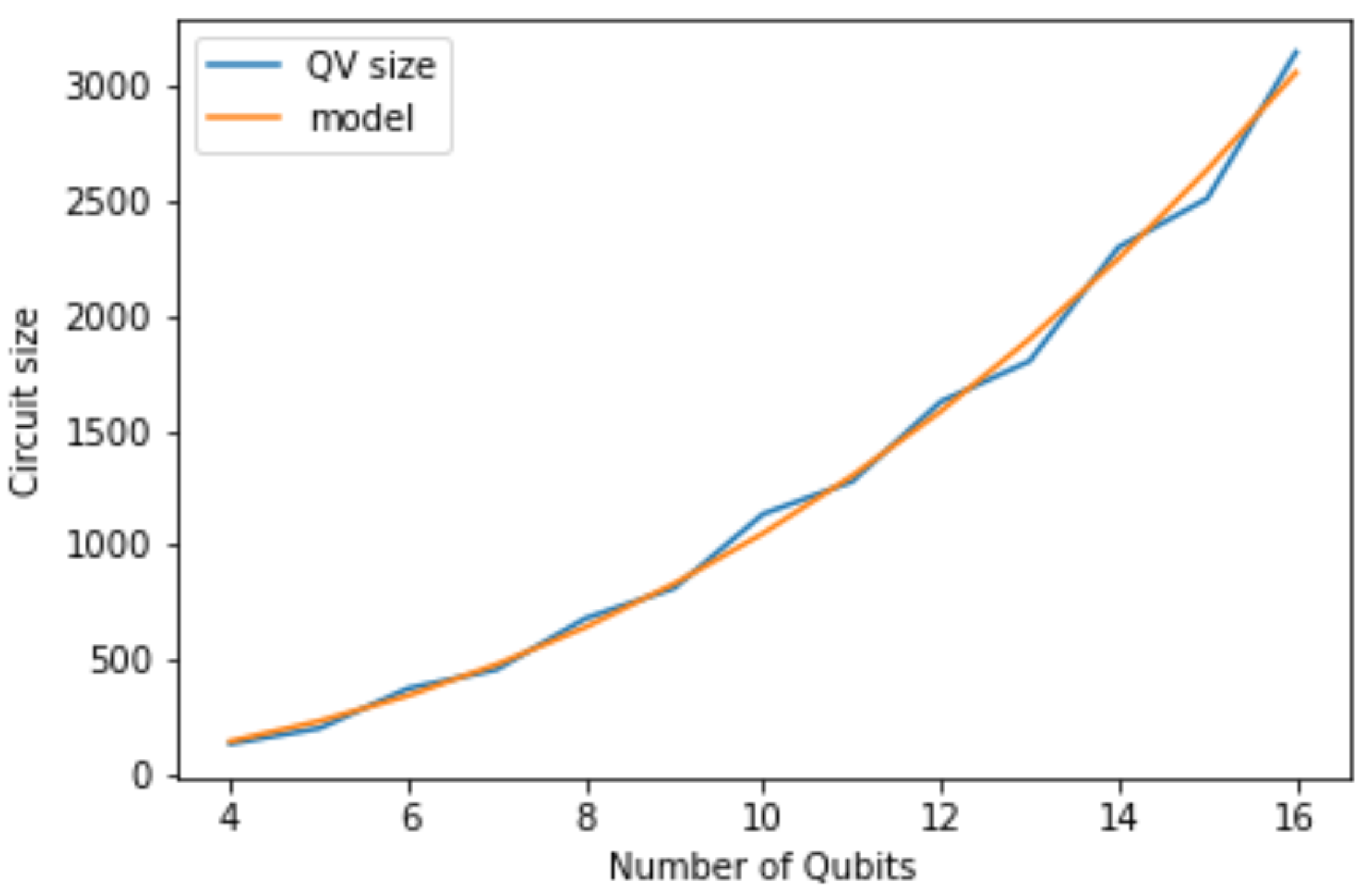
A similar exercise can be performed for the quantum volume circuits. In this case, the size of the circuit depends on the number of qubits only, since quantum volume circuits are squared. The depth is equal to the number of qubits. Because the circuits need to be transpiled, a quadratic relation between the number of qubits and the depth of the generated circuits is obtained. The results are shown in
Figure 4 and the obtained model is given by
with
being the size of the quantum volume circuit,
q the number of qubits and
and
are the fitting parameters.
3.4. Success in a quantum volume experiment
A quantum volume experiment is defined to be successful if of the heavy outputs is found with a one-sided certainty. The fraction of heavy outputs is determined by repetition of the same circuit, whereas the certainty stems from repetition of the experiment with different circuits.
In a prepared quantum volume circuit with
q rounds over
q qubits the state
is measured with probability
. The probabilities are ordered, so that
. It was shown that the exponential distribution
with
is a good approximation for these probabilities [
29], so that the probability density of finding a state with probability
p in a QV circuit is given by
.
The probability of a heavy output in one measurement is given by
where
m is the median of the exponential distribution
. In an actual experiment on a noise QPU a heavy output will be found with probability
. The variance of this measurement is then given by
. After
N measurement, the experiment has passed the test, if
This means that a successful quantum volume experiment can be conducted as long as
.
In noisy circumstances, the probability of success is smaller. Assuming that a random state is measured in the case of an erroneous run, it follows that
. This is everything needed to determine the average error probability for an individual circuit run in a quantum volume experiment. It follows that a QV experiment will fail at
The parameter
is determined in a QV experiment, which leads to an error parameter
a per circuit run. This we attempt to model as
Our claim is that we can use these parameters in (
18). In this way we may translate the development of the quantum volume into an error parameter for a single circuit run that can be used to model the Fisher information that a QC can generate per second.
The difference between (
18) and (
22) is the power of
b. The parameter
b describes predominantly the measurement error. Since all qubits are measured in a QV circuit and only one is measured in a QAE circuit, this does not contradict our assumption.
4. Expected numerical integration power for the NISQ era
4.1. General functions
The number of qubits that can pass a QV experiment is expected to grow as
The expected probability to run a QV circuit correctly can be inferred from (
3) and (
21). In terms of the (gate) size
s of a circuit this probability can be modelled (
18) as
To simplify the computations it is assumed that
. This is justified by the values of
b seen in
Figure 2 and
Table 1. These are close enough to 1 to ignore them.
These parameters are not properties of the random QAE circuits, but of the QPU. This means that the parameter c deduced from QV circuits should be similar to that of QAE circuits. This can be used to estimate the probability to run a QAE circuits without errors.
The size of a QAE circuit (
19) is given by
and that of Quantum Volume circuits (
20) by
Expressing the error probability per depth
c deduced from a QV experiment as a function of
yields
Combined this yields an estimate of the probability
of an error-free run of a QAE circuit with
R amplification rounds on
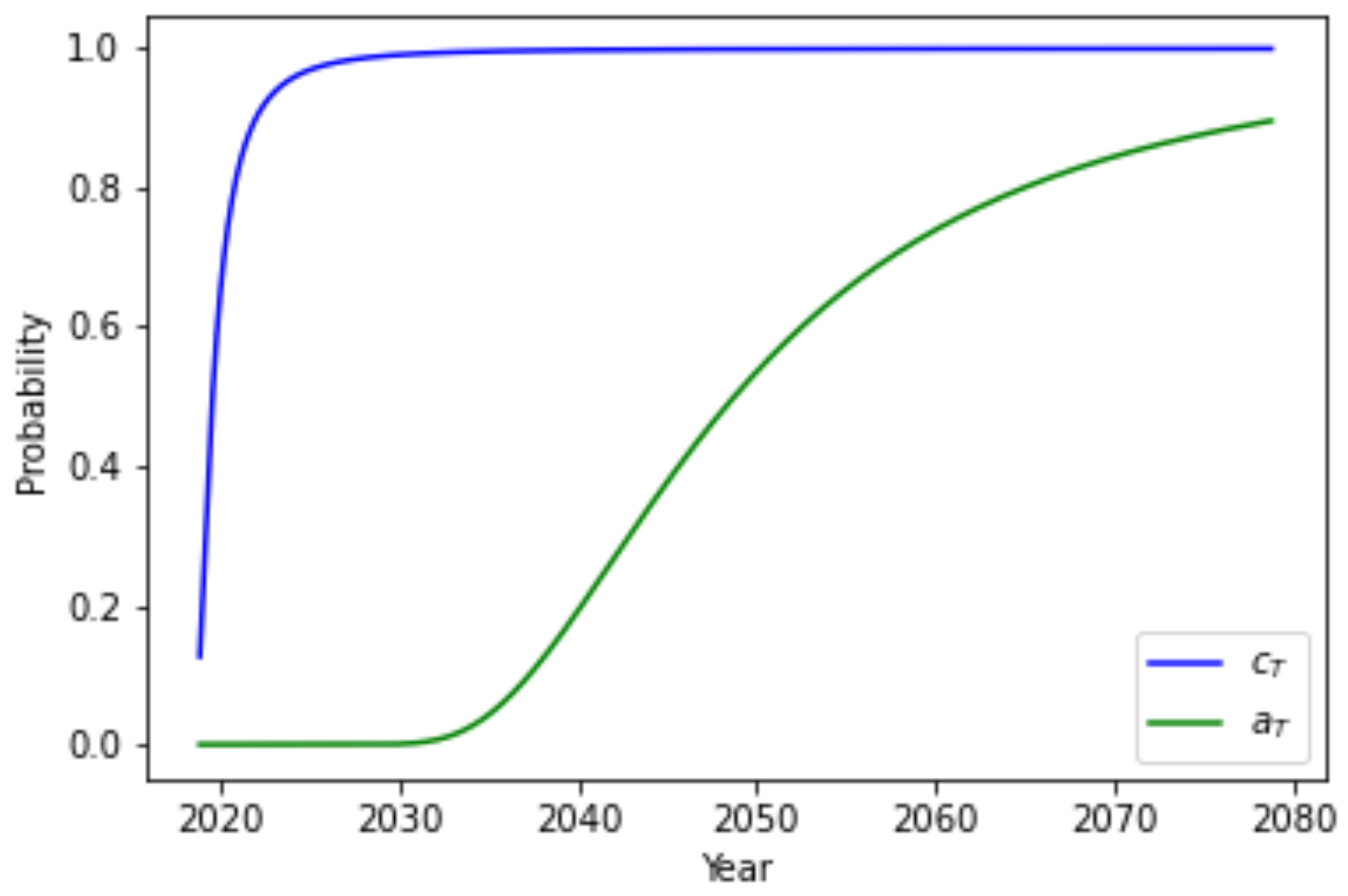
Q qubits. The development of these parameters are shown in
Figure 5.
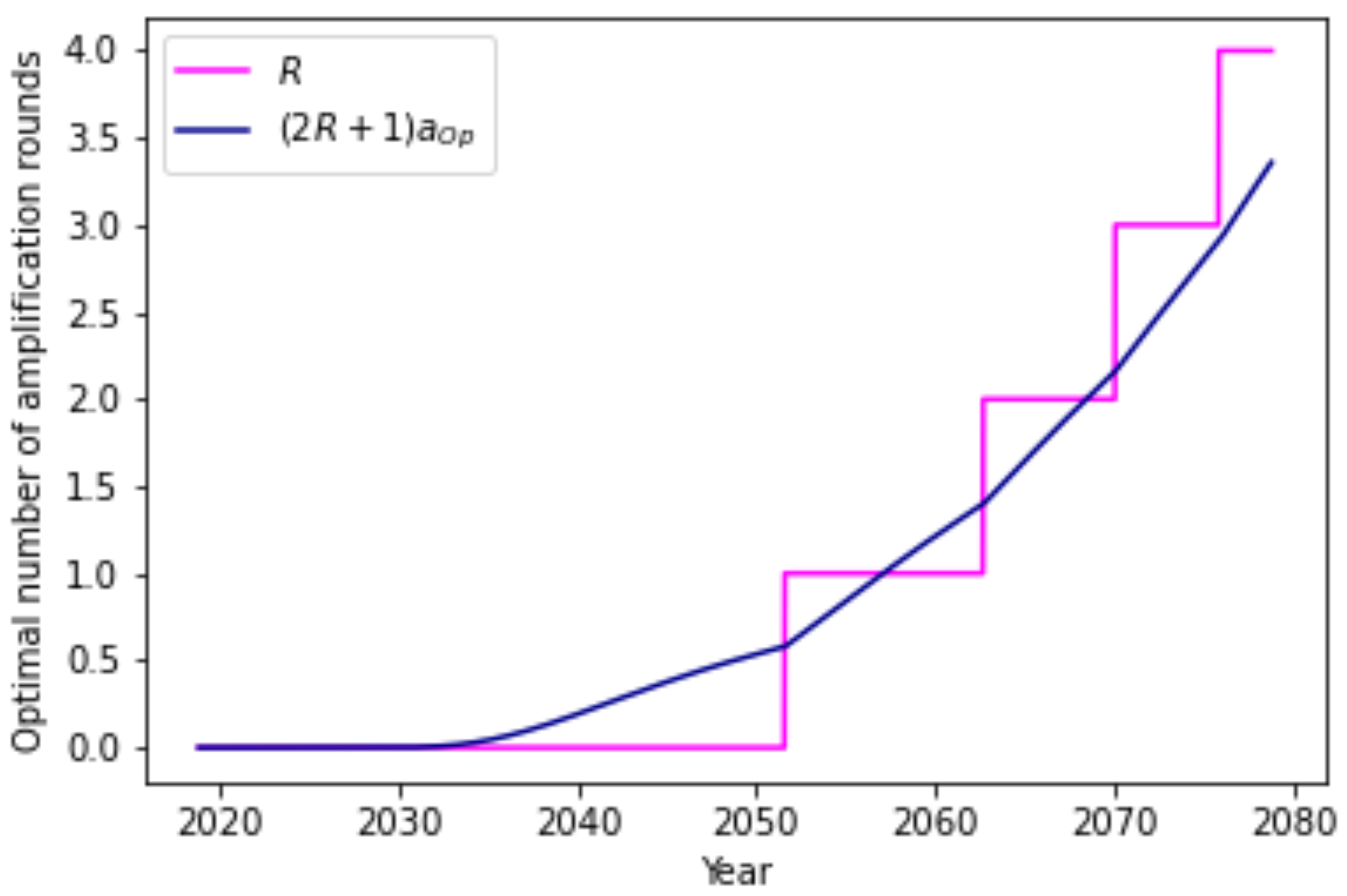
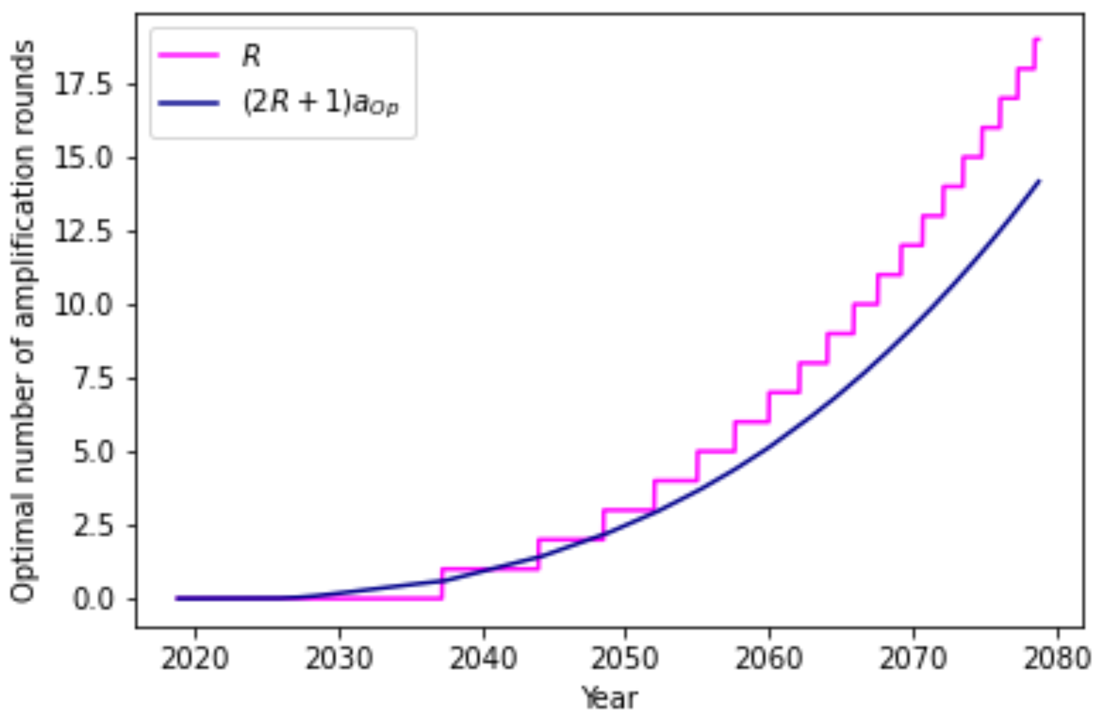
What remains to be determined is the number of amplification rounds that yields the most Fisher information per unit of time. Since each function evaluation takes the same amount of time, this is the same as maximizing the Fisher information per number of function evaluations. The optimal number of amplification rounds (
17) then is
With the increasing reliability of QV circuits, the optimal number of amplification rounds increases, as is shown in
Figure 6.
This leads to an optimal operational success probability of (
26) with the optimal number of amplification rounds. This probability decreases after the number of amplifications rounds has just increased, but this is compensated by the extra information gained from the experiments.
The common metric for the speed of a quantum computer is the circuit layer operations per second [
30] or CLOPS. This gives the number of circuit layers of a quantum volume circuit a machine can process per second. This metric is not directly applicable to other circuits. To estimate the Fisher information per second QAE may deliver in the next years, the size in gates of the transpiled and decomposed QV circuits is measured. This shows the
clops correspond to approximately
gates per second with a standard deviation of
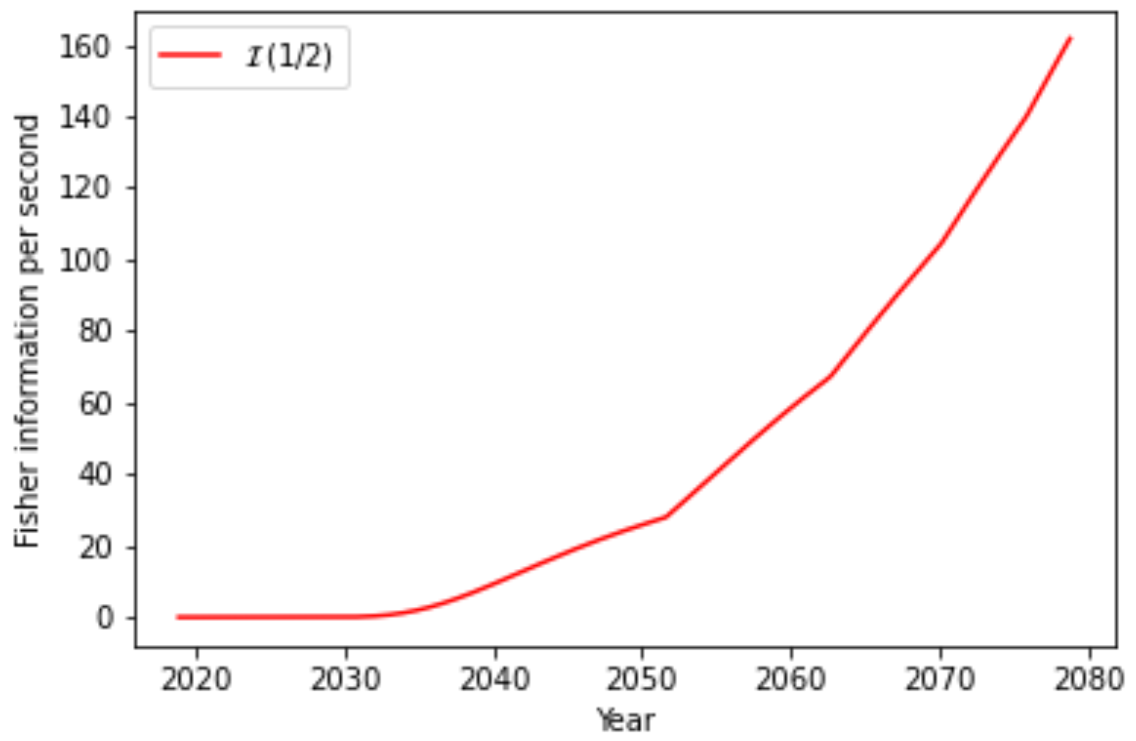
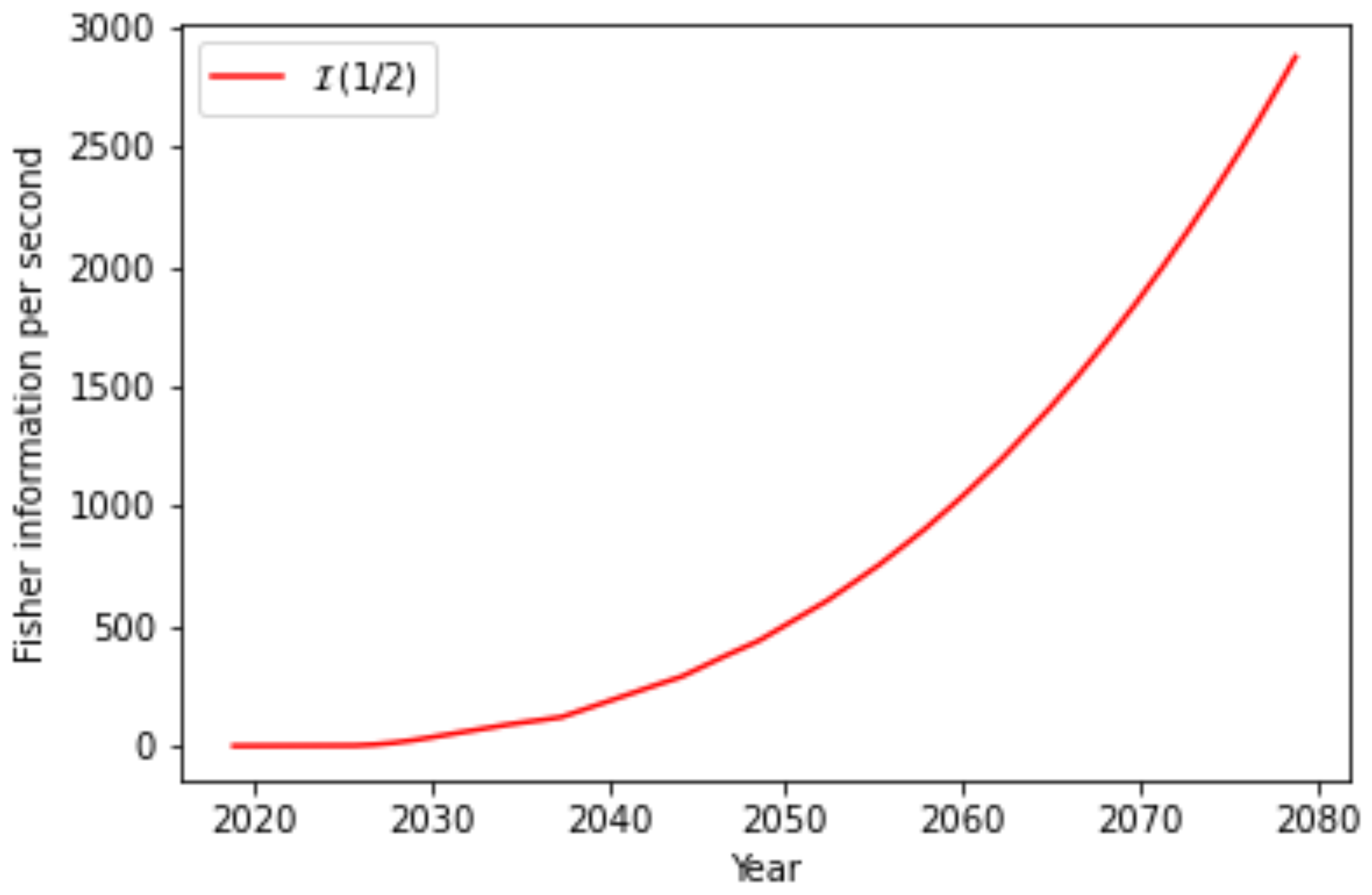
. Assuming that this number remains constant for the near future, the achievable Fisher information per second (
16) is given by
Figure 7 makes it clear that this approach for QAE will not be competitive in the coming years.
4.2. Shallow functions
The exponential increase of the size of the circuits with increasing QPU size, see (
19), demonstrates that significant changes are needed to make QAE faster than classical methods. Switching to shallow functions is an obvious option. To approximate the
samples per second a computing cluster may evaluate, this is done for QAE on
qubits, corresponding to
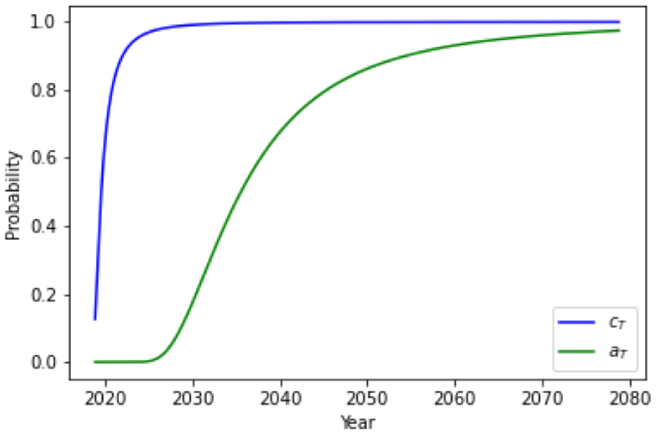
samples. Now, the analysis of the previous section can be repeated with a shallow implementation size
The results are summarized in
Figure 8,
Figure 9 and
Figure 10. This shows that the amount of Fisher information generated per second will remain much lower than classical alternatives.
5. Discussion
The methods to link the error parameters for a QAE run to that of a QV run contain various approximations and simplifications. Nonetheless, these do not trouble the bigger picture of problematically large function implementations for QAE in the near future.
An example of this is the assumption that a random state will be measured in an erroneous run of a quantum volume circuit. This is a bolder assumption than the one for QAE circuits, since the number of measured qubits is larger.
Another example is the estimated execution speed. Currently this seems lower for larger machines, but this is likely to increase in the future.
The methods used in this study are based on IBM’s quantum computing framework. These work currently with lower quantum volumes than some other constructions, but a higher speed (CLOPS). To avoid modelling the underlying reliability, connectivity and speed of the various constructions, this study has been limited to one provider.
For the relevance of the predictions on the longer term the development of better connected topologies will be of large significance. This would increase the available quantum volume and lower the implementation size of the circuits. However, the physics involved in this development places this topic out of scope here.
The variation observed in
Figure 2 suggest an imperfection in the noise model. It may be explained in part by the varying topology and the average distance for a pair of qubits. For example, adding the 12
th qubit to the processor closes the loop, see
Figure 1e,f. This results in a lower average distance and a relatively small size of the circuit implementation. As such, this would suggest a shortcoming of the noise model.
6. Conclusions
A phenomenological noise model can be used to model the error probability in a single run of a quantum volume experiment. This same model can be used in the context of quantum amplitude estimation. In this way the development of the available quantum volume of a quantum processor can be projected directly on the integration power of quantum amplitude estimation and possible many other quantum algorithms.
In this way the development of quantum amplitude estimation in the upcoming years can be estimated. The main parameter of the noise model is the size of the circuit decomposed into basis gates and transpiled for the topology of the quantum processor. This shows that both for general functions and for shallow functions the implementation size will be prohibitive to achieve an actual quantum advantages. This shows that significant improvements in the QPU are needed to achieve a quantum advantage for quantum amplitude estimation in the NISQ era.
Author Contributions
Conceptualization, methodology, formal analysis, investigation, writing—review and editing, supervision, project administration : J. de Jong ; Software, investigation, validation, resources, data curation, writing—original draft preparation, writing—review and editing, visualization: C.R. Hoek. All authors have read and agreed to the published version of the manuscript.
Funding
This work was supported by the Dutch National Growth Fund (NGF), as part of the Quantum Delta NL programme.
Data Availability Statement
Acknowledgments
We would like to thank Niels Neumann, Esteban Aguilera and Ward van der Schoot for their contributions to this project.
Conflicts of Interest
The authors declare no conflict of interest.
Abbreviations
The following abbreviations are used in this manuscript:
| CLOPS |
Circuit layer operations per second |
| MCI |
Monte Carlo integration |
| NISQ |
Noisy intermediate-scale quantum computer/era |
| QAE |
Quantum amplitude estimation |
| QPU |
Quantum processing unit |
| QV |
Quantum volume |
References
- Zaidi, H.; Andreo, P. Monte Carlo techniques in nuclear medicine dosimetry. In Monte Carlo Calculations in Nuclear Medicine (Second Edition); 2053-2563, IOP Publishing, 2022; pp. 1–1 to 1–41. [CrossRef]
- Rebentrost, P.; Gupt, B.; Bromley, T.R. Quantum computational finance: Monte Carlo pricing of financial derivatives. Physical Review A 2018, 98. [Google Scholar] [CrossRef]
- Udvarnoki, Z.; Fáth, G.; Fogarasi, N. Quantum advantage of Monte Carlo option pricing. Journal of Physics Communications 2023, 7. [Google Scholar] [CrossRef]
- Stamatopoulos, N.; Egger, D.J.; Sun, Y.; Zoufal, C.; Iten, R.; Shen, N.; Woerner, S. Option Pricing using Quantum Computers. Quantum 2020, 4, 291. [Google Scholar] [CrossRef]
- Suzuki, Y.; Uno, S.; Raymond, R.; Tanaka, T.; Onodera, T.; Yamamoto, N. Amplitude estimation without phase estimation. Quantum Information Processing 2020, 19. [Google Scholar] [CrossRef]
- Woerner, S.; Egger, D.J. Quantum risk analysis. npj Quantum Information 2019, 5. [Google Scholar] [CrossRef]
- Herbert, S. Quantum Monte Carlo Integration: The Full Advantage in Minimal Circuit Depth 2021. [CrossRef]
- Robert, C.P.; Casella, G. Monte Carlo Integration. In Monte Carlo Statistical Methods; Springer New York: New York, NY, 1999; pp. 71–138. [CrossRef]
- He, Z.; Wang, X. On the Convergence Rate of Randomized Quasi–Monte Carlo for Discontinuous Functions. SIAM Journal on Numerical Analysis 2015, 53, 2488–2503. [Google Scholar] [CrossRef]
- He, Z.; Wang, X. Convergence analysis of quasi-Monte Carlo sampling for quantile and expected shortfall. Math. Comput. 2017, 90, 303–319. [Google Scholar] [CrossRef]
- de Lejarza, J.J.M.; Grossi, M.; Cieri, L.; Rodrigo, G. Quantum Fourier Iterative Amplitude Estimation 2023.
- Tanaka, T.; Uno, S.; Onodera, T.; Yamamoto, N.; Suzuki, Y. Noisy quantum amplitude estimation without noise estimation. Phys. Rev. A 2022, 105, 012411. [Google Scholar] [CrossRef]
- Tanaka, T.; Suzuki, Y.; Uno, S.; Raymond, R.; Onodera, T.; Yamamoto, N. Amplitude estimation via maximum likelihood on noisy quantum computer. Quantum Information Processing 2021, 20. [Google Scholar] [CrossRef]
- Akhalwaya, I.Y.; Connolly, A.; Guichard, R.; Herbert, S.; Kargi, C.; Krajenbrink, A.; Lubasch, M.; Keever, C.M.; Sorci, J.; Spranger, M.; Williams, I. A Modular Engine for Quantum Monte Carlo Integration, 2023, [arXiv:quant-ph/2308.06081].
- Preskill, J. Quantum computing in the NISQ era and beyond. Quantum 2018, 2. [Google Scholar] [CrossRef]
- D’Ariano, G.M.; Macchiavello, C.; Sacchi, M.F. On the general problem of quantum phase estimation. Physics Letters A 1998, 248, 103–108, [arXiv:quant-ph/quant-ph/9812034]. [Google Scholar] [CrossRef]
- Callison, A.; Browne, D. Improved maximum-likelihood quantum amplitude estimation 2022. [CrossRef]
- Grinko, D.; Gacon, J.; Zoufal, C.; Woerner, S. Iterative quantum amplitude estimation. npj Quantum Information 2021, 7, 52. [Google Scholar] [CrossRef]
- Manzano, A.; Musso, D.; Leitao, A. Real Quantum Amplitude Estimation 2022. [2204.13641].
- Rall, P.; Fuller, B. Amplitude Estimation from Quantum Signal Processing, 2022. [CrossRef]
- Pelofske, E.; Bärtschi, A.; Eidenbenz, S. Quantum Volume in Practice: What Users Can Expect From NISQ Devices. IEEE Transactions on Quantum Engineering 2022, 3, 1–19. [Google Scholar] [CrossRef]
- Cross, A.W.; Bishop, L.S.; Sheldon, S.; Nation, P.D.; Gambetta, J.M. Validating quantum computers using randomized model circuits. Phys. Rev. A 2019, 100, 032328. [Google Scholar] [CrossRef]
- https://twitter.com/jaygambetta/status/1529489786242744320.
- https://research.ibm.com/blog/quantum-volume-256.
- https://metriq.info/.
- Ezratty, O. Understanding Quantum Technologies 2022, 2022, [arXiv:quant-ph/2111.15352].
- 2019. https://www.statista.com/chart/17896/quantum-computing-developments/.
- Brown, E.G.; Goktas, O.; Tham, W.K. Quantum Amplitude Estimation in the Presence of Noise. arXiv: Quantum Physics 2020.
- Aaronson, S.; Chen, L. Complexity-Theoretic Foundations of Quantum Supremacy Experiments. Proceedings of the 32nd Computational Complexity Conference; Schloss Dagstuhl–Leibniz-Zentrum fuer Informatik: Dagstuhl, DEU, 2017; CCC ’17.
- Wack, A.; Paik, H.; Javadi-Abhari, A.; Jurcevic, P.; Faro, I.; Gambetta, J.; Johnson, B. Quality, Speed, and Scale: three key attributes to measure the performance of near-term quantum computers. arXiv preprint arXiv:2110.14108.
| 1 |
There is no scientific reason for this odd number. |
|
Disclaimer/Publisher’s Note: The statements, opinions and data contained in all publications are solely those of the individual author(s) and contributor(s) and not of MDPI and/or the editor(s). MDPI and/or the editor(s) disclaim responsibility for any injury to people or property resulting from any ideas, methods, instructions or products referred to in the content. |
© 2023 by the authors. Licensee MDPI, Basel, Switzerland. This article is an open access article distributed under the terms and conditions of the Creative Commons Attribution (CC BY) license (http://creativecommons.org/licenses/by/4.0/).
