1. Introduction
Taiwan is located between 22°N and 25°N latitude, making it close to the equator and thus having a smaller solar angle deviation. Its advantageous geographical location provides stable sunshine, making Taiwan highly suitable for solar power development. However, Taiwan relies heavily on imported fossil fuels such as oil, coal, and natural gas, accounting for up to 92% of its energy sources, while renewable energy currently only contributes 5.5% of the total electricity generation. Within this renewable energy mix, as of 2021, solar photovoltaic power accounts for 64.8%, wind power 10.7%, and other sources such as hydroelectric and geothermal power make up 24.5% (Taipower, 2021). Therefore, more efficient development of solar energy generation has the potential to increase energy efficiency and enhance power supply reliability.
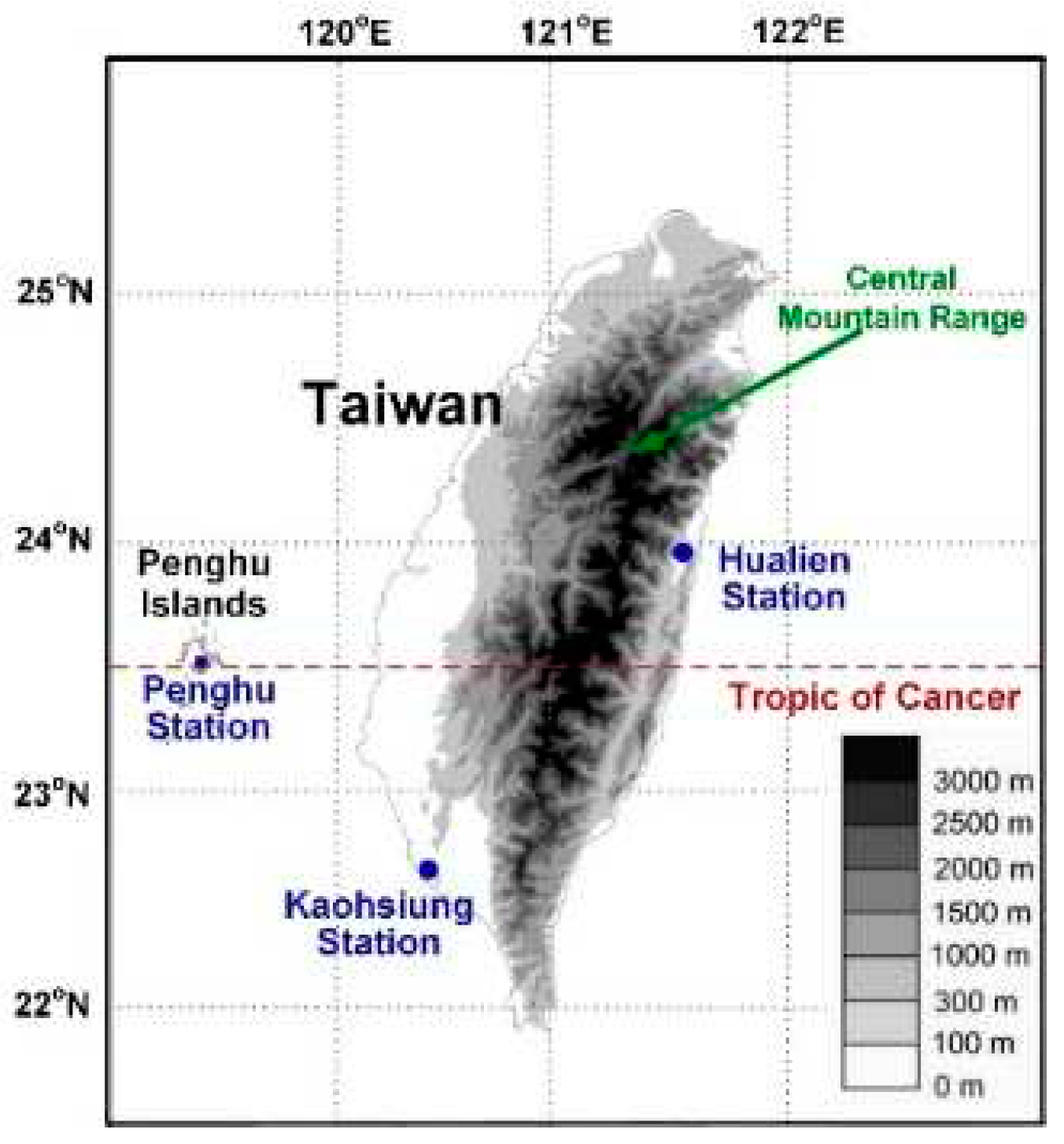
In Taiwan, the development of solar energy generation needs to take into account factors such as the angle and timing of sunlight, cloud cover, and topographical features. As a result, the energy received from solar radiation varies slightly across different regions. For example, in the southern part of Taiwan, at Kaohsiung Station (120.32°E, 22.57°N), in the eastern region at Hualien Station (121.61°E, 23.98°N), and on the outlying Penghu Islands at Penghu Station (119.56°E, 23.57°N) – as shown in
Figure 1.
Geographically, Kaohsiung Station is located south of the Tropic of Cancer, Hualien Station is situated north of the Tropic of Cancer, and Penghu Station is approximately located on the Tropic of Cancer. Regarding topographical conditions, as shown in
Figure 1, the average elevation of the Central Mountain Range (CMR) in Taiwan is about 2500 meters [
1]. The CMR divides Taiwan into two regions, with Hualien Station to the right of the CMR and Kaohsiung Station to the left. According to Taipower [
2], the solar photovoltaic electricity generation at these three meteorological stations in 2020 was 3.41, 2.85, and 3.60 kWh-d, respectively. Although these three locations are geographically close, there is a significant difference in their solar energy generation capacity.
In recent years, due to the flourishing development of machine learning, the accuracy of climate prediction has significantly improved [
3,
4,
5,
6,
7,
8,
9]. Lauret et al. [
10] used a model to predict solar radiation in island environments and proposed the use of machine learning models to enhance the performance of linear regression models. They also suggested that machine learning performs better in less stable weather conditions. Wei [
11] studied various machine learning models, such as Multilayer Perceptron and Random Forest, to analyze solar energy predictions for meteorological stations in southern Taiwan. The study compared the influence of input data from satellites, ground stations, and solar angle data on predictions. Additionally, it calculated the optimal placement angle for solar panels based on hourly solar angle data to maximize solar energy generation efficiency. Voyant et al. [
12] also utilized various machine learning methods to predict solar radiation for the next 1-6 hours. The study compared methods such as random forest, Gaussian processes, persistence, artificial neural networks, and support vector regressions to assess their strengths and weaknesses. The authors suggested that there is no one-size-fits-all best model, and combining multiple models in a hybrid prediction system yields superior results. Wei [
13] conducted research on the application of deep neural networks for predicting solar radiation. The study compared the results of backpropagation neural networks and linear regression. It also examined the impact of different types of solar panels on electricity generation efficiency. Ali et al. [
14] optimized the design of the artificial neural networks for accurate global solar radiation forecasting while minimizing computational requirements. Chodakowska et al. [
15] indicated the usefulness of ARIMA models for forecasting insolation in different geographical locations characterized by different climatic conditions.
In recent years, the recurrent neural network (RNN) architecture, which has been thriving, finds widespread applications in various fields [
16,
17,
18,
19,
20,
21,
22,
23]. Qing & Niu [
24] proposed the use of Long Short-Term Memory neural networks (LSTM) to predict solar radiation and compared the results with linear regression and backpropagation neural networks. Ultimately, they reported a 42.9% reduction in Root Mean Square Error (RMSE) for the LSTM networks compared to backpropagation neural networks in predicting solar radiation. Li et al. [
25] utilized a prediction model based on RNNs to forecast the short-term output power of a generating system. This model took only electrical data as input, without weather information, and they compared its performance within a 90-minute horizon against BPNN, Persistence, SVM, LSTM, and other methods. In recent times, many scholars have proposed the application of LSTM neural networks to predict weather changes. It is noted in the literature that most of these studies have achieved favorable forecasting results. Therefore, in this study, to enhance the accuracy of predicting long-term outcomes, the decision was made to incorporate the LSTM neural network model.
Ghofrani et al. [
26] used a clustering approach to improve the performance of Bayesian neural networks and introduced an innovative game theoretic self-organizing map (SOM) clustering method. They incorporated game theory to enhance the clustering effectiveness of the basic SOM clustering method. They also compared the results of Windows NT clustering, k-means clustering, and SOM clustering with machine learning-derived predictions. Azimi et al. [
27] proposed a k-means cluster-based algorithm to enhance the predictive performance of multilayer perceptrons. Their approach altered the initialization method of the k-means clustering algorithm to ensure consistent results each time it is trained, referred to as TB k-means. They assessed the performance of different data analysis clustering algorithms and compared the processing time required for training with different feature data. Ultimately, they suggested that this clustering approach provides better predictive results compared to directly using multilayer perceptrons.
The purpose of this study is to establish a solar radiation prediction model to accurately predict solar radiation levels. Given that solar radiation prediction is a time-series problem with highly nonlinear characteristics, this research employs various algorithmic techniques, including both unsupervised and supervised algorithms, to effectively construct suitable localized prediction models. In supervised-based algorithms, this study utilizes deep neural networks (DNN) and LSTM neural networks. Additionally, for unsupervised-based algorithms, clustering methods such as k-means clustering and fuzzy C-means clustering are employed. After clustering, subsets of data are created for each cluster, and neural network-based prediction models are established for each group. Consequently, under the DNN model, we can establish k-means DNN (referred to as k_DNN) and fuzzy C-means DNN (fc_DNN). Similarly, under the LSTM model, we can create k-means LSTM (k_LSTM) and fuzzy C-means LSTM (fc_LSTM).
2. Study Area and Material
The study was conducted in Taiwan, with test locations at Kaohsiung Station, Hualien Station, and Penghu Station (
Figure 1). The research collected ten ground-level climate parameters related to solar radiation, including atmospheric pressure, surface temperature, dew temperature, relative humidity, water vapor, average wind speed, precipitation, rainfall duration, insolation duration, and global solar radiation. The data source for these parameters was the Central Weather Administration (CWA), and the data were recorded at an hourly frequency. The data spans from 1993 to 2021, totaling 29 years, resulting in a total of 254,184 hourly records.
Table 1 presents the attributes along with their respective units and statistical values.
According to Wei [
11], the addition of solar angle parameters can be used to improve the prediction of global solar radiation. Therefore, this study includes five solar angle parameters, namely the declination angle, hour angle, zenith angle, elevation angle, and azimuth angle [
28]. Firstly, the declination angle (
δ) is the angle between the line connecting the sun and the center of the Earth and the plane of the equator. The formula for this angle is as follows:
The hour angle (
ω) represents the angle that the sun moves relative to the position of the station per hour and can be calculated as follows:
The zenith angle (
θ) is the angle between the sun and the vertical line to the horizontal plane and can be calculated using the following formula:
The elevation angle (
α) is the angle between the line connecting the Sun to the observation point and the horizontal plane.
The azimuth angle (
ξ) is the angle between the sun's position in its orbit and the horizontal plane. It can be calculated using the following formula:
In the equations (1) to (5) mentioned above, where nd represents the day of the year, ranging from 1 to a maximum of 365; H represents the hour of the day when the angle is calculated, ranging from 1 to 24 hours; and λ denotes the latitude of the test location.
3. A Real-time Prediction System
As predicting solar radiation cannot guarantee that a single model will provide the best forecast [
12], this study establishes a real-time solar radiation prediction system. It aims to integrate simulation results from different models, following the concept of an ensemble model to jointly determine the optimal solution.
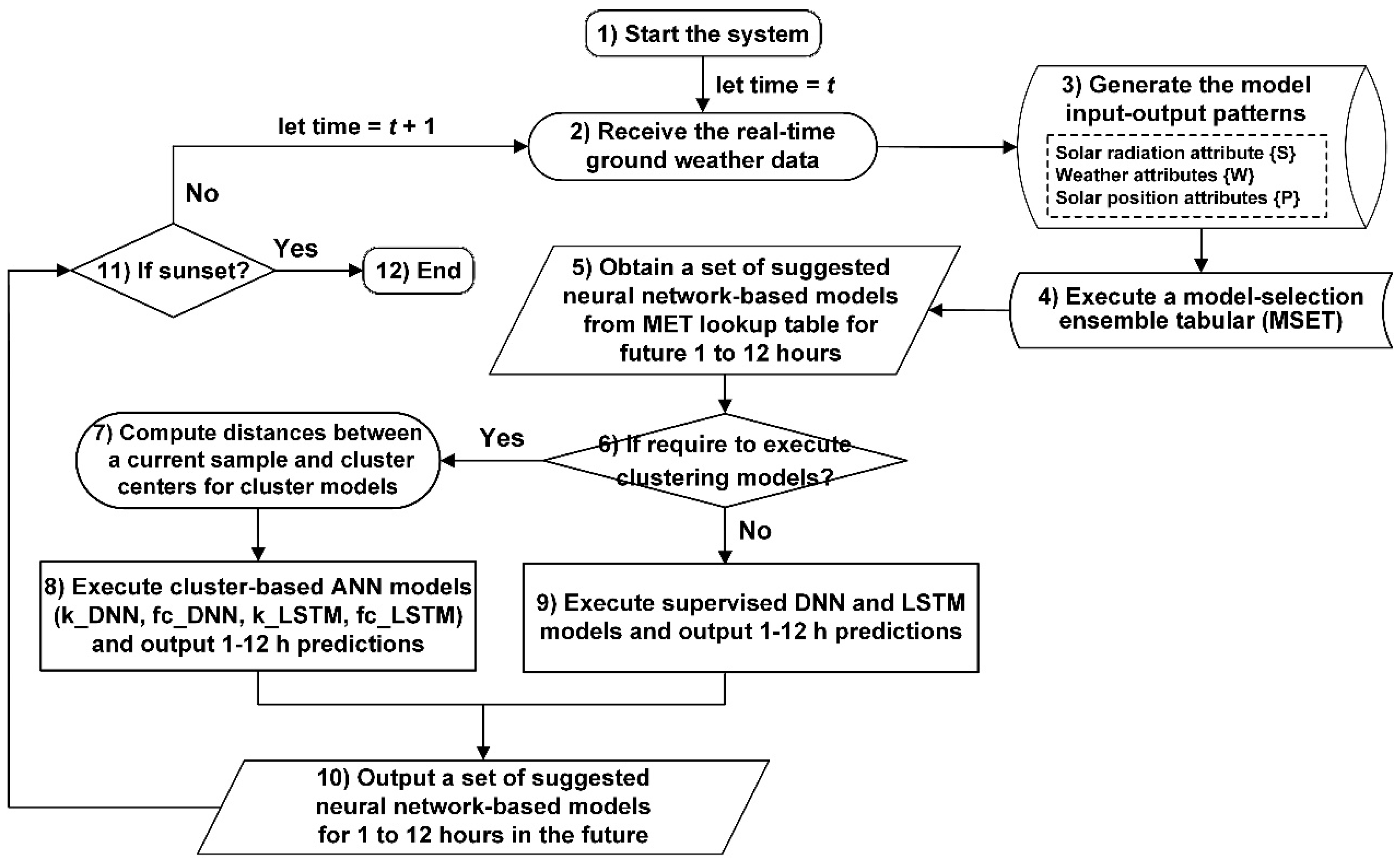
Figure 2 illustrates the real-time prediction concept process designed for this study. The simulation interval is 1 hour, and the solar radiation forecast horizon ranges from 1 to 12 hours. The steps are described as follows:
- 1)
At sunrise, set the time as t;
- 2)
Receive the real-time ground weather data;
- 3)
Generate model input patterns, including the global solar radiation attribute {S}, weather attributes {W}, and solar position attributes {P}. The dataset {P} {δ, ω, θ, α, ξ} can be derived from Equations (1)-(5);
- 4)
Execute a model selection ensemble tabular (abbreviated as MSET);
- 5)
Retrieve the set of optimal suggested neural network-based models from the MSET lookup table for the future 1 to 12 hours;
- 6)
Is it necessary to execute clustering models based on the suggested neural network-based models? If "yes," proceed to step 7; if "no," go to step 9;
- 7)
Calculate the distances between a current sample and cluster centers for cluster models;
- 8)
Execute cluster-based models (i.e., k_DNN, fc_DNN, k_LSTM, and fc_LSTM) and generate 1-12 hour predictions;
- 9)
Execute DNN and LSTM models and generate 1-12 hour predictions;
- 10)
Generate a set of suggested neural network-based models for 1 to 12 hours in the future;
- 11)
Is it sunset? If "yes," conclude the analysis procedure (Step 12); if "no," return to step 2 and set the time as t + 1.
In step 4, the lookup table from MSET is used to determine the optimal model for real-time predictions at each forecasting time (1 to 12 hours). Compared to having a single model decide the forecast, the collaborative decision of all models can enhance accuracy. In steps 8 and 9, the methods for establishing each model will be explained as follows.
3.1. Supervised models
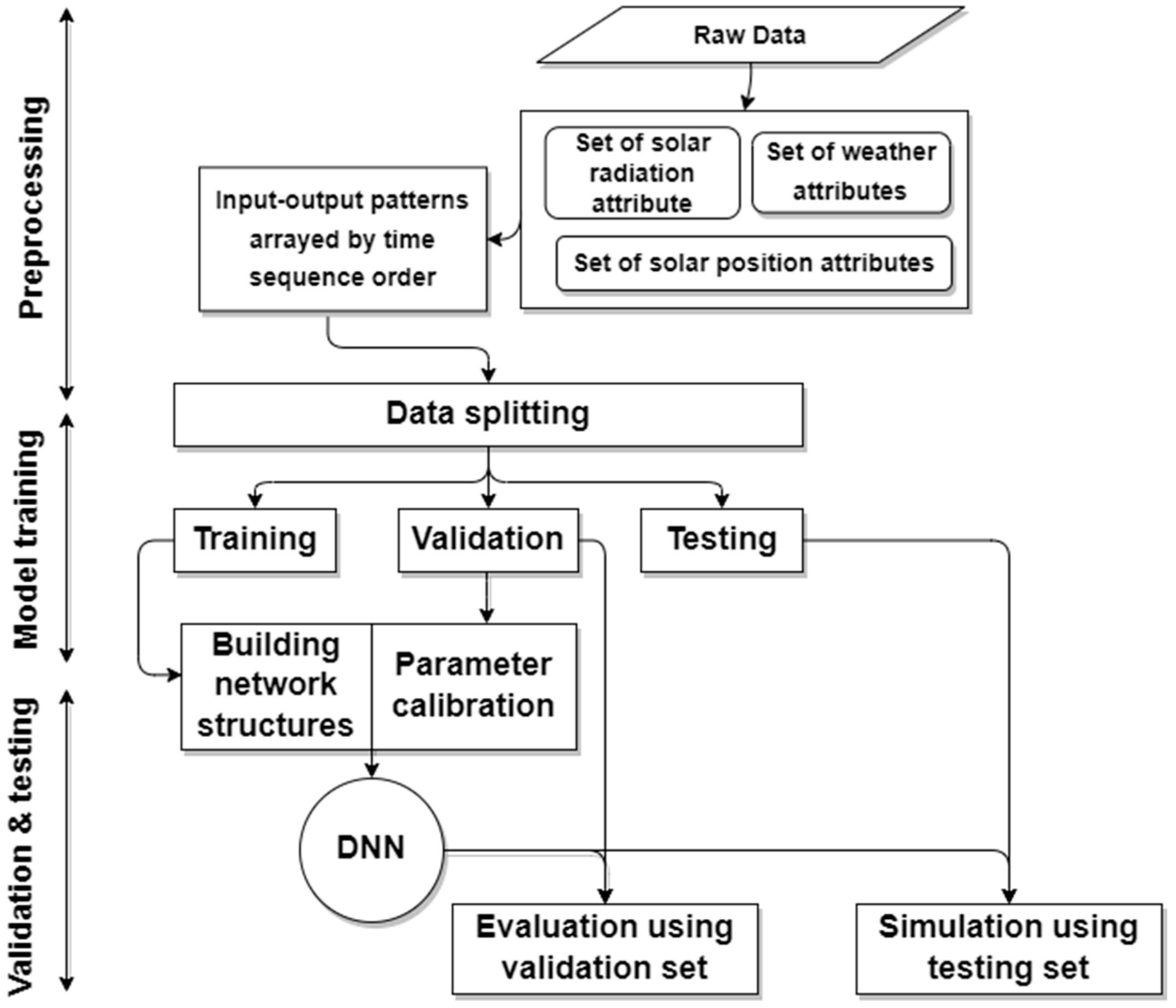
Figure 3 illustrates the modeling process for supervised models. Taking DNN as an example, DNN is developed based on the structure of deep neural networks. A deep neural network is a model with multiple layers, an advanced development of the multilayer perceptron based on the principles of the multilayer perceptron. The multilayer perceptron includes an input layer, hidden layers, and an output layer. The input layer of the multilayer perceptron serves as the interface for external input information, while the hidden layers and the output layer perform the actual computations. The flowchart in
Figure 3 explains that the data sets consist of the solar radiation attribute {
S}, weather attributes {
W}, and solar position attributes {
P}. These three data sets are organized in a time sequence and then divided into a training set, a validation set, and a testing set. The training set and validation set are used for building prediction models, while the testing set is used to evaluate the model's performance.
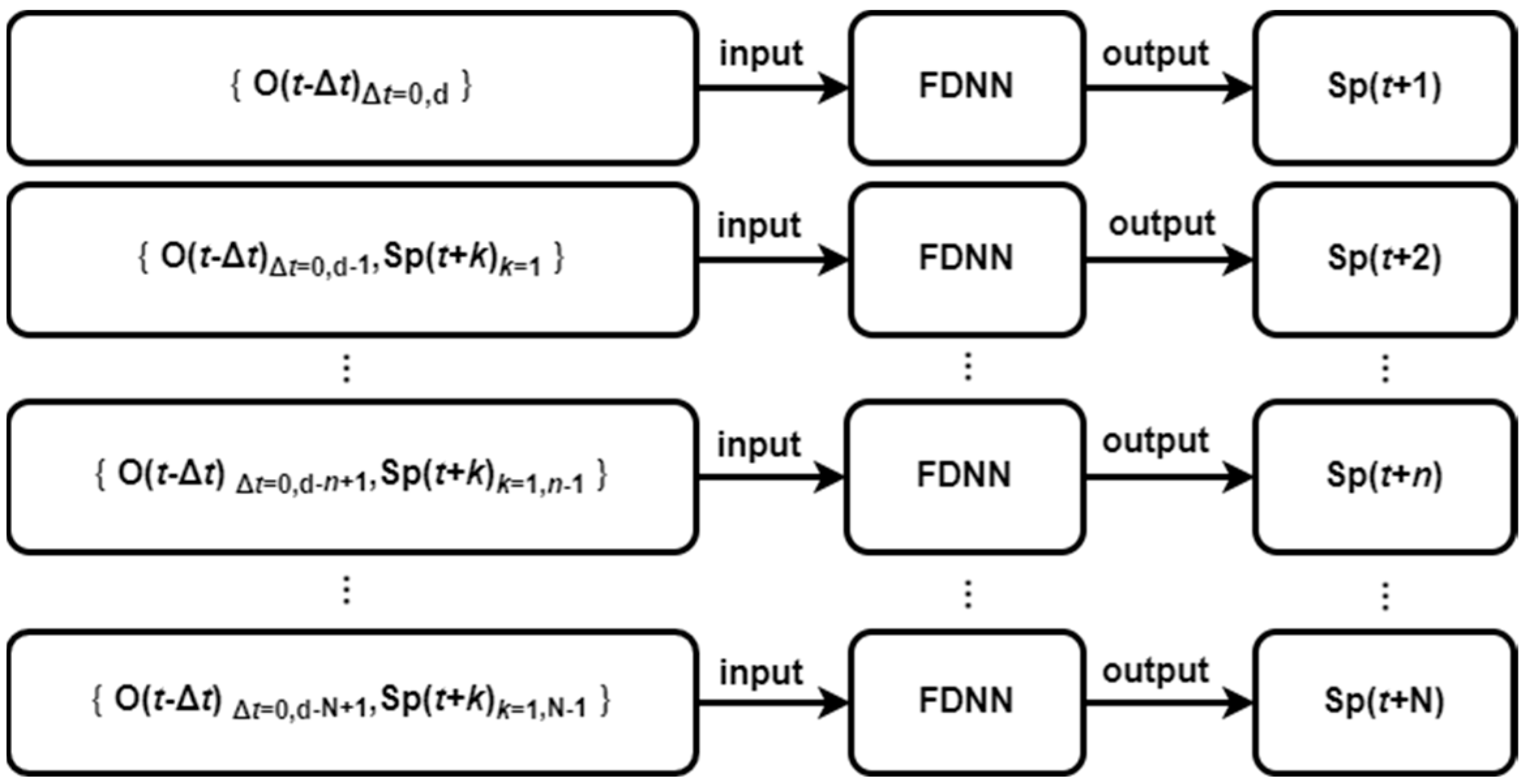
As shown in
Figure 4, O() represents a collection of observed values, including datasets of {
S}, {
W}, and {
P}. S
P() represents a collection of predicted solar radiation values. The predictive function of the model can be written as:
where S
P(
t+
k) represents the predicted solar radiation value for the future
k hours, O(
t−Δ
t) denotes past observed data,
d is the input delay time for the model,
N is the maximum prediction time length (set as a constant value in this study,
N = 12 hours), and
n and
k are parameters (indices) for the prediction time length.
In Eq. (6), when predicting the solar radiation SP(t+1) for the next 1 hour, the current time data (Δt = 0) and the observation set of the past d hours are used. For predictions beyond t+2 in the future, the previous predicted values for each time step are also incorporated.
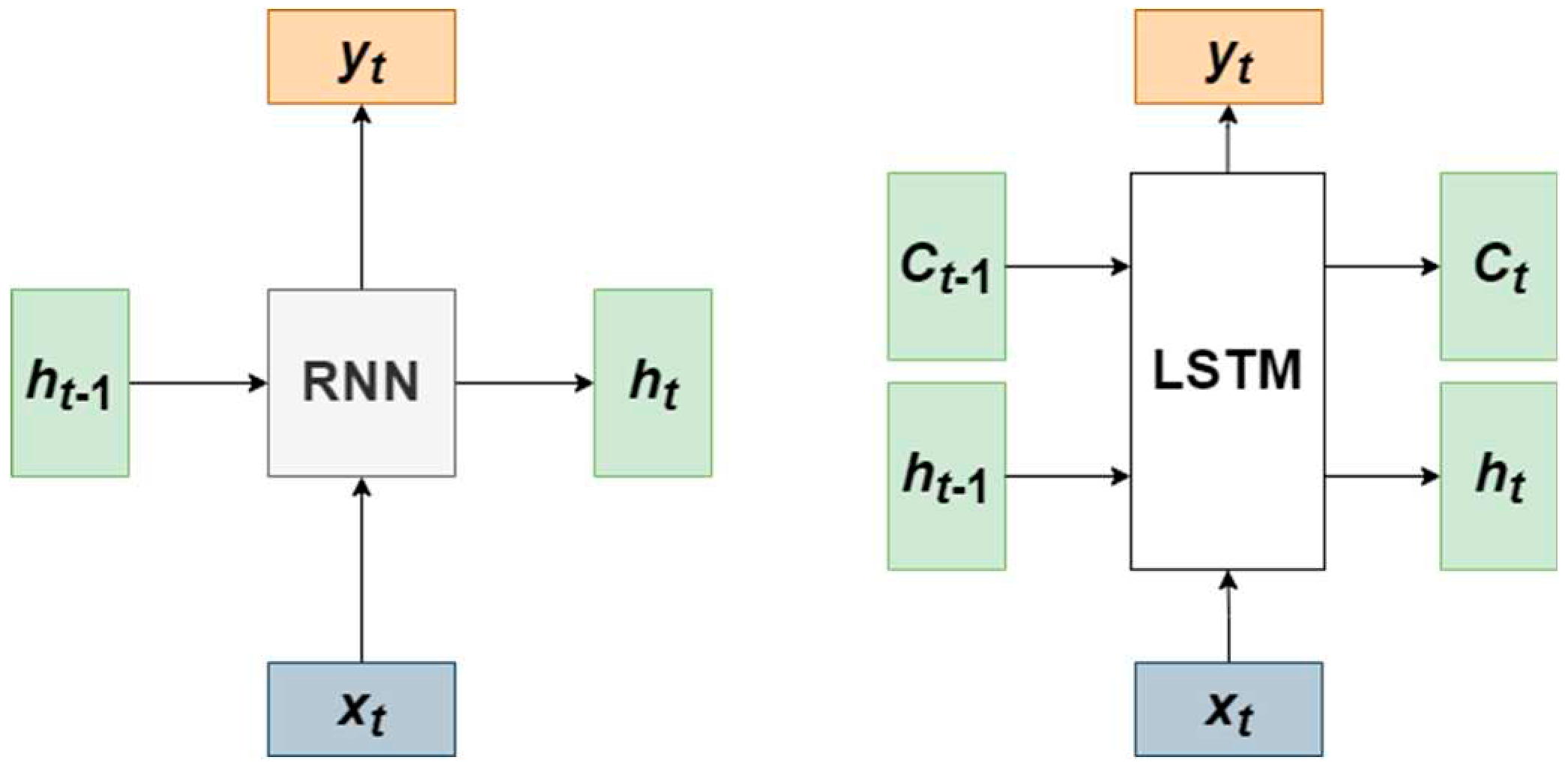
Additionally, in this study, another supervised model is employed, namely LSTM. LSTM is an advanced model within RNN. RNNs are recurrent networks commonly used for handling time and sequence-related problems. However, during the modeling process, the issue of vanishing gradients or exploding gradients may occur. To address this problem, Hochreiter & Schmidhuber [
29] introduced the LSTM neural network, which is an improved model incorporating memory blocks within the hidden layers of the RNN. As shown in
Figure 5, while traditional RNNs have a single hidden state
ht, LSTM networks introduce memory blocks
Ct, allowing them to retain longer memories and forget less relevant information.
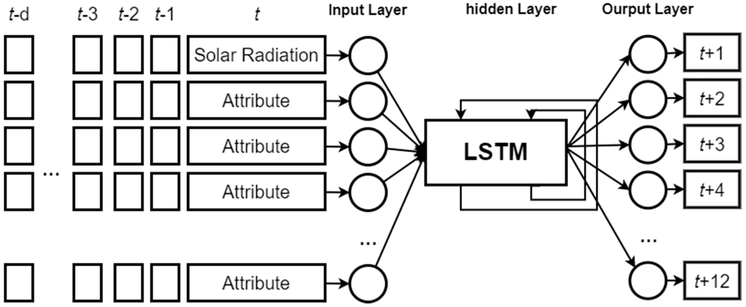
In the construction of the LSTM model in this study, the input data comprises the current solar radiation {
S} and attributes {
W} and {
P}. The input-output format of the model, as shown in
Figure 6, involves sequentially feeding data into the model based on the time sequence. The LSTM model is trained to predict 12 target values (i.e., solar radiation for the next 12 hours), with each input data entry having a time length of
d'. The model directly outputs predictions for the next 12 hours. To assess accuracy, the data is split into three sets for training, validation, and testing, as illustrated in
Figure 3, to evaluate the model's performance.
3.2. Unsupervised combined supervised models
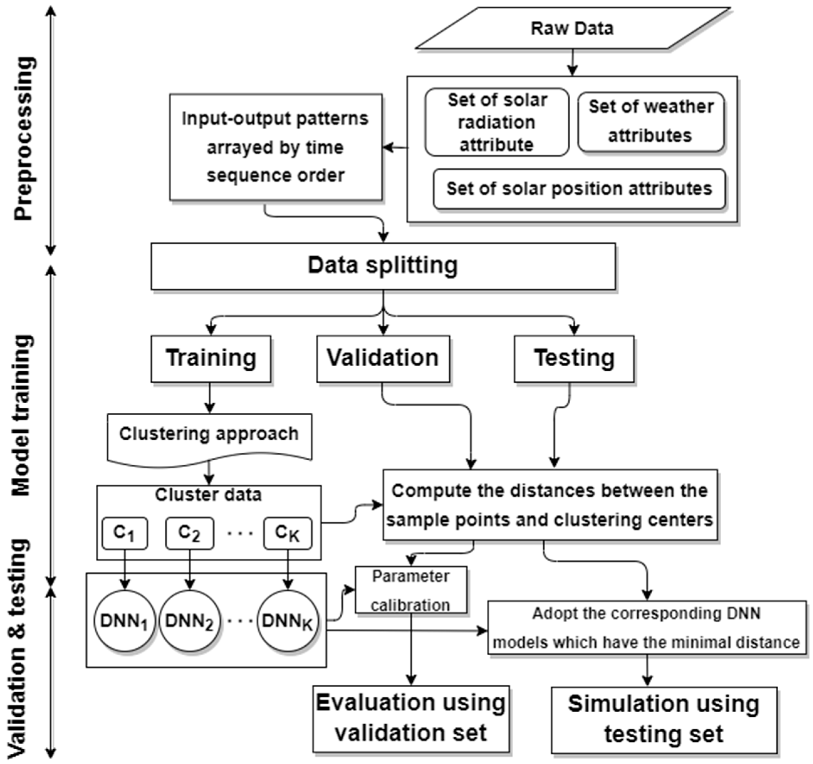
The unsupervised combined with supervised models in this study utilize unsupervised clustering algorithms in conjunction with supervised neural networks to form an integrated framework. The modularized process is depicted in
Figure 7. Initially, the three data sets of {
S}, {
W}, and {
P} are arranged based on the time sequence and then undergo data splitting. Subsequently, the training set is clustered, and each group of data is used to train a single supervised model (such as DNN and LSTM). After the model construction is complete, each data point in the validation set identifies the cluster center with the shortest distance and utilizes the corresponding ANN model for that cluster to predict solar radiation.
This study utilizes two clustering methods: k-means and fuzzy C-means. The k-means is a clustering algorithm that groups n data points into k clusters by minimizing the sum of squared distances between all data points and their respective cluster centroids. The objective function J
K is the sum of squared distances between all data points and their cluster centroids, and the mathematical expression is as follows:
where K is the number of clusters;
k is the cluster index;
n is the number of data points;
xj is the
j-th input data sample;
Ci is the centroid of the
i-th cluster;
wji is a weight, which is 1 if the data belongs to the
i-th cluster, and 0 otherwise.
The fuzzy C-means algorithm applies fuzzy theory concepts to clustering methods [
30]. Unlike k-means, in fuzzy C-means, the weights
W are not binary; instead, each attribute data is represented by a membership function to indicate the degree of belonging to each cluster. The objective function J
C is the sum of the squared distances between all data points and their cluster centroids, as shown in the following equation:
where K is the number of clusters,
n is the number of data points,
xj represents the
j-th sample data,
Ci is the centroid of the
i-th cluster,
is the weight (ranging from 0 to 1) indicating the degree of truth for its fuzzy set, and
m is the exponent coefficient, typically set to 2.
The sum of the weight coefficients should satisfy the constraint as follows:
The weight formula is as follows:
The number of clusters K mentioned above will be determined using a trial and error method.
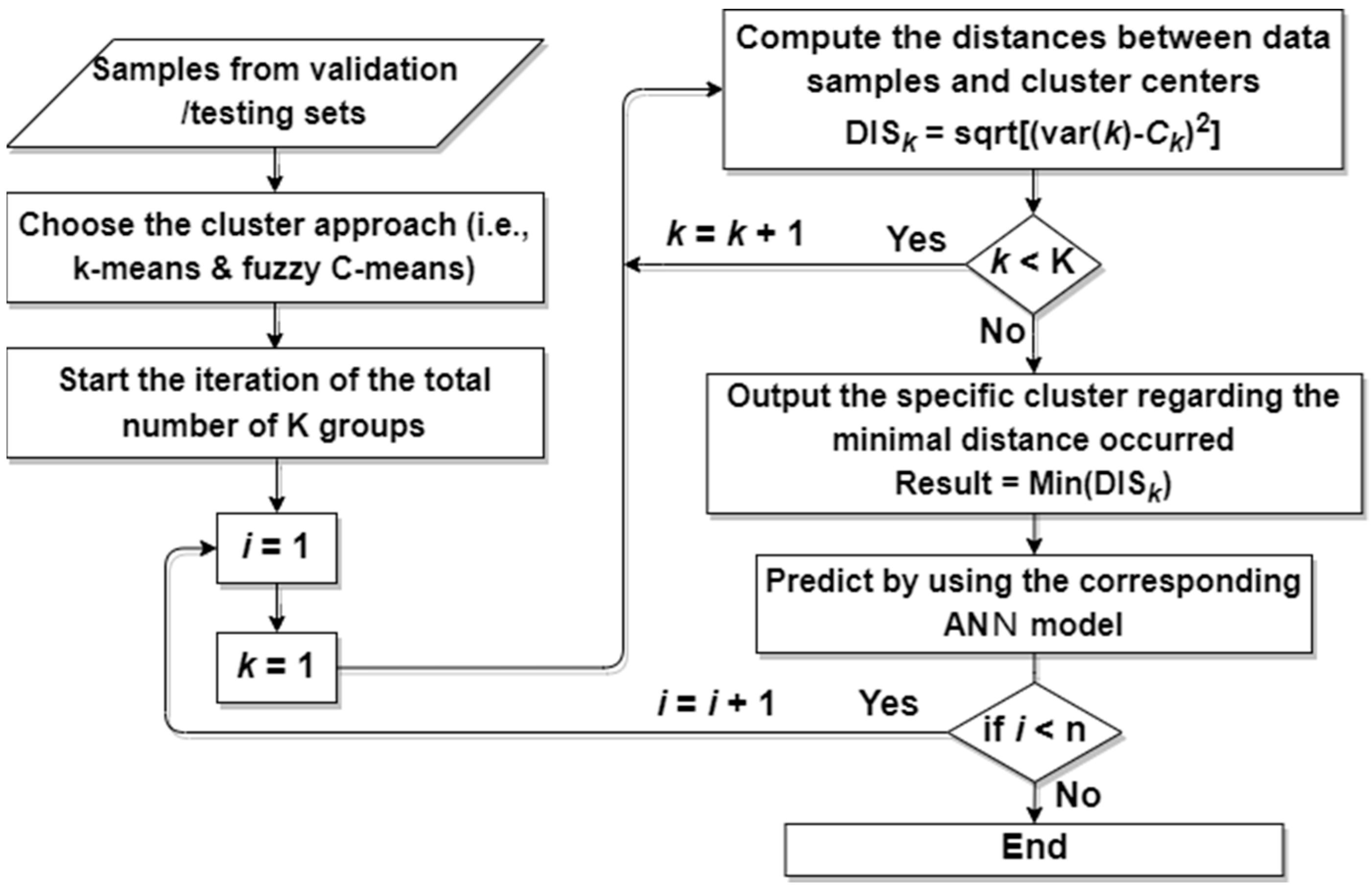
Figure 8 illustrates the process of selecting a cluster and predicting solar radiation based on the data in the validation set and testing set. After selecting the clustering method, the distance DIS between sample point
i and cluster center
Ck is calculated.
kmin_dis represents the shortest distance to a certain cluster. Based on the
kmin_dis result, you can use the predictive model associated with that cluster to estimate solar radiation.
4. Modeling and Results
This study divides the data from the experimental locations (i.e., Kaohsiung Station, Hualien Station, and Penghu Station) into training data for 18 years (1993 to 2010), validation data for 6 years (2011 to 2016), and testing data for 5 years (2017 to 2021). Python programming language and the Keras library were used to build machine learning models and perform computations. The evaluation metrics employed in this study include RMSE (root mean squared error) and rRMSE (relative RMSE), with the formulas as follows:
where
M is the number of data points;
represents the
ith prediction value;
is the
ith observed value, and
is the mean of all observed values.
4.1. Parameter calibration
The hyperparameters for the DNN model need to be tuned, including the learning rate, momentum, the number of hidden layers, and the number of neurons in a hidden layer. The learning rate controls the step size for weight updates and affects the convergence speed. A learning rate that is too small can lead to slow convergence, while a learning rate that is too large can cause oscillations. This study started with a learning rate of 0.001 and increased it gradually in steps of 0.001 to find the optimal learning rate. Momentum is an effective way to enhance the efficiency of weight adjustments. It involves incorporating part of the previous learning's value to update the network's weights, which can significantly reduce the influence of extreme values or noise in the data. This study experimented with momentum values in the range of 0.01, increasing by 0.01 in each step. The number of hidden layers in the network is another crucial hyperparameter. This study tested architectures with 1 to 3 hidden layers. The number of neurons in a hidden layer influences the network's ability to generalize. Too few neurons can lead to underfitting, while too many neurons can lead to overfitting. The study explored the number of neurons, starting from 1 and gradually increasing up to 50 to determine the optimal configuration.
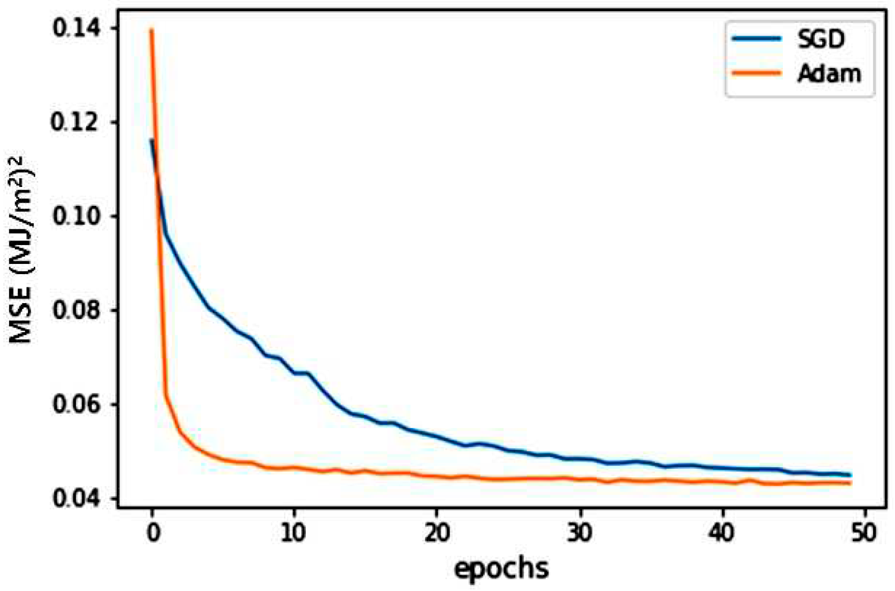
In the DNN modeling process, the performance of two optimizers, namely Stochastic Gradient Descent (SGD) and Adaptive Moment Estimation (Adam), was initially compared.
Figure 9 illustrates the iterative convergence process of errors using these two optimizers for Kaohsiung Station. It is evident that Adam outperforms SGD in terms of error convergence. As a result, Adam optimizer was chosen for subsequent steps.
Next, this study determines the delay time length,
d.
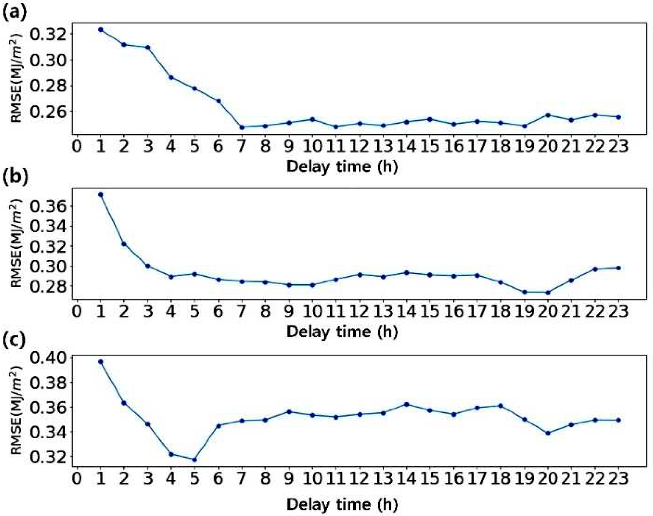
Figure 10 presents the best RMSE at various delay times under the Adam optimization. With the increase in
d, the error reduction is less pronounced. This study uses
d = 7 hours, 10 hours, and 5 hours as parameter values for Kaohsiung, Hualien, and Penghu Station, respectively.
Table 2 lists the parameter tuning results for the number of hidden layers and the number of neuron nodes in the DNN (
t+1) model under the Adam optimization for the next hour (
t + 1). Using the same method, we conducted parameter tuning for 1 to 12 hours into the future.
In the case of building the LSTM models, the parameter
d' represents the length of data required for the LSTM input. The values of
d determined in the previous section for the DNN model can serve as reference values for
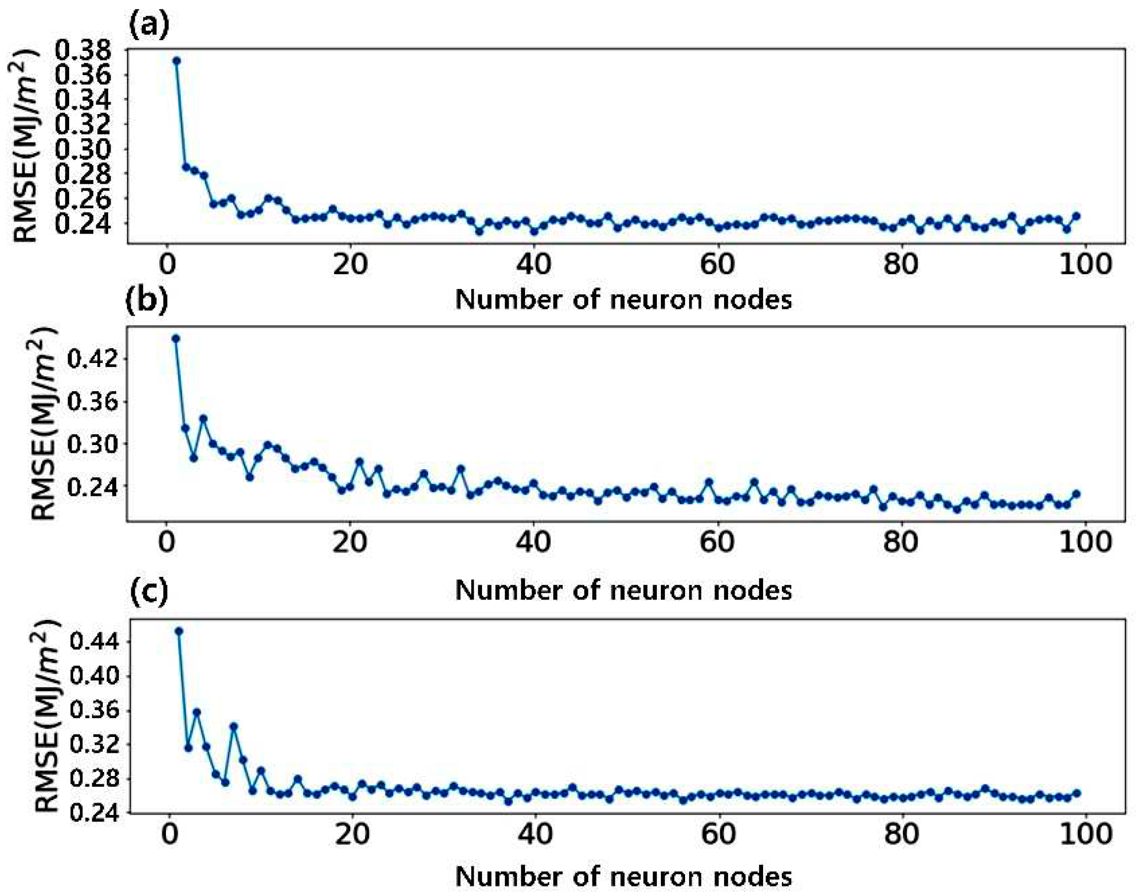
d', which are assumed to be 7, 10, and 7 hours for the three experimental stations, respectively. The number of LSTM neurons was tested for forecast horizons from 1 to 12 hours. Taking the example of the
t+1 forecast,
Figure 11 shows that Kaohsiung, Hualien, and Penghu Stations achieved stable convergence errors with 39, 85, and 36 neurons, respectively.
In the cluster-based DNN and LSTM models, during the clustering algorithm process, this study examined the number of clusters and determined the optimal number of clusters.
Figure 12 shows the trial-and-error process for determining the number of clusters for k_DNN, fc_DNN, k_LSTM, and fc_LSTM. The results reveal that for the DNN models, the optimal number of clusters for Kaohsiung Station, Hualien Station, and Penghu Station were 4, 3, and 4 for k_DNN and 5, 4, and 5 for fc_DNN. For the LSTM models, k_LSTM had an optimal number of clusters of 5, 4, and 5, and fc_LSTM had an optimal number of clusters of 5, 5, and 5. The results indicate that both DNN and LSTM models achieve their best performance with fewer than 5 clusters.
5. Simulation
This study evaluated the DNN, LSTM, k_DNN, fc_DNN, k_LSTM, and fc_LSTM models using the testing set.
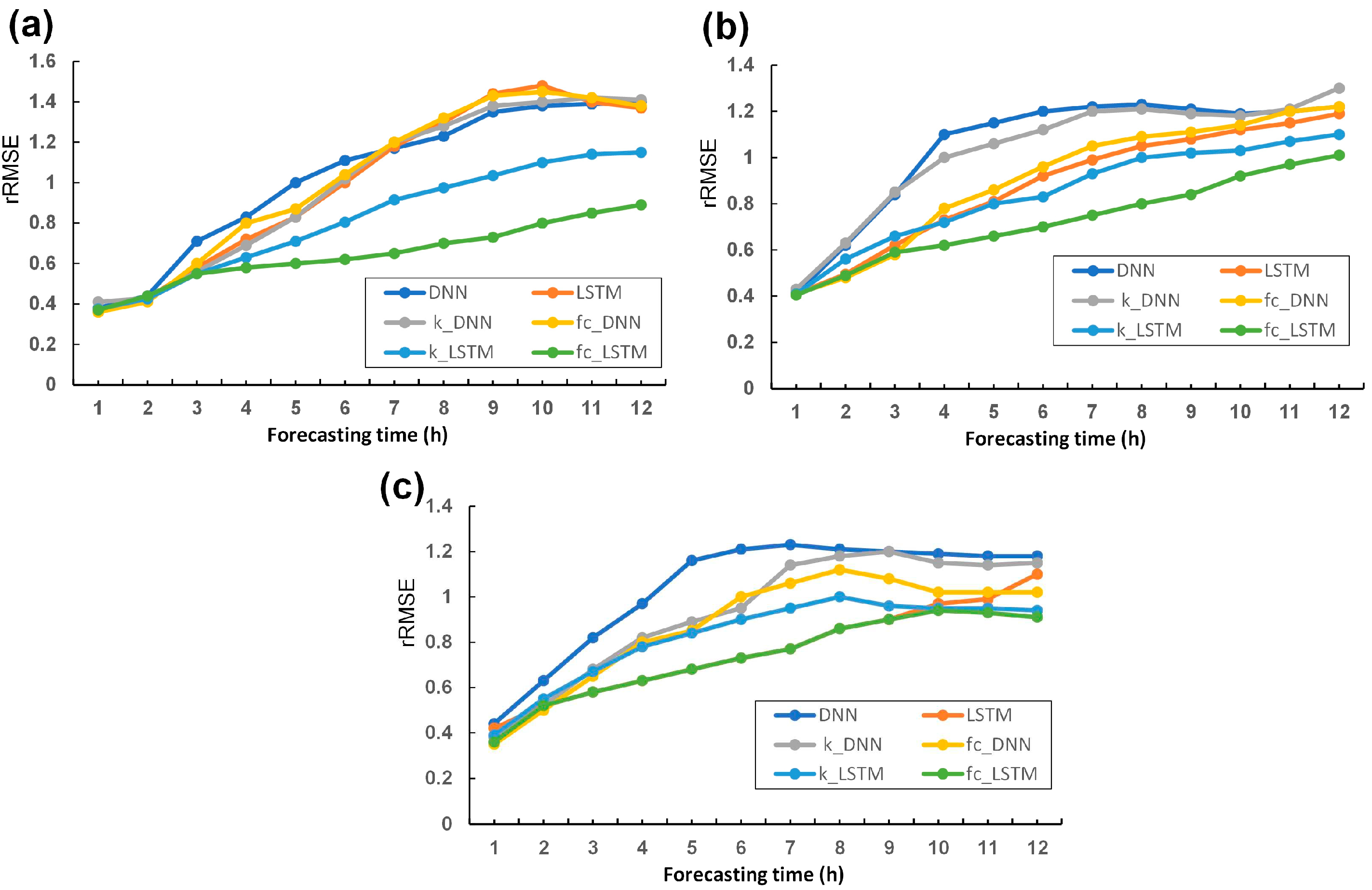
Figure 13 presents the evaluation results using the testing set, showing the rRMSE performance of each model for lead times ranging from 1 to 12 hours. From
Figure 13a, it can be observed that at Kaohsiung Station, for lead times of 1 to 2 hours, the different models have similar rRMSE values. However, for lead times greater than 3 hours, fc_LSTM exhibits superior prediction performance. In
Figure 13b, at Hualien Station, for lead times of 1 to 3 hours, LSTM, fc_DNN, and fc_LSTM show comparable rRMSE values. For lead times greater than 4 hours, fc_LSTM demonstrates better prediction performance.
Figure 13c shows the results for Penghu Station, where for lead times of 1 to 2 hours, k_DNN, LSTM, k_LSTM, fc_DNN, and fc_LSTM models have similar rRMSE values. However, for lead times greater than 3 hours, fc_LSTM exhibits a more significant advantage in terms of prediction performance.
Based on the rRMSE results of the DNN model, this study defined a "model improvement rate," as described below:
After calculation, it was found that at all three stations, the fc_LSTM model had the highest improvement rate (improving by 37.27%, 30.41%, and 29.08% respectively), followed by the k_LSTM model with the second-highest improvement rate (improving by 20.81%, 19.54%, and 29.08% respectively).
Table 3.
Average performance levels for 1–12 h predictions.
Table 3.
Average performance levels for 1–12 h predictions.
| Station |
Measure |
DNN |
LSTM |
k_DNN |
fc_DNN |
k_LSTM |
fc_LSTM |
| Kaohsiung |
RMSE (mj/m2) |
0.601 |
0.570 |
0.567 |
0.574 |
0.457 |
0.342 |
| |
rRMSE |
1.033 |
1.008 |
1.003 |
1.023 |
0.818 |
0.648 |
| |
IR |
0% |
2.42% |
2.90% |
0.97% |
20.81% |
37.27% |
| Hualien |
RMSE (mj/m2) |
0.519 |
0.454 |
0.501 |
0.497 |
0.430 |
0.364 |
| |
rRMSE |
1.049 |
0.880 |
1.032 |
0.907 |
0.844 |
0.730 |
| |
IR |
0% |
16.11% |
1.62% |
13.54% |
19.54% |
30.41% |
| Penghu |
RMSE (mj/m2) |
0.503 |
0.401 |
0.437 |
0.421 |
0.389 |
0.352 |
| |
rRMSE |
1.035 |
0.823 |
0.933 |
0.873 |
0.763 |
0.734 |
| |
IR |
0% |
20.48% |
9.86% |
15.65% |
26.28% |
29.08% |
5.1. Model selection ensemble tabular (MSET)
From
Section 3 of the real-time prediction system, the lookup table from MSET is used for real-time predictions to determine the best model for each forecast time (1 to 12 hours).
Table 4 presents the results obtained from testing data simulations. It is observed that for short-term predictions (lead time <= 3 h), a combination of clustering algorithms with DNN or LSTM models performs better at all three stations. However, for long-term predictions (lead time >= 4 h), combining clustering algorithms with LSTM models is the most stable choice.
Table 4.
Model selection ensemble tabular (MSET).
Table 4.
Model selection ensemble tabular (MSET).
| Lead time |
Kaohsiung Station |
Hualien Station |
Penghu Station |
| 1 h |
fc_DNN |
fc_DNN |
fc_DNN |
| 2 h |
fc_DNN |
fc_DNN |
fc_LSTM |
| 3 h |
fc_LSTM |
fc_DNN |
fc_LSTM |
| 4-12 h |
fc_LSTM |
fc_LSTM |
fc_LSTM |
This study uses test data from 2017 for simulating the real-time prediction system. The best models selected from the MSET table for different forecast periods are further utilized for real-time updates in predicting solar radiation. To assess the system, ground station data and solar angle data obtained through k-means and fuzzy C-means clustering are used. Each set of data belongs to a cluster with cluster center coordinates. The model selection set table can be updated based on the required time intervals to ensure the accuracy of clustering and statistical results. In practice, current data is imported into the database every hour. The best forecast models for each upcoming hour are defined according to the model selection set table, and the results of all models are computed. Finally, the required forecast values are combined, and the current time is adjusted, enabling continuous predictions until the user terminates the process.
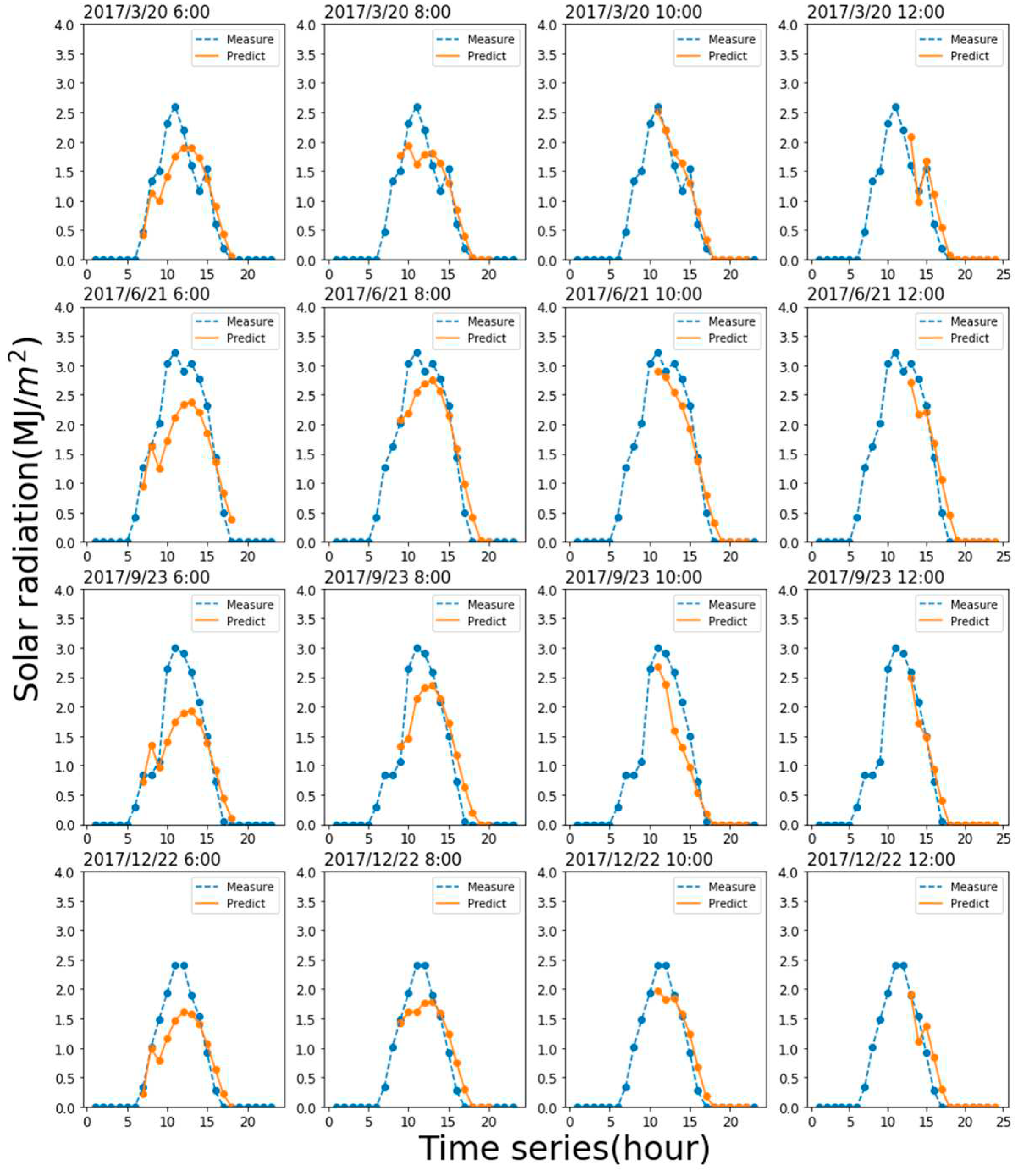
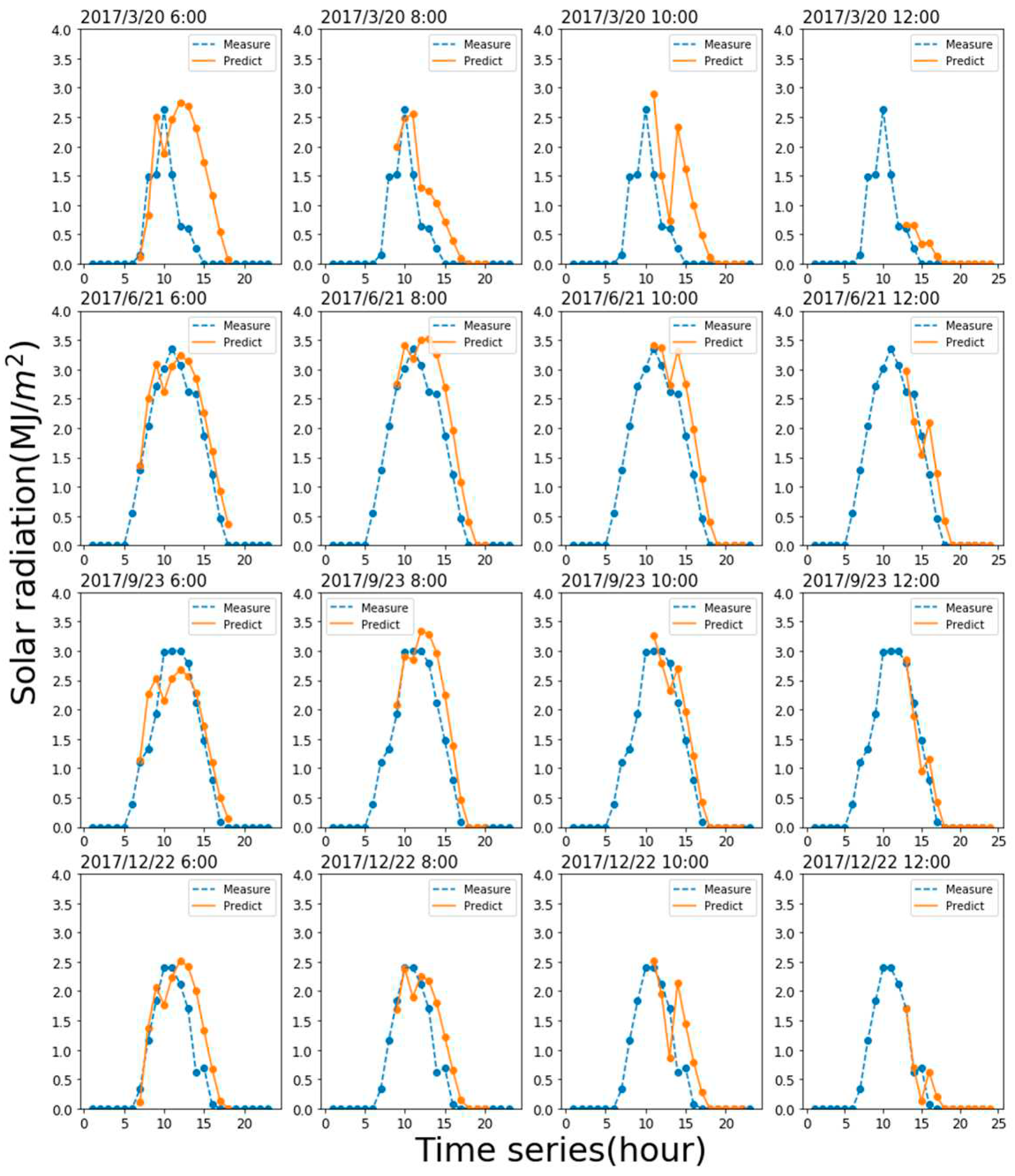
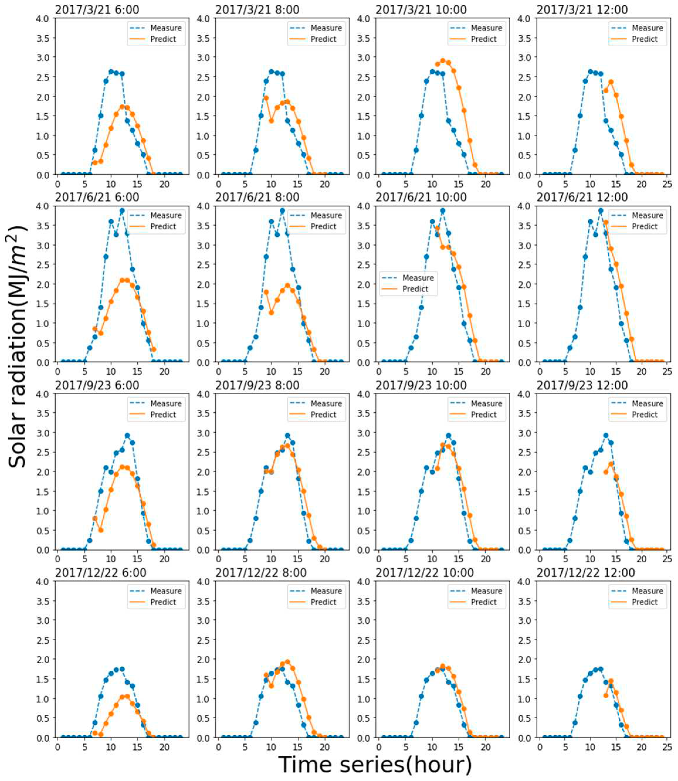
This study has established a real-time prediction system for solar radiation. The system's performance is demonstrated using representative days chosen in this study: 03/20 (spring equinox), 06/21 (summer solstice), 09/22 (autumn equinox), and 12/21 (winter solstice).
Figure 14,
Figure 15 and
Figure 16 show the real-time predictions for Kaohsiung Station, Hualien Station, and Penghu Station during these four major seasonal transitions in 2017. The orange line represents the prediction results, while the blue line represents the observed solar radiation. Each prediction starts from 6:00 AM and looks ahead to the next 12 hours. The figure titles indicate the time of the current prediction, starting at 6:00 AM, and the results are updated every two hours until noon, demonstrating the results up to that time.
It is evident that, at 6:00 AM, some stations tend to underestimate the peak around noon. However, after updating the data every two hours, by 10:00 AM, the results have significantly improved and can reasonably predict the noon peak. The results demonstrate that real-time predictions roughly align with the actual values. Based on the results, most errors are concentrated around the high values during the day. Accurate prediction of peak values can only be achieved as the current time approaches noon due to the error propagation over the long-term forecast. In such cases, the model's output becomes increasingly conservative, leading to the observed underestimation. The study suggests that using more precise cluster selection methods to accurately choose the deep neural network trained by the noon cluster could potentially resolve this underestimation issue.
6. Conclusions
The aim of this study is to establish a prediction model for solar radiation and develop a hybrid real-time solar energy prediction system to obtain reliable daily solar radiation forecasts every morning. The system is designed to provide hourly updates and corrections to the predictions, assisting in determining the future electricity generation from solar energy and the optimal timing for energy generation. The study covers three regions, namely Kaohsiung, Hualien, and Penghu, each equipped with an independent real-time prediction system, forecasting solar radiation for the next 1 to 12 hours.
In the model development phase, multiple models were employed, including the deep neural network (DNN) and the long-short term memory neural network (LSTM). Additionally, unsupervised-based algorithms were used, which involved clustering methods such as k-means clustering and fuzzy C-means clustering. After clustering the data, neural network-based prediction models were established for each cluster. As a result, in the DNN model, the following models were created: k-means DNN (k_DNN) and fuzzy C-means DNN (fc_DNN). In the case of the LSTM model, the following models were developed: k-means LSTM (k_LSTM) and fuzzy C-means LSTM (fc_LSTM).
Based on the predictions of various models, this study evaluated the best models for different forecasting time intervals and proposed a real-time solar radiation prediction system. This system is capable of providing real-time predictions for solar radiation for the range of 1 to 12 hours ahead. To test its practicality, simulations were conducted using data from the year 2017. The results of the research's prediction system demonstrated strong predictive performance. Even with increased errors in long-term predictions, the system was able to dynamically adjust the predictions in real-time, effectively forecasting solar radiation for the next 12 hours.
Author Contributions
C.-C.W. conceived and designed the experiments and wrote the manuscript, and Y.-C.Y. and C.-C.W. carried out this experiment and analysis of the data and discussed the results. All authors have read and agreed to the published version of the manuscript.
Funding
Support for this study was provided by the Ministry of Science and Technology, Taiwan under grant no. NSTC112-2622-M-019-001.
Data Availability Statement
The related data were provided by Taiwan’s Data Bank for Atmospheric Hydrologic Research, which are available at
https://dbar.pccu.edu.tw/ (accessed on 1 July 2021).
Acknowledgments
The author acknowledges the data provided by Taiwan’s Central Weather Administration.
Conflicts of Interest
The authors declare no conflict of interest.
References
- Wei, C.C.; Hsieh, P.Y. Estimation of hourly rainfall during typhoons using radar mosaic-based convolutional neural networks. Remote Sensing 2020, 12, 896. [Google Scholar] [CrossRef]
- Taipower (Taiwan Power Company). 2021. Available online: https://www.taipower.com.tw/en/index.aspx (accessed on 1 December 2021).
- Lara-Cerecedo, L.O.; Hinojosa, J.F.; Pitalúa-Díaz, N.; Matsumoto, Y.; González-Angeles, A. Prediction of the electricity generation of a 60-kW photovoltaic system with intelligent models ANFIS and optimized ANFIS-PSO. Energies 2023, 16, 6050. [Google Scholar] [CrossRef]
- Kosovic, I.N.; Mastelic, T.; Ivankovic, D. Using Artificial Intelligence on environmental data from Internet of Things for estimating solar radiation: Comprehensive analysis. Journal of Cleaner Production 2020, 266, 121489. [Google Scholar] [CrossRef]
- Makade, R.G.; Chakrabarti, S.; Jamil, B. Development of global solar radiation models: A comprehensive review and statistical analysis for Indian regions. Journal of Cleaner Production 2021, 293, 126208. [Google Scholar] [CrossRef]
- Mazzeo, D.; Herdem, M.S.; Matera, N.; Bonini, M.; Wen, J.Z.; Nathwani, J.; Oliveti, G. Artificial intelligence application for the performance prediction of a clean energy community. Energy 2021, 232, 120999. [Google Scholar] [CrossRef]
- Tsai, W.C.; Tu, C.S.; Hong, C.M.; Lin, W.M. A review of state-of-the-art and short-term forecasting models for solar PV power generation. Energies 2023, 16, 5436. [Google Scholar] [CrossRef]
- Vernet, A.; Fabregat, A. Evaluation of empirical daily solar radiation models for the northeast coast of the Iberian Peninsula. Energies 2023, 16, 2560. [Google Scholar] [CrossRef]
- Yang, X.; Ji, Y.; Wang, X.; Niu, M.; Long, S.; Xie, J.; Sun, Y. Simplified method for predicting hourly global solar radiation using extraterrestrial radiation and limited weather forecast parameters. Energies 2023, 16, 3215. [Google Scholar] [CrossRef]
- Lauret, P.; Voyant, C.; Soubdhan, T.; David, M.; Poggi, P. A benchmarking of machine learning techniques for solar radiation forecasting in an insular context. Solar Energy 2014, 112, 446–457. [Google Scholar] [CrossRef]
- Wei, C.C. Predictions of surface solar radiation on tilted solar panels using machine learning models: case study of Tainan City, Taiwan. Energies 2017, 10, 1660. [Google Scholar] [CrossRef]
- Voyant, C.; Notton, G.; Kalogirou, S.; Nivet, M.L.; Paoli, C.; Motte, F.; Fouilloy, A. Machine learning methods for solar radiation forecasting: a review. Renewable Energy 2017, 105, 569–582. [Google Scholar] [CrossRef]
- Wei, C.C. Evaluation of photovoltaic power generation by using deep learning in solar panels installed in buildings. Energies 2019, 12, 3564. [Google Scholar] [CrossRef]
- Ali, M.A.; Elsayed, A.; Elkabani, I.; Akrami, M.; Youssef, M.E.; Hassan, G.E. Optimizing artificial neural networks for the accurate prediction of global solar radiation: a performance comparison with conventional methods. Energies 2023, 16, 6165. [Google Scholar] [CrossRef]
- Chodakowska, E.; Nazarko, J.; Nazarko, Ł.; Rabayah, H.S.; Abendeh, R.M.; Alawneh, R. ARIMA models in solar radiation forecasting in different geographic locations. Energies 2023, 16, 5029. [Google Scholar] [CrossRef]
- Abumohsen, M.; Owda, A.Y.; Owda, M. Electrical load forecasting using LSTM, GRU, and RNN algorithms. Energies 2023, 16, 2283. [Google Scholar] [CrossRef]
- Bandara, K.; Bergmeir, C.; Smyl, S. Forecasting across time series databases using recurrent neural networks on groups of similar series. Expert Systems with Applications 2020, 140, 16. [Google Scholar] [CrossRef]
- Castillo-Rojas, W.; Medina Quispe, F.; Hernández, C. Photovoltaic energy forecast using weather data through a hybrid model of recurrent and shallow neural networks. Energies 2023, 16, 5093. [Google Scholar] [CrossRef]
- Cortez, B.; Carrera, B.; Jung, J.Y. An architecture for emergency event prediction using LSTM recurrent neural networks. Expert Systems with Applications 2018, 97, 315–324. [Google Scholar] [CrossRef]
- Dabiri, S.; Heaslip, K. Developing a Twitter-based traffic event detection model using deep learning architectures. Expert Systems with Applications 2019, 118, 425–439. [Google Scholar] [CrossRef]
- Li, B.; Shao, Y.; Lian, Y.; Li, P.; Lei, Q. Bayesian optimization-based LSTM for short-term heating load forecasting. Energies 2023, 16, 6234. [Google Scholar] [CrossRef]
- Petersen, N.C.; Rodrigues, F.; Pereira, F.C. Multi-output bus travel time prediction with convolutional LSTM neural network. Expert Systems with Applications 2019, 120, 426–435. [Google Scholar] [CrossRef]
- Qureshi, A.S.; Khan, A.; Zameer, A.; Usman, A. Wind power prediction using deep neural network based meta regression and transfer learning. Applied Soft Computing 2017, 58, 742–755. [Google Scholar] [CrossRef]
- Qing, X.G.; Niu, Y.G. Hourly day-ahead solar irradiance prediction using weather forecasts by LSTM. Energy 2018, 148, 461–468. [Google Scholar] [CrossRef]
- Li, G.Q.; Wang, H.Z.; Zhang, S.L.; Xin, J.T.; Liu, H.C. Recurrent Neural Networks Based Photovoltaic Power Forecasting Approach. Energies 2019, 12, 1–17. [Google Scholar] [CrossRef]
- Ghofrani, M.; Ghayekhloo, M.; Arabali, A.; Ghayekhloo, A. A hybrid short-term load forecasting with a new input selection framework. Energy 2015, 81, 777–786. [Google Scholar] [CrossRef]
- Azimi, R.; Ghayekhloo, M.; Ghofrani, M. A hybrid method based on a new clustering technique and multilayer perceptron neural networks for hourly solar radiation forecasting. Energy Conversion and Management 2016, 118, 331–344. [Google Scholar] [CrossRef]
- Reda, I.; Andreas, A. Solar position algorithm for solar radiation applications. Energy 2004, 76, 577–589. [Google Scholar]
- Hochreiter, S.; Schmidhuber, J. Long short-term memory. Neural Computation 1997, 9, 1735–1780. [Google Scholar] [CrossRef]
- Bezdek, J.C.; Ehrlich, R.; Full, W. FCM: The fuzzy c-means clustering algorithm. Computers & Geosciences 1984, 10, 191–203. [Google Scholar]
Figure 1.
Map of the study region.
Figure 1.
Map of the study region.
Figure 2.
Flowchart of a real-time prediction process.
Figure 2.
Flowchart of a real-time prediction process.
Figure 3.
The modeling process for DNN models.
Figure 3.
The modeling process for DNN models.
Figure 4.
Figure 4. Input-output pattern used in DNN model.
Figure 4.
Figure 4. Input-output pattern used in DNN model.
Figure 5.
The concept of network structures in RNN and LSTM models.
Figure 5.
The concept of network structures in RNN and LSTM models.
Figure 6.
Figure 6. Input-output patterns in LSTM model.
Figure 6.
Figure 6. Input-output patterns in LSTM model.
Figure 7.
The modeling process for unsupervised combined with supervised models.
Figure 7.
The modeling process for unsupervised combined with supervised models.
Figure 8.
Procedure of the data samples clustering.
Figure 8.
Procedure of the data samples clustering.
Figure 9.
Error convergence trends over iterations for SGD versus Adam optimizer.
Figure 9.
Error convergence trends over iterations for SGD versus Adam optimizer.
Figure 10.
Calibration of delay time d of DNN model in (a) Kaohsiung Station, (b) Hualien Station, (c) Penghu Station.
Figure 10.
Calibration of delay time d of DNN model in (a) Kaohsiung Station, (b) Hualien Station, (c) Penghu Station.
Figure 11.
Calibration of neuron nodes in LSTM: (a) Kaohsiung Station, (b) Hualien Station, (c) Penghu Station.
Figure 11.
Calibration of neuron nodes in LSTM: (a) Kaohsiung Station, (b) Hualien Station, (c) Penghu Station.
Figure 12.
Calibration of clustering amount in cluster-based DNN and LSTM models in (a) Kaohsiung Station, (b) Hualien Station, (c) Penghu Station.
Figure 12.
Calibration of clustering amount in cluster-based DNN and LSTM models in (a) Kaohsiung Station, (b) Hualien Station, (c) Penghu Station.
Figure 13.
The results of rRMSE using testing set: (a) Kaohsiung; (b) Hualien; (c) Penghu.
Figure 13.
The results of rRMSE using testing set: (a) Kaohsiung; (b) Hualien; (c) Penghu.
Figure 14.
Real-time prediction system simulation results for Kaohsiung Station.
Figure 14.
Real-time prediction system simulation results for Kaohsiung Station.
Figure 15.
Real-time prediction system simulation results for Hualien Station.
Figure 15.
Real-time prediction system simulation results for Hualien Station.
Figure 16.
Real-time prediction system simulation results for Penghu Station.
Figure 16.
Real-time prediction system simulation results for Penghu Station.
Table 1.
Statistics of ground-level climate attributes.
Table 1.
Statistics of ground-level climate attributes.
| Attribute |
Unit |
Min−Max, Mean |
| Kaohsiung Station |
Hualien Station |
Penghu Station |
| Atmospheric pressure |
hPa |
976.1−1030.9, 1012.0 |
958.8−1032.1, 1011.8 |
974.1−1033, 1011.8 |
| Surface temperature |
°C |
7.1−36.9, 25.31 |
9.2−39.6, 24.66 |
7.9−34.8, 23.67 |
| Dew temperature |
°C |
-4.2−30.4, 20.49 |
1.5−29.2, 19.64 |
-0.4−29.8, 19.95 |
| Relative humidity |
% |
26−100, 75.24 |
25−100, 74.21 |
27−100, 80.12 |
| Water vapor |
hPa |
4.5−43.4, 24.93 |
6.8−40.5, 23.65 |
5.9−41.9, 24.34 |
| Average wind speed |
m/s |
0−18, 2.17 |
0−16.6, 1.74 |
0−25.8, 4.06 |
| Precipitation |
mm |
0−119.5, 0.21 |
0−83, 0.21 |
0−94.5, 0.13 |
| Rainfall duration |
h |
0−1, 0.04 |
0−1, 0.06 |
0−1, 0.05 |
| Insolation duration |
h |
0−1, 0.26 |
0−1, 0.20 |
0−1, 0.24 |
| Global solar radiation |
MJ/m2
|
0−3.90, 0.56 |
0−5.32, 0.63 |
0−4.34, 0.53 |
| Declination angle |
degree |
-23.45−23.45, -0.01 |
-23.45−23.45, -0.01 |
-23.45−23.45, -0.01 |
| Hour angle |
degree |
-165−180, 7.5 |
-165−180, 7.5 |
-165−180, 7.5 |
| Zenith angle |
degree |
0.02−179.98, 90 |
0.028−179.97, 90 |
0.12−179.88, 90 |
| Elevation angle |
degree |
-89.98−89.98, 0.0 |
-89.97−89.97, -0.0 |
-89.88−89.88, 0.0 |
| Azimuth angle |
degree |
-90−90, 0.0 |
-90−90, 0.0 |
-90−90, 0.0 |
Table 2.
Parameter tuning results for the DNN model.
Table 2.
Parameter tuning results for the DNN model.
| Station |
Delay time (h) |
Number of hidden layers |
Number of neuron nodes |
RMSE (MJ/m2) |
| Kaohsiung |
7 |
3 |
18 |
0.232196 |
| Hualien |
10 |
3 |
10 |
0.262571 |
| Penghu |
5 |
3 |
9 |
0.232947 |
|
Disclaimer/Publisher’s Note: The statements, opinions and data contained in all publications are solely those of the individual author(s) and contributor(s) and not of MDPI and/or the editor(s). MDPI and/or the editor(s) disclaim responsibility for any injury to people or property resulting from any ideas, methods, instructions or products referred to in the content. |
© 2023 by the authors. Licensee MDPI, Basel, Switzerland. This article is an open access article distributed under the terms and conditions of the Creative Commons Attribution (CC BY) license (http://creativecommons.org/licenses/by/4.0/).
