0. Introduction
In today's intensive, large-scale pig farming environment, intelligent farming has received more and more attention and research, machine instead of manpower has become the development trend of efficient farming, but also the inevitable trend of the development of intelligent farming [
1]. At present, machine vision, deep learning, Internet of Things, artificial intelligence and other technologies have been applied in the cleaning, inspection, feeding, and epidemic prevention and control of swine farms robots to liberate the labour force [
2,
3,
4,
5], improve production efficiency while reducing the risk of disease transmission between humans and animals, showing great application value and development prospects [
6]. Navigation and positioning is the core technology of robots, satellite signals can not cover the indoor pig farms, high-precision indoor positioning technology is of great significance to the breeding robots.
Ultra Wideband (UWB) positioning has the advantages of low system complexity, strong anti-jamming, high transmission rate, low energy consumption, positioning and ranging accuracy can reach the decimetre or even centimetre level [
7], which is suitable for the positioning of breeding robots in pig farms. Through the deployment of positioning BTS in the farm, the robot is equipped with positioning tags, which can help the staff in front of the host computer to determine the position of the robot. The accuracy of the tag position does not only depend on the localisation algorithm, but is also related to the height at which the positioning BTS are deployed, the spacing between the BTS and the shape of the deployment. Dilution of precision (DOP) is an important parameter to measure the positioning accuracy, it can assess the relative geometric relationship on the ranging error and positioning accuracy, in the same base station equivalent distance error conditions, the smaller the DOP value, the higher the positioning accuracy [
8]. Root-Mean-Square Error (RMSE) is the square root of the difference between the observed value and the true value, which is used to measure the positioning error, the smaller the RMSE value, the smaller the error, which is used to evaluate the position estimation accuracy of UWB indoor positioning tag [
9]. Variance (variance) is used to measure the degree of dispersion of the positioning data.
By studying the principles and methods of base station deployment, it achieves the position settlement of the positioning base station to the positioning tags, optimises the BTS deployment scheme, improves the positioning accuracy and stability, and provides a guarantee for the high-precision positioning of the breeding robots in pig farms. The literature introduces the concept and types of accuracy factors and their relationship with positioning accuracy, and investigates the effect of base station geometry on positioning accuracy [
10,
11].
A study through the GDOP analysis of the results of following positioning of mobile devices at different locations in a circular area, the expression is compared with the simulation results, and the resolved positioning in the closed area surrounded by away from the base station and the base station matches well with the simulation results, which provides a reference for the design and testing of precise positioning and following positioning [
12]. Guo Y found that even if the ranging error is small, the localisation error is large in a narrow space, thus a localisation algorithm combining Kalman filtering (KF) and precision factor (DOP) is proposed to improve the accuracy and stability of localisation in a narrow space [
13]. Albaidhani A proposed a positioning algorithm suitable for indoor use and tested the UWB positioning system under this algorithm using the values of the mean square error (MSE) and the factor of precision (DOP) to select the optimal base station placement and improve the positioning accuracy [
14].The study by calculating and simulating the positioning accuracy factor under different numbers of pseudo-satellites, the optimal observation matrix was calculated using matrix eigenvalue analysis, and the four-satellite layout was calculated as the optimal observation matrix [
15]. Taking different types of accuracy factors as the theoretical basis, he proposed the establishment of a four-dimensional model with altitude angle, azimuth angle and observation time as independent variables and relative accuracy factor as dependent variable to improve the accuracy of positioning and provide a guarantee for the optimal deployment of satellites [
16]. Through experiments comparing and analysing the positioning trajectories and real trajectories of different factors, it is concluded that UWB dynamic positioning will be affected by the position of positioning tags, travelling speed, pedestrian interference, and the highest accuracy of positioning the centre of the BTS area [
17].The study by analysing the distribution of the accuracy factor of different deployment schemes through real and simulated positioning experiments, it is concluded that the accuracy factor of the test points will be affected by factors such as the regional scope, number and height of the positioning BTS deployment, and that the terminal positioning accuracy can be improved when the number of BTS and the height angle of the test points and the BTS are reasonably increased inside the closed area surrounded by the BTS [
18].
1. UWB Positioning Principles
The UWB positioning system selected in this paper adopts Time of Arrival (TOA), which is based on the estimation of the time delay from the node to be located to the reference BTS, so as to obtain the distance from the BTS to the location. The advantage of the TOA positioning method is that it can make full use of the characteristics of the ultra-wideband signal with a high time division rate to detect the time delay of the signal on the receiving end, so that the distance from the node to be located to the reference BTS can be estimated. The distance from the node to be located to the reference BTS is estimated, and then the coordinates of the node to be located can be calculated according to the basic UWB positioning algorithm. The positioning model of TOA positioning in three-dimensional space is a spherical model, which requires at least four BTS. The positioning accuracy is also closely related to the precise clock synchronisation between BTS.
The coordinate of
jth BTS is
. Solving for label coordinates
. Assuming the synchronisation condition i.e. no clock difference, when there are
n measured values,
represent the distance between tag and
jth BTS
L as a measured value which can be expressed as:
According to Taylor’s theorem:
The partial derivative at
is:
Assume
as the cosine of the direction of the coordinates solved by the positioning algorithm with respect to the BTS coordinates
j:
Where
is the vector of offset of the true position of the tag from the positioning algorithm solver,
is the vector offset of the true range to the range values corresponding to the linearization point.
According to the Ordinary Least Square (OLS)
dx is the position error,
dr is the range measurement error
The covariance of
dx is:
In the measurements the errors are random, independent, in zero mean and the rms in common.
is the Root Mean Square (
rms), the Error Covariance Matrix is:
The Matrix of weight coefficients
I is:
2. Positioning results assessment
DOP、HDOP、VDOP、PDOP are an important basis for evaluating positioning results [
11,
12,
19,
20].
DOP(Dilution Of Precision)defined as:
HDOP(Horizontal Dilution Of Precision)
VDOP(Vertical Dilution Of Precision)
PDOP(Position Dilution Of Precision)
GDOP(Geometric Dilution Of Precision)
3. Experimental analyses
For the reasonable analysis of pig farm positioning environment, generally in the pig farm corridor or the wall of the pig farm for the installation of positioning BTS deployment, this paper sets up a variety of BTS deployment scheme, the DOP value as a measure, through the simulation of positioning experiments and real positioning experiments, to analyse the impact of UWB positioning BTS deployment on the positioning results. The height of the positioning terminal is 100cm.
3.1. Simulation and analysis
3.1.1. Different height of BTS
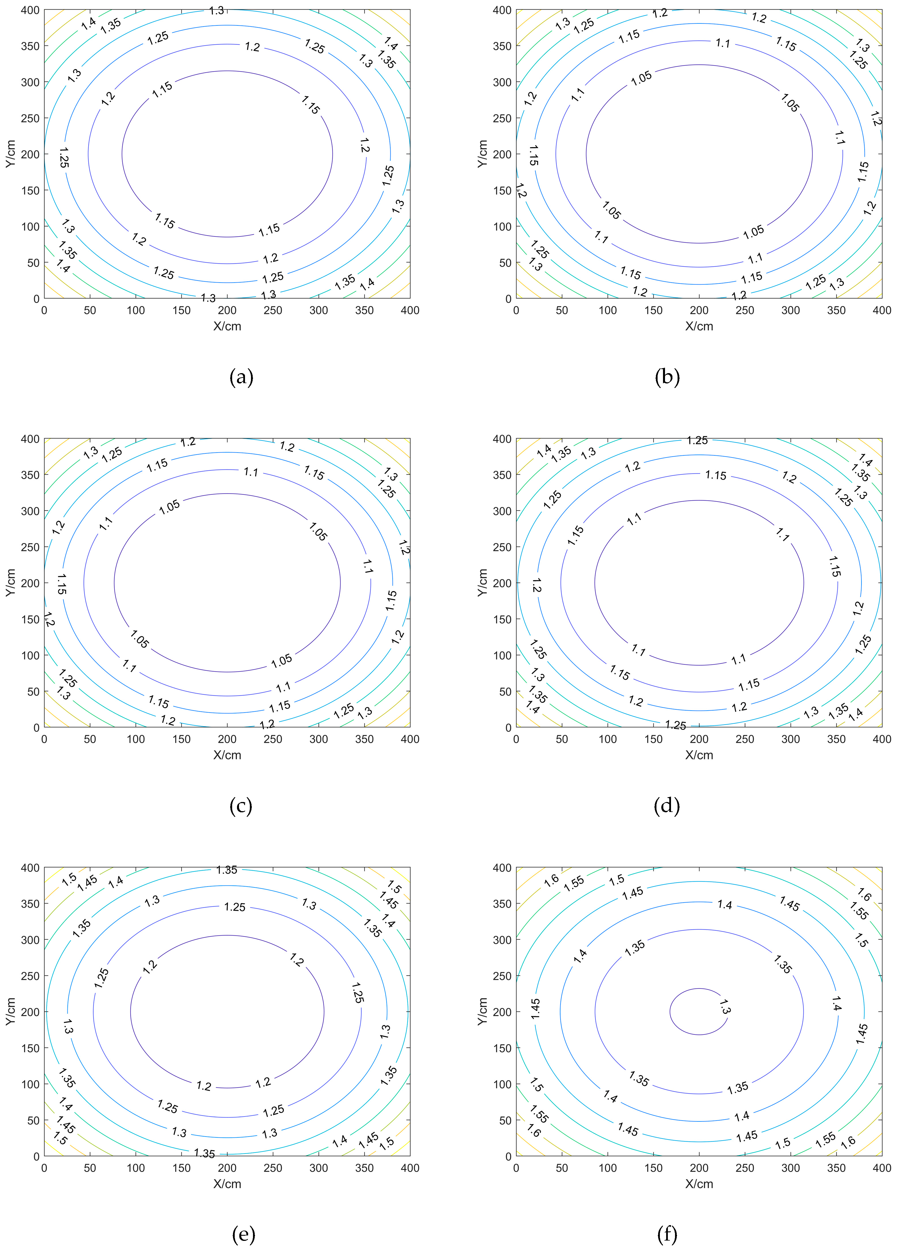
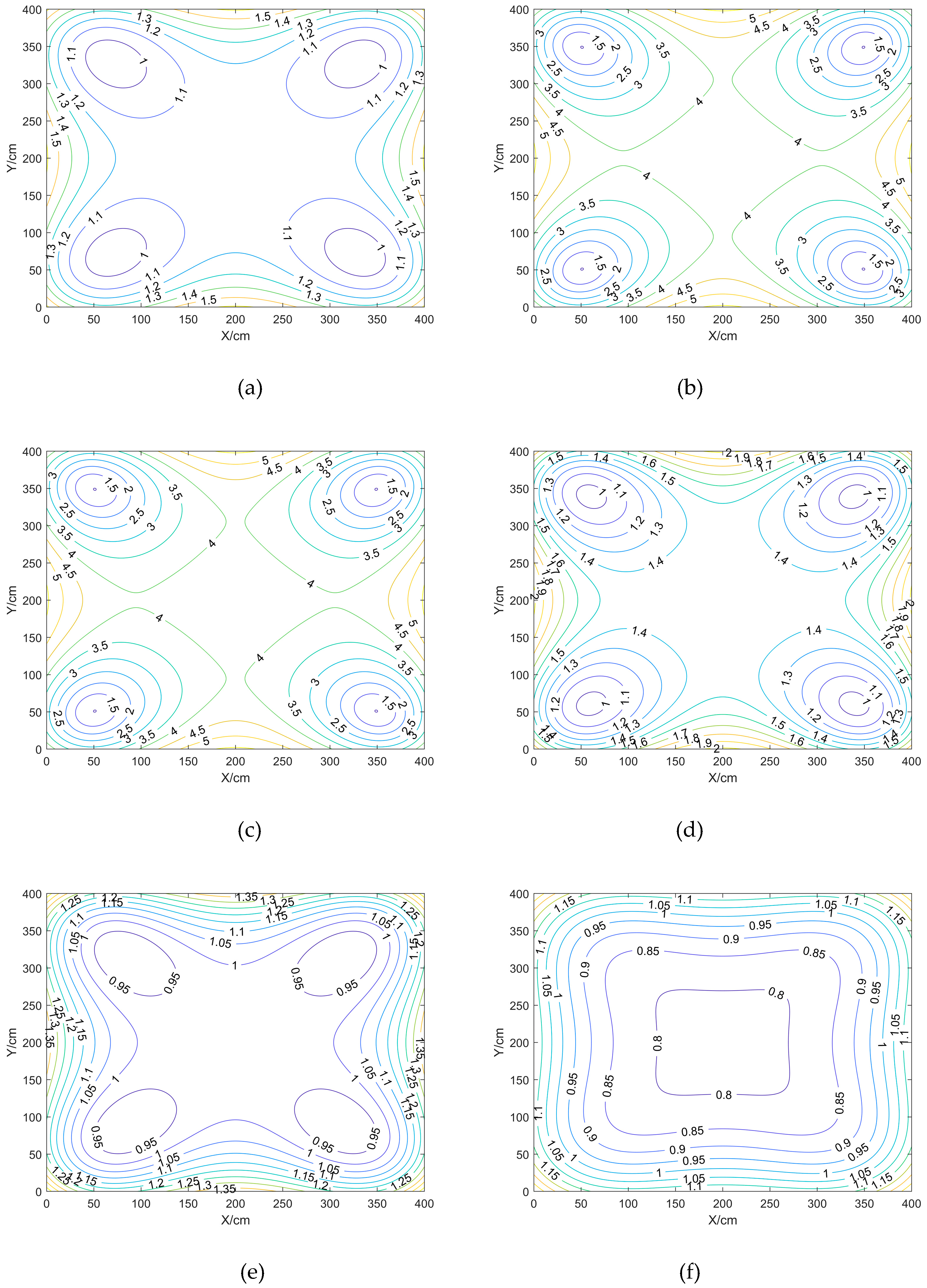
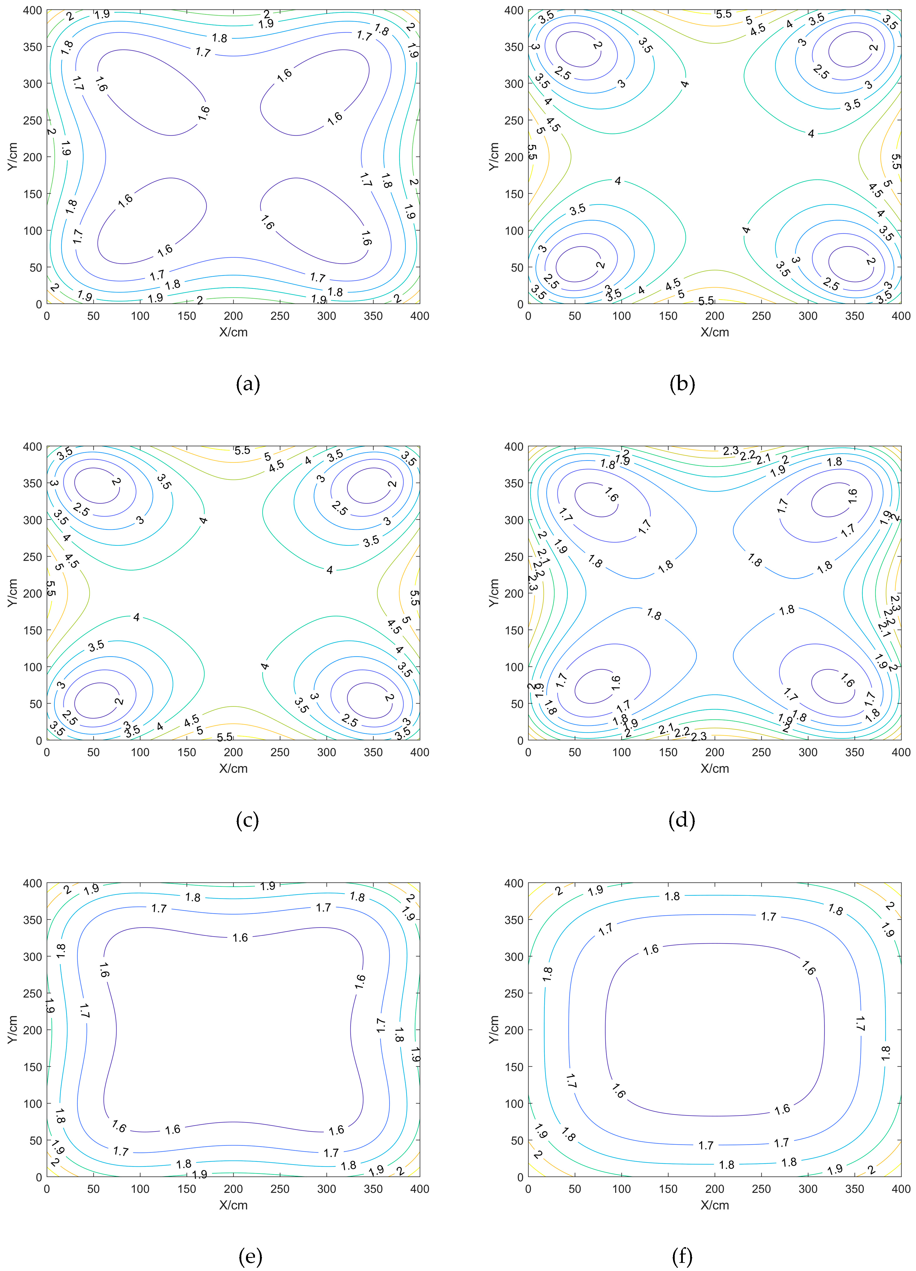
Comparison and analysis of the effect of different BTS heights on positioning accuracy in the case of fixed BTS spacing and BTS deployment shape, with BTS heights set to 0 cm, 75 cm, 125 cm, 175 cm, 225 cm, 275 cm, respectively.
Table 1.
The BTS coordinates at different heights.
Table 1.
The BTS coordinates at different heights.
| BTS deployment programme |
A0
|
A1
|
A2
|
A3
|
| a |
(50,50,0) |
(50,350,0) |
(350,350,0) |
(350,50,0) |
| b |
(50,50,75) |
(50,350,75) |
(350,350,75) |
(350,50,75) |
| c |
(50,50,125) |
(50,350,125) |
(350,350,125) |
(350,50,125) |
| d |
(50,50,175) |
(50,350,175) |
(350,350,175) |
(350,50,175) |
| e |
(50,50,225) |
(50,350,225) |
(350,350,225) |
(350,50,225) |
| f |
(50,50,275) |
(50,350,275) |
(350,350,275) |
(350,50,275) |
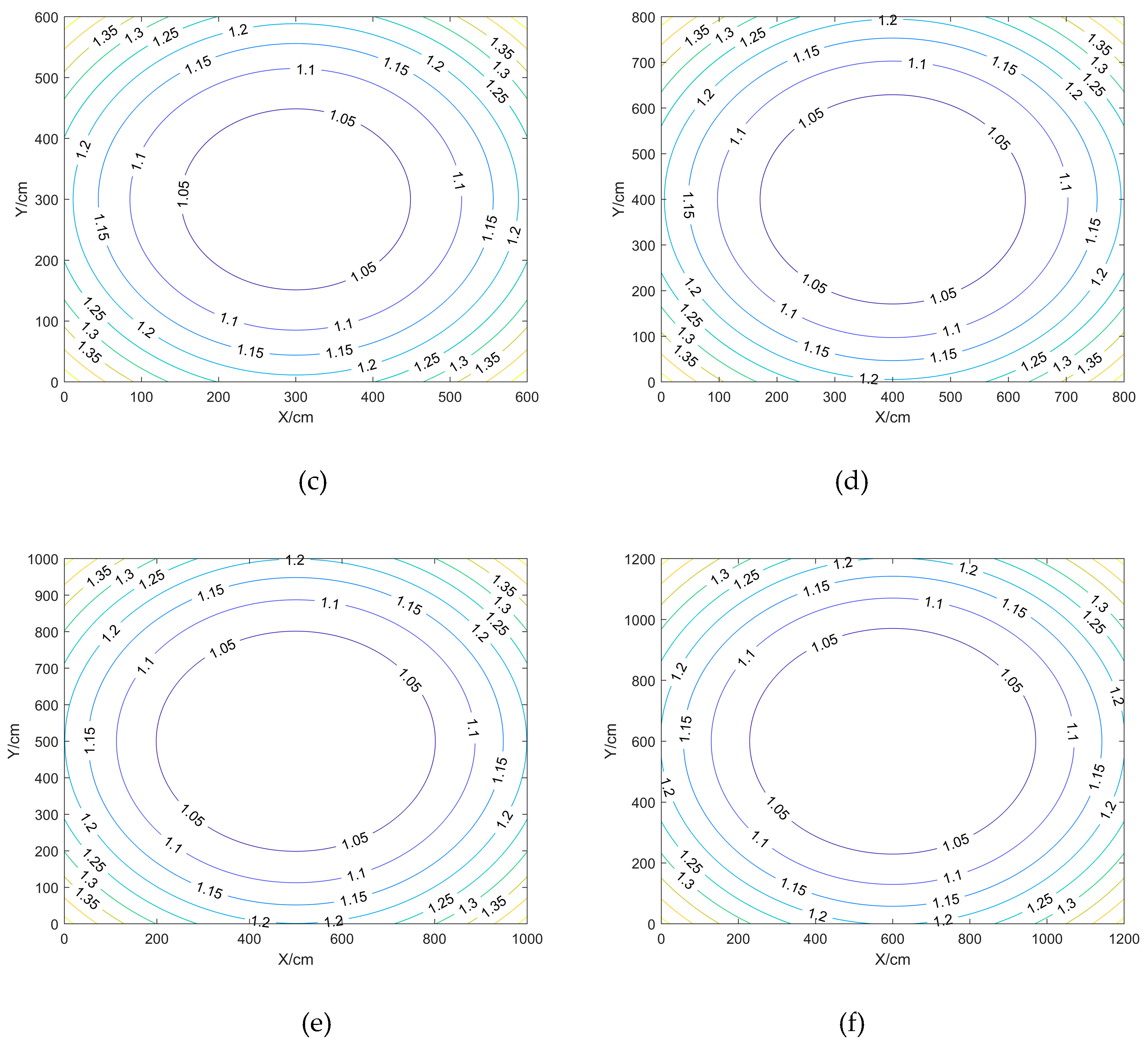
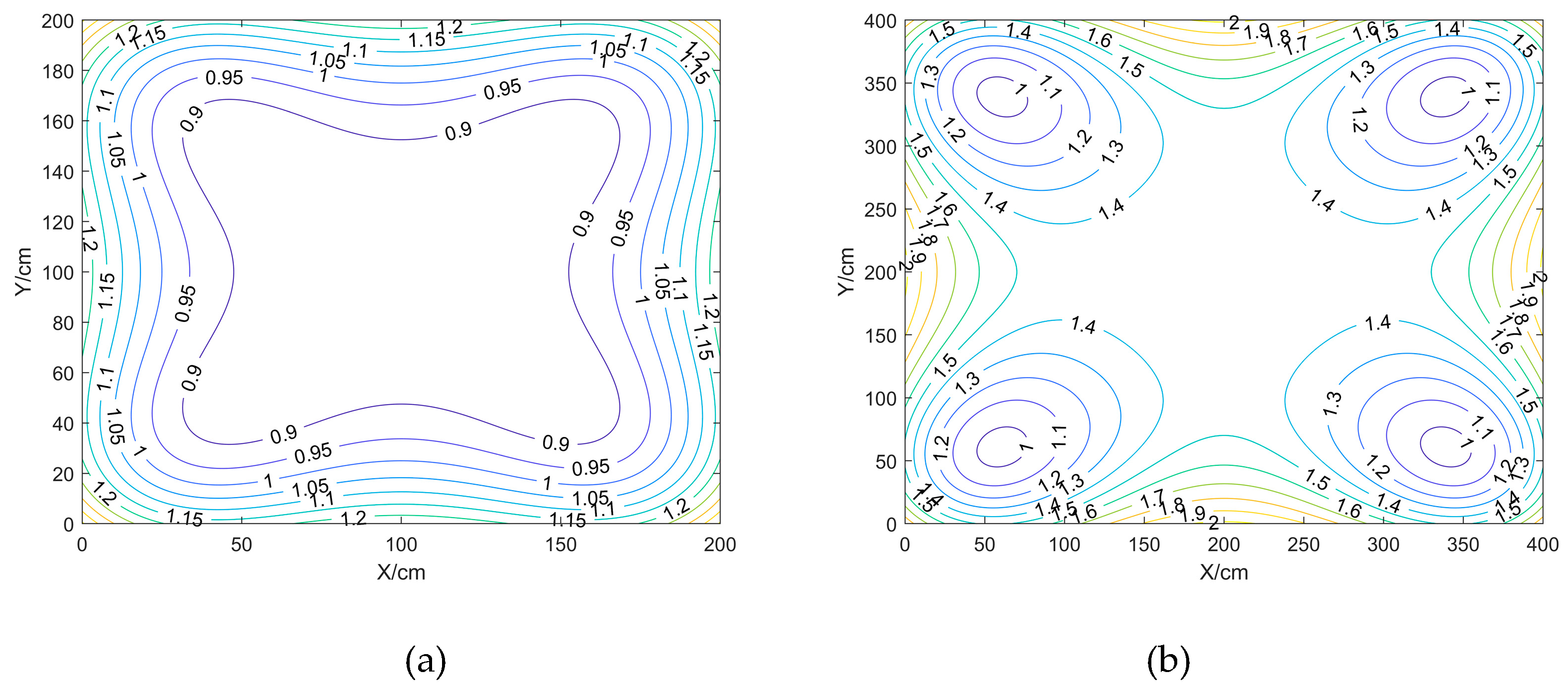
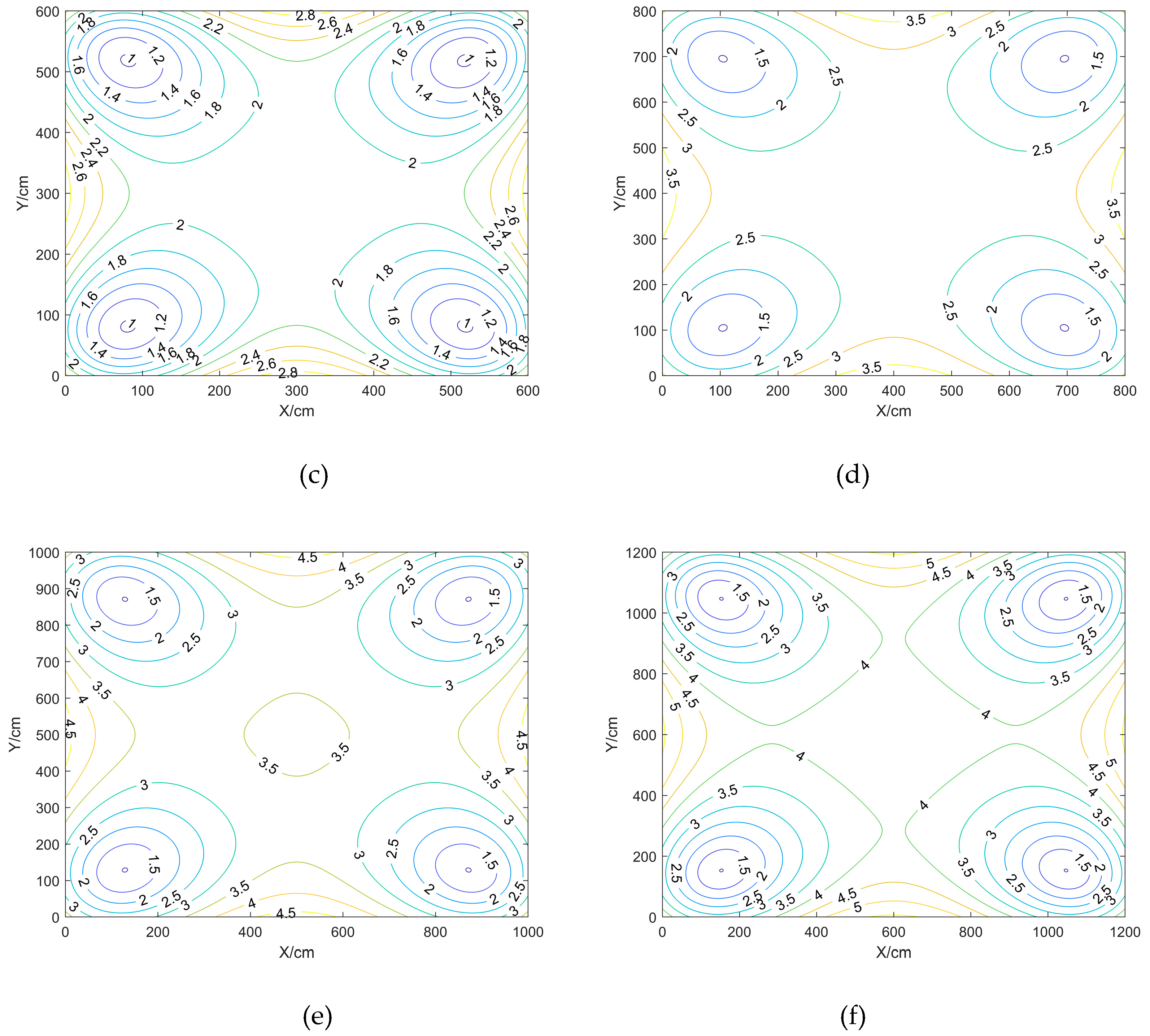
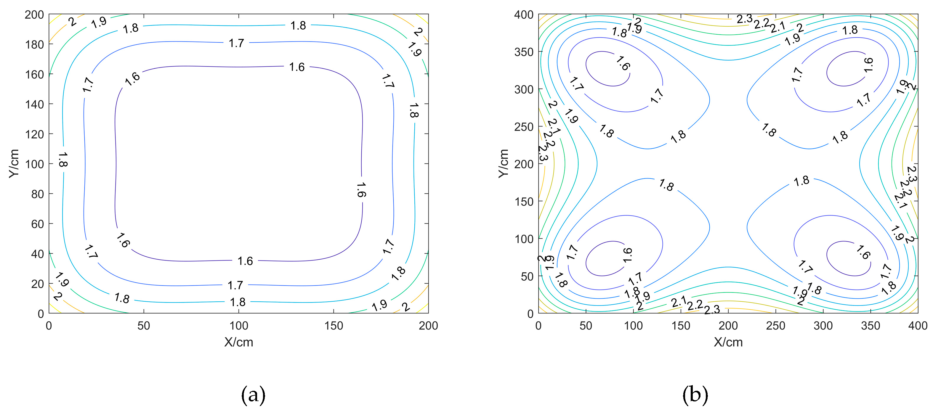
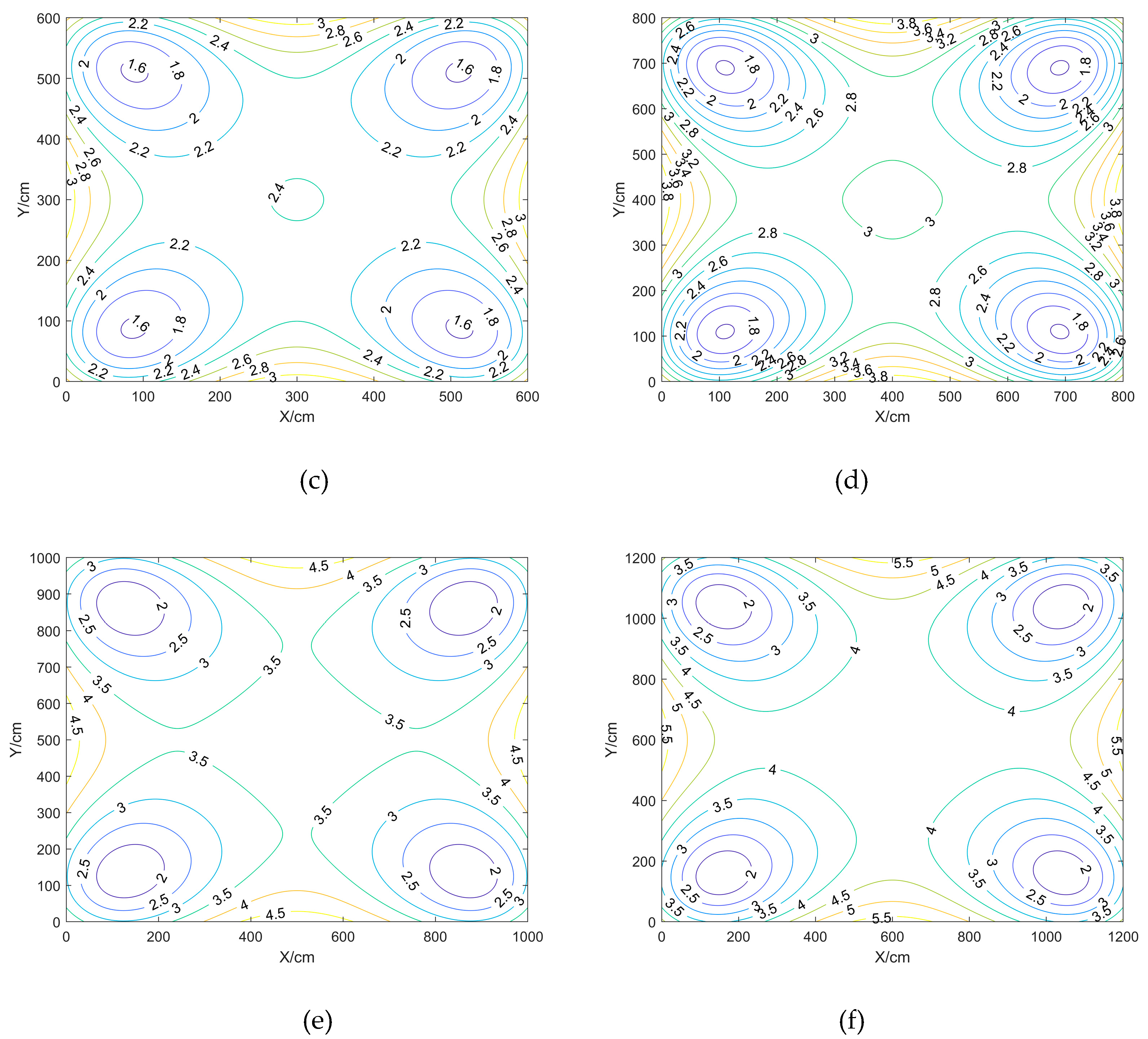
Inside the closed area enclosed by the BTS: the HDOP value near the centre point location is smaller, while the VDOP and PDOP values will be larger; the VDOP and PDOP near the BTS are smaller, and the values near the centre point location will be larger;
Outside the closed area surrounded by the BTS: the further out the DOP values are all larger.
This can be obtained through
Table 2:
Scenario a and b have equal maximum, minimum and average DOP values, compared to the other scenarios, HDOP has the smallest maximum, minimum and average values, and VDOP and PDOP have the largest maximum, minimum and average values; Scenarios f have the largest maximum, minimum and average values of HDOP, and vice versa for VDOP and PDOP. the maximum, minimum and average values of HDOP for the scenarios differ from each other by no more than 0.3, whereas the maximum values of VDOP and PDOP differ more between Scenarios b and c and the other scenarios, and the minimum values differ less.
In summary, when the shape and spacing of the BTS arrangement are fixed, the difference in height between the BTS and the positioning point can be adjusted appropriately to reduce the DOP value, the higher the BTS is, the larger the HDOP value will be, and the smaller the VDOP and PDOP values will be, and the appropriate height of the BTS is between 175 and 275.
3.1.2. Different distance of BTS
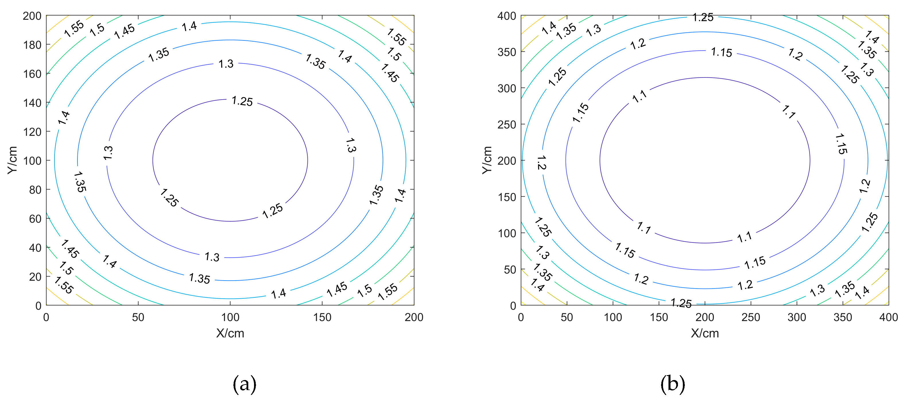
Comparison and analysis of the effect of different spacing of BTS on positioning accuracy in the case of BTS height of 175cm and fixed square shape of BTS deployment, the spacing of BTS deployment are: 150, 300, 450, 600, 750, 900 square, respectively.
Table 3.
BTS deployment programme when BTS spacing is different.
Table 3.
BTS deployment programme when BTS spacing is different.
| BTS deployment programme |
A0
|
A1
|
A2
|
A3
|
| a |
(25,25,175) |
(25,175,175) |
(175,175,175) |
(175,25,175) |
| b |
(50,50,175) |
(50,350, 175) |
(350,350,175) |
(350,50,175) |
| c |
(75,75,175) |
(75,525, 175) |
(525,525,175) |
(525,75,175) |
| d |
(100,100,175) |
(100,700,175) |
(700,700,175) |
(700,100,175) |
| e |
(125,125,175) |
(125,875,175) |
(875,875,175) |
(875,125,175) |
| f |
(150,150,175) |
(150,1050,175) |
(350,1050,175) |
(1050,150,175) |
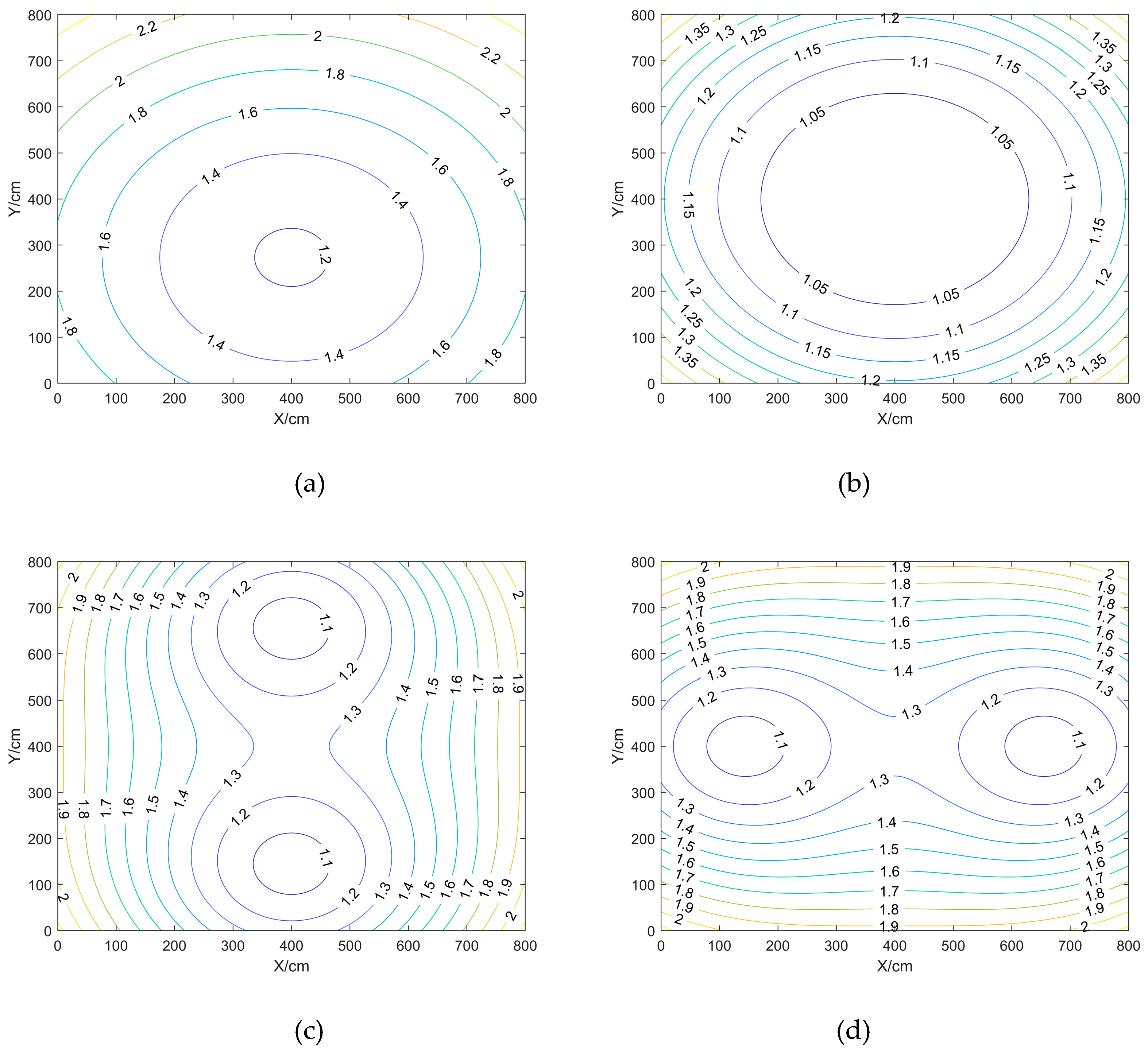
Inside the square area enclosed by the BTS: the closer to the centre point position the smaller the HDOP value is, and the larger the VDOP and PDOP values are; the closer to the BTS the smaller the VDOP and PDOP values are, and the closer to the centre point position the larger the VDOP and PDOP values are;
Outside the enclosed area surrounded by the BTS, the further out the DOP values are larger.
This can be obtained through
Table 4:
As the side length of the BTS gets bigger and bigger, the HDOP value decreases gradually, and the VDOP and PDOP values increase gradually; for Scenarios f, the maximum, minimum, and average values of HDOP are the smallest, and the maximum and average values of VDOP and PDOP are the largest, but the minimum values of VDOP and PDOP for the six scenarios are basically the same;
Summary can be obtained: when the BTS height and layout shape is fixed, appropriate adjustment of the BTS spacing can reduce the DOP value, the larger the range of the BTS, the HDOP maximum and minimum values will be smaller, VDOP and PDOP minimum value does not change much, the BTS spacing in 150cm DOP value is relatively large, the spacing of the range of 300cm and above is better.
3.1.3. Different Shape of BTS arrangements
Comparison and analysis of the effect of different shapes of BTS layout on positioning accuracy in the case of fixed BTS spacing and BTS height, the BTS layout is set up as an equilateral triangle with a side length of 600cm, a square with a side length of 600cm, a rectangle with a length of 600cm and a width of 300cm, and a rectangle with a length of 300cm and a width of 600cm, respectively.
Table 5.
BTS deployment plan for different shapes.
Table 5.
BTS deployment plan for different shapes.
| BTS deployment programme |
A0
|
A1
|
A2
|
A3
|
| a |
(100,100,175) |
(400,619.6,175) |
|
(700,100,175) |
| b |
(100,100,175) |
(100,700,175) |
(700,700,175) |
(700,100,175) |
| c |
(100,250,175) |
(100,550,175) |
(700,550,175) |
(700,250,175) |
| d |
(250,100,175) |
(250,700,175) |
(550,700,175) |
(550,100,175) |
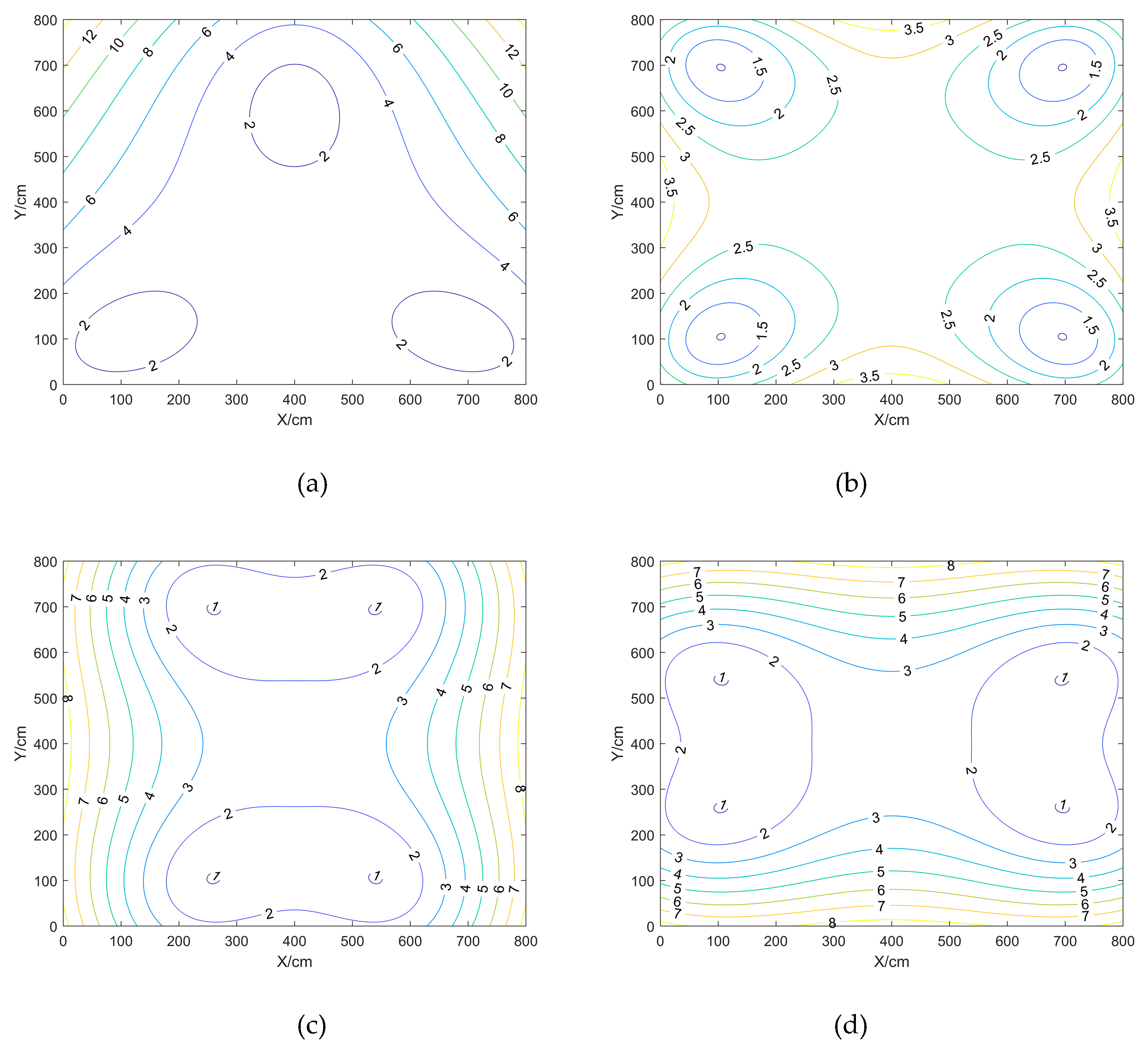
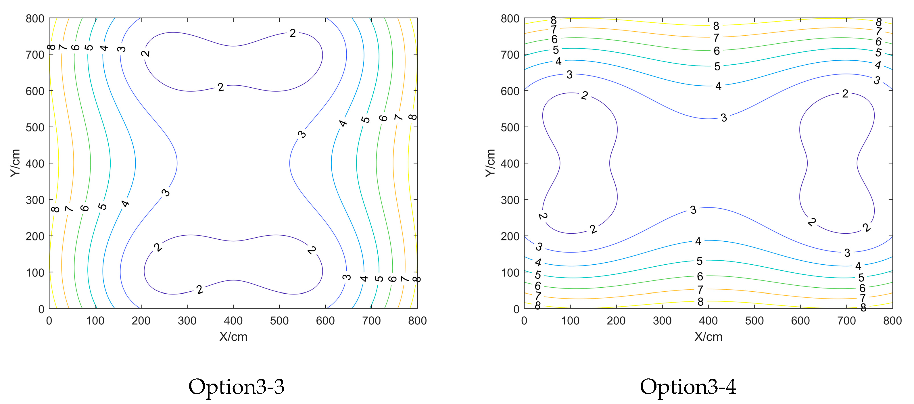
Inside the closed area enclosed by the BTS: the HDOP values are smaller near the centre point location and larger near the BTS; the VDOP and PDOP values are smaller near the BTS;
Outside the closed area surrounded by the BTS, the DOP values are larger, and the further out the DOP values are all larger.
This can be obtained through
Table 6:
Scenario b, when the BTS is laid out as a square, the DOP value is the smallest. Scenario 1, when the equilateral triangle, the DOP value is the largest, and when the aspect ratio of rectangles is the inverse of each other, the DOP values are the same.
In summary, it can be concluded that: when the BTS is deployed as a square, the DOP value is the smallest, and the positioning effect is the best, and the rectangle is the second, when the BTS is deployed as a rectangle, the DOP value of the long side is smaller than that of the short side, i.e., the accuracy of the long side is high.
3.2. Analysis of real measurement experiments
The real-world experiments were conducted using LinkTrack P-A module hardware, divided into static fixed-point localisation and dynamic following localisation, in an open field with no interfering objects in the area enclosed by the BTS, and the size of the test site was adjusted according to the variables required for the experiments.
3.2.1. Static positioning analysis
For the square quadrilateral area surrounded by 4 BTS, points were taken near 75cm of the BTS, the midpoint of the two BTS and the midpoint of the quadrilateral, with a total of 13 points; for the square trilateral area surrounded by 3 BTS, points were taken near 75cm of the BTS, the midpoint of the two BTS and the midpoint of the trilateral, with a total of 10 points. Each fixed point was sampled within 3 minutes, and the sampling frequency was 10 HZ.
Different height of BTS
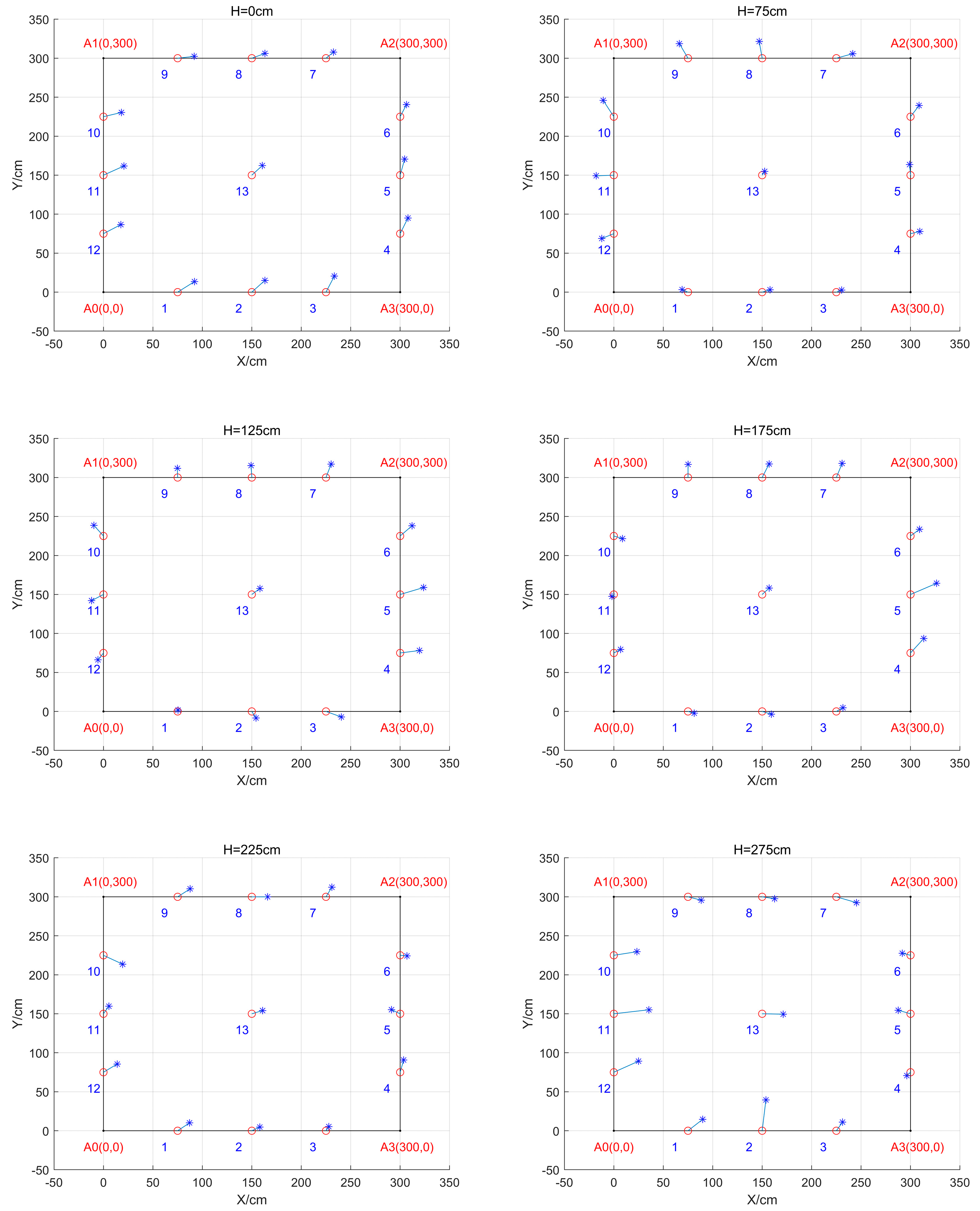
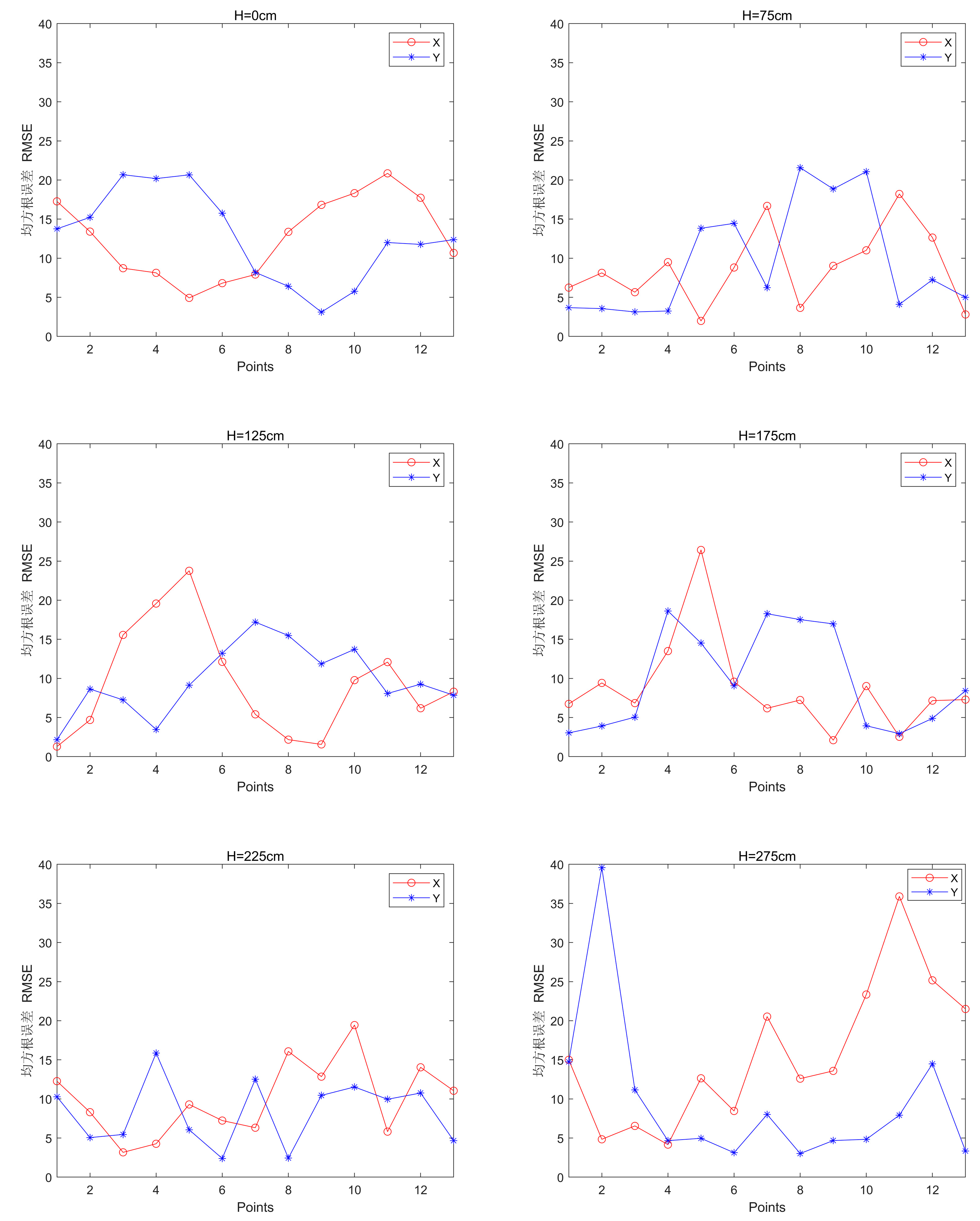
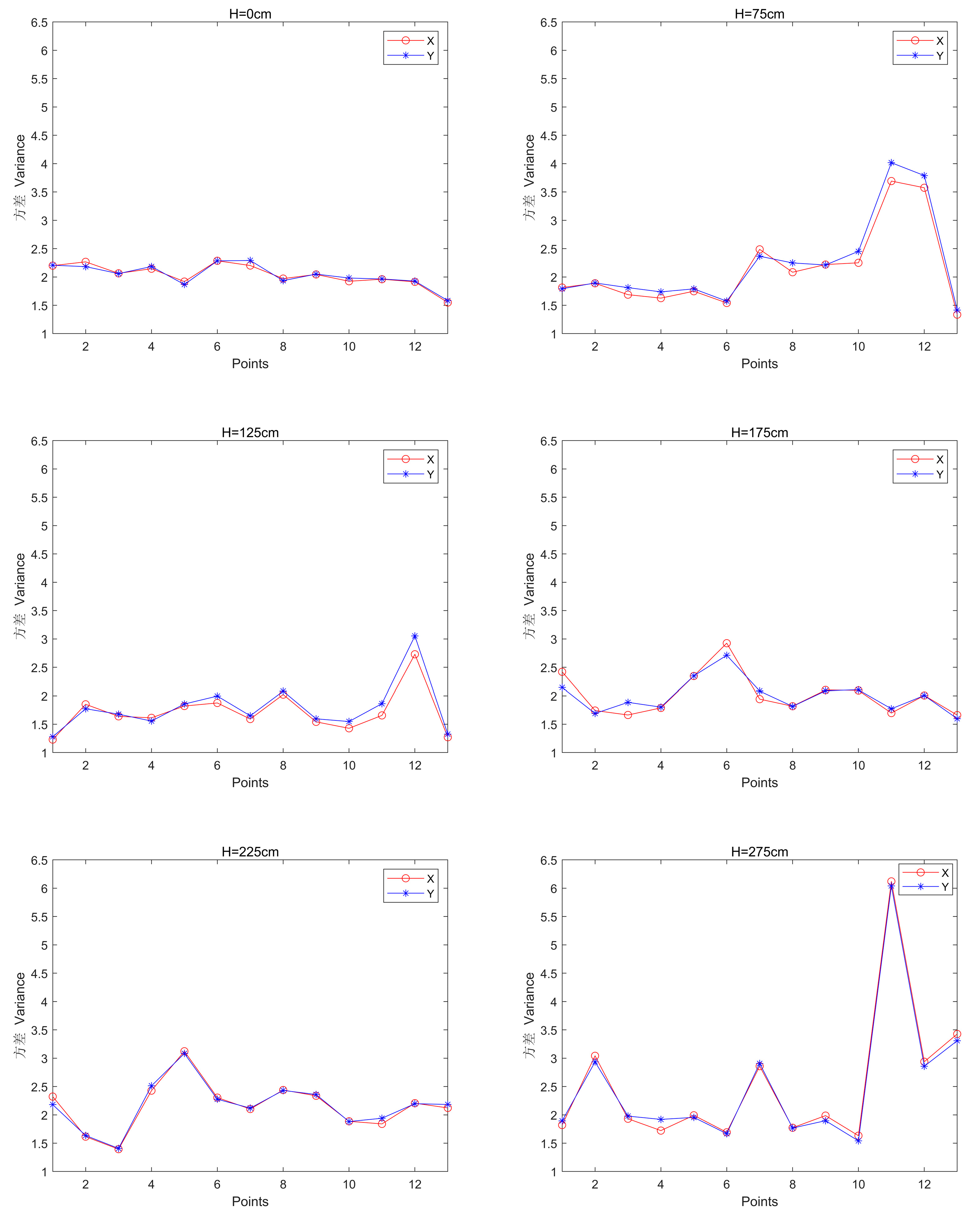
The BTS is a square with a spacing of 300cm and the UWB positioning effect when the height of the BTS is set to 0cm, 75 cm, 125 cm, 175 cm, 225 cm and 275 cm respectively.
Figure 10,
Figure 11 and
Figure 12 can be obtained: when H=0 and 275, the deviation of each point is larger; when H=175 and 225, the deviation is smaller, and the root-mean-square error is within 15 for more points; when H=125 and 175, the variance is smaller for both, and within 2 for more points; when H=275, the variance is larger for more points. The same height and point location is that the X and Y coordinate variances are approximate.
Table 7 can be obtained: H = 75, X maximum value and the average value of the smallest, H = 125, X minimum value of the smallest, H = 0 X minimum value of the largest, H = 275 average value of the largest; H = 225, Y maximum value of the smallest, H = 125, Y minimum value, the average value of the smallest, H = 275 Y maximum value, the average value of the largest, H = 0, Y minimum value of the smallest.
Table 8 can be obtained: when H=0, X maximum value and average value is minimum, when H=125, X minimum value is minimum, when H=275, X maximum value and average value is maximum, when H=175, X minimum value is maximum; when H=0, Y maximum value and average value is minimum, when H=125, Y minimum value is minimum, when H=275, Y maximum value, average value is maximum and Y minimum value is maximum. The difference between X and Y variance values at the same point in the same height case is not significant.
Different distance of BTS
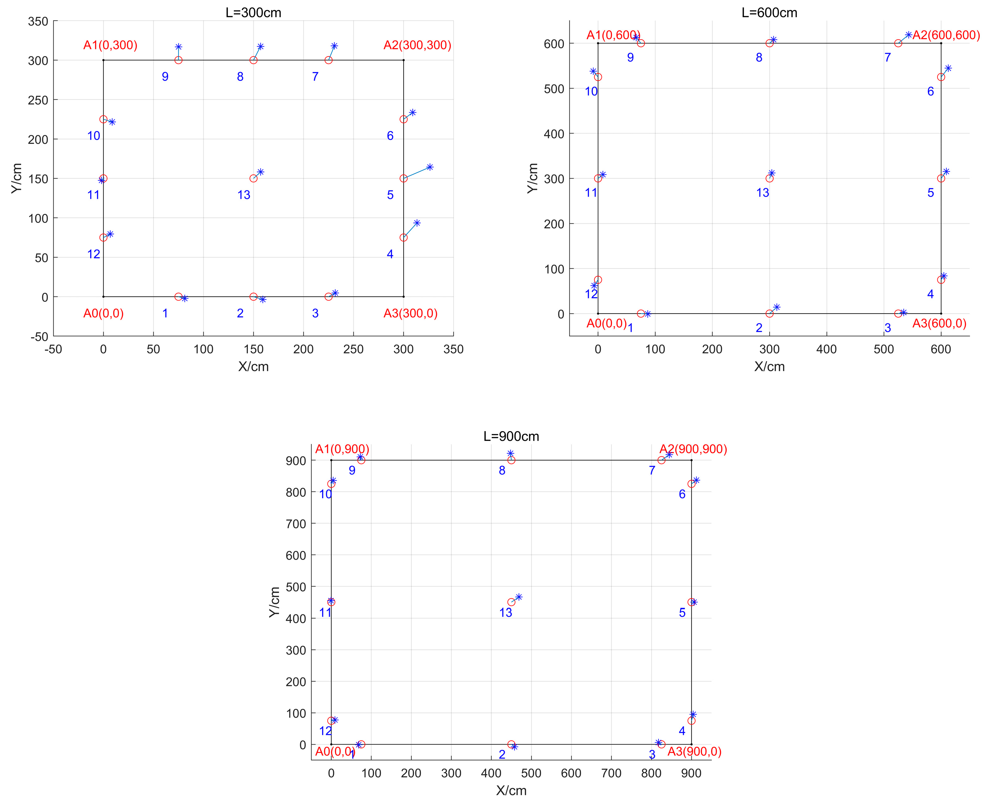
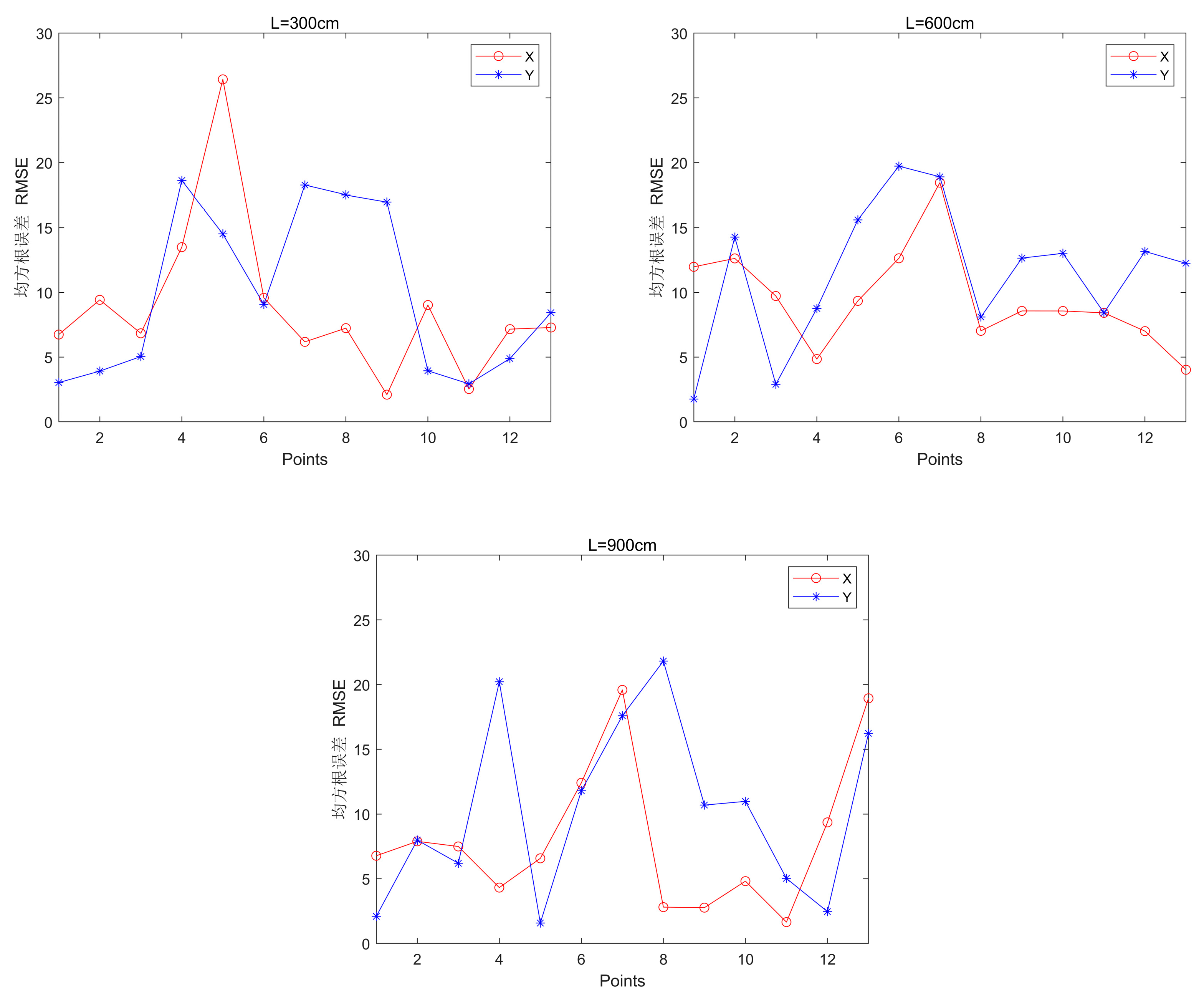
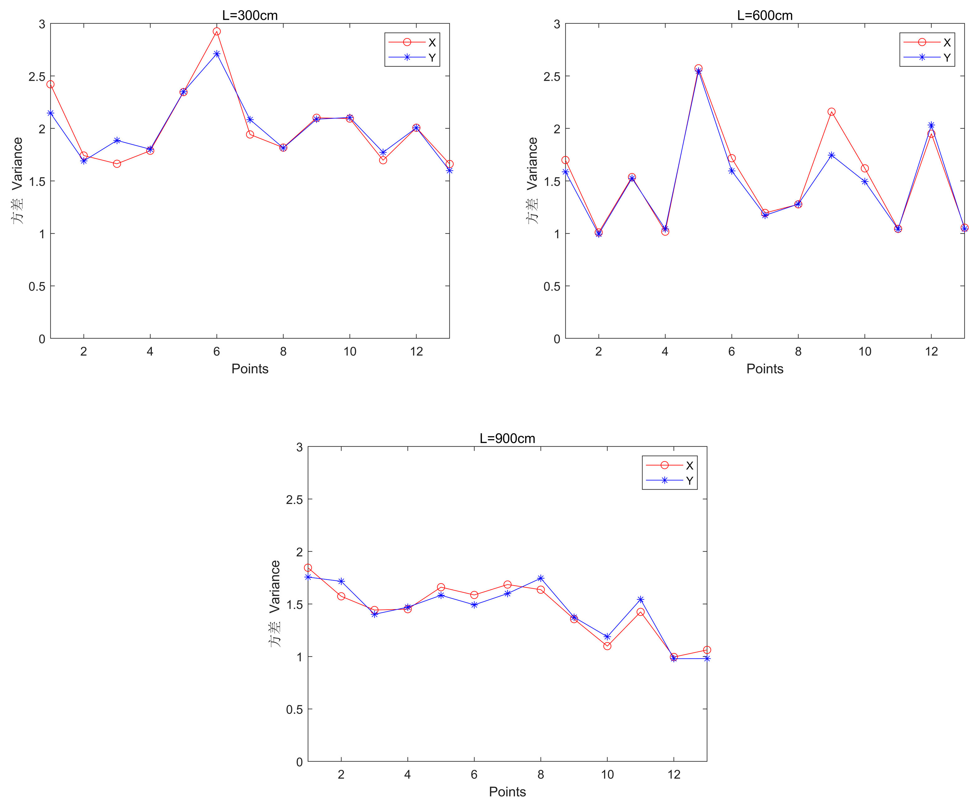
Comparison and analysis of the impact of different BTS spacing on positioning accuracy in the case of a BTS height of 175cm and a fixed square shape of BTS deployment, because the BTS fluctuates a lot when the BTS is deployed closer to each other, it is not possible to calibrate the BTS, so the spacing of the BTS deployment are: 300, 600, 900 squares, respectively.
Figure 13,
Figure 14 and
Figure 15 can be obtained: the root mean square error of each point of the three spacing cases, there is not much difference. when L=600 and 900, the variance of each point is smaller, basically within 1.5; while when L=300, the variance of each point is above 1.5.
Table 9 can be obtained that: when L=600, the maximum value of X is the smallest, when L=900, the minimum value of X and the average value are the smallest; when L=300, the maximum value of Y is the smallest, when L=900, the minimum value of Y is the smallest, and when L=600, the average value of Y is the smallest.
Table 10 can be obtained: when L=900, X, Y maximum and minimum and average values are the smallest, with the same spacing, the X, Y variance value of the same point does not differ much; the larger the spacing, the smaller the variance, that is, the more stable the positioning.
Different Shape of BTS arrangements
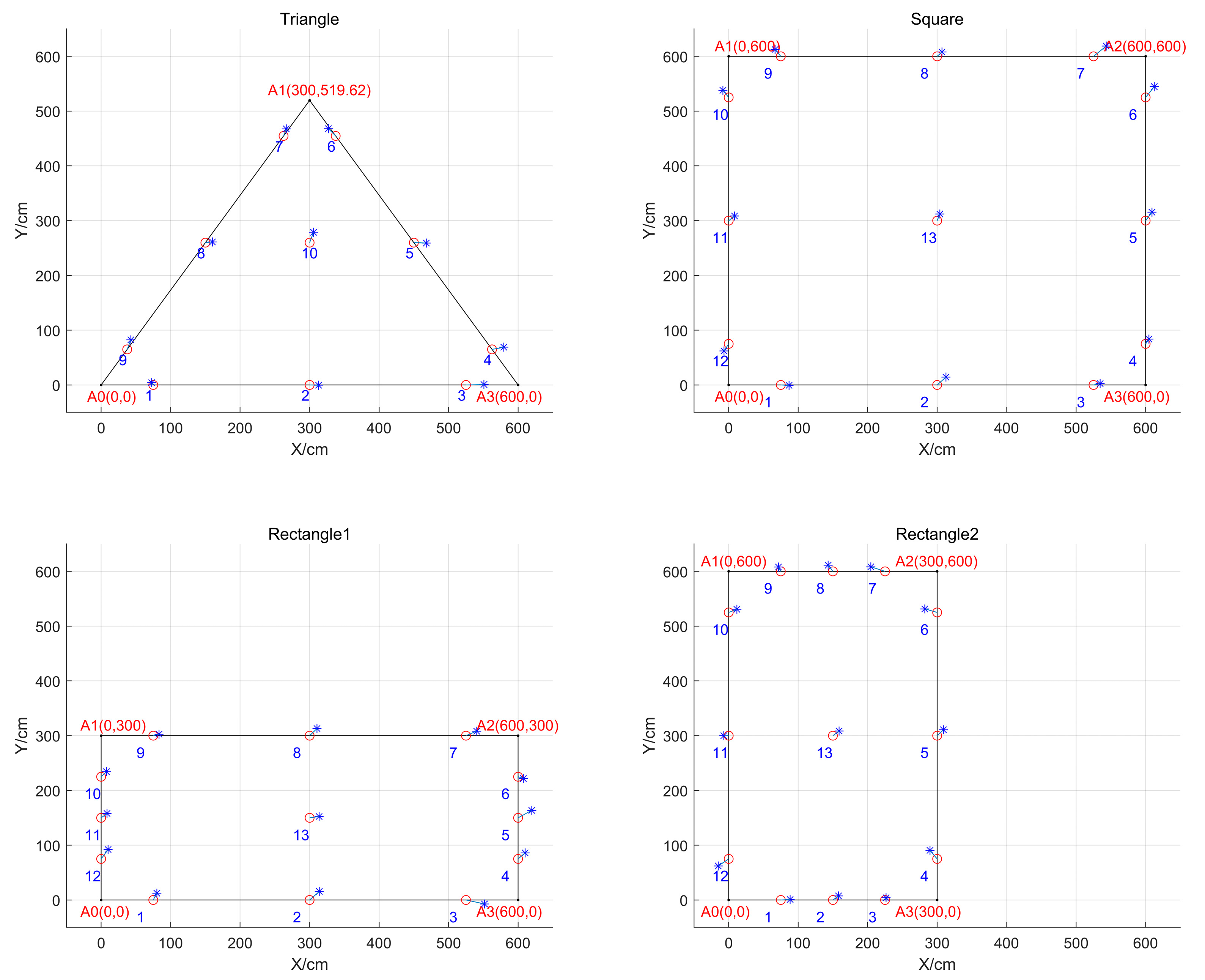
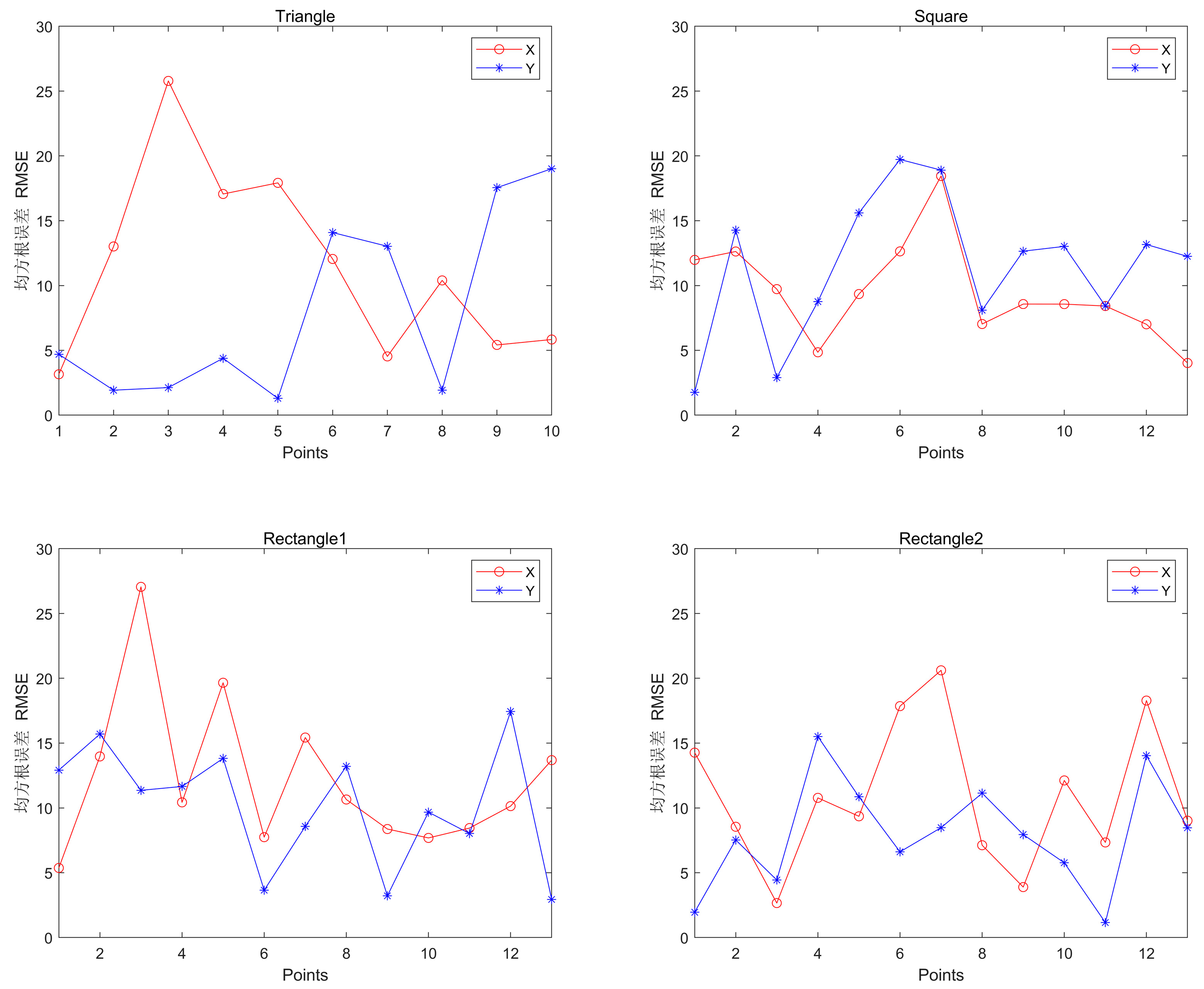
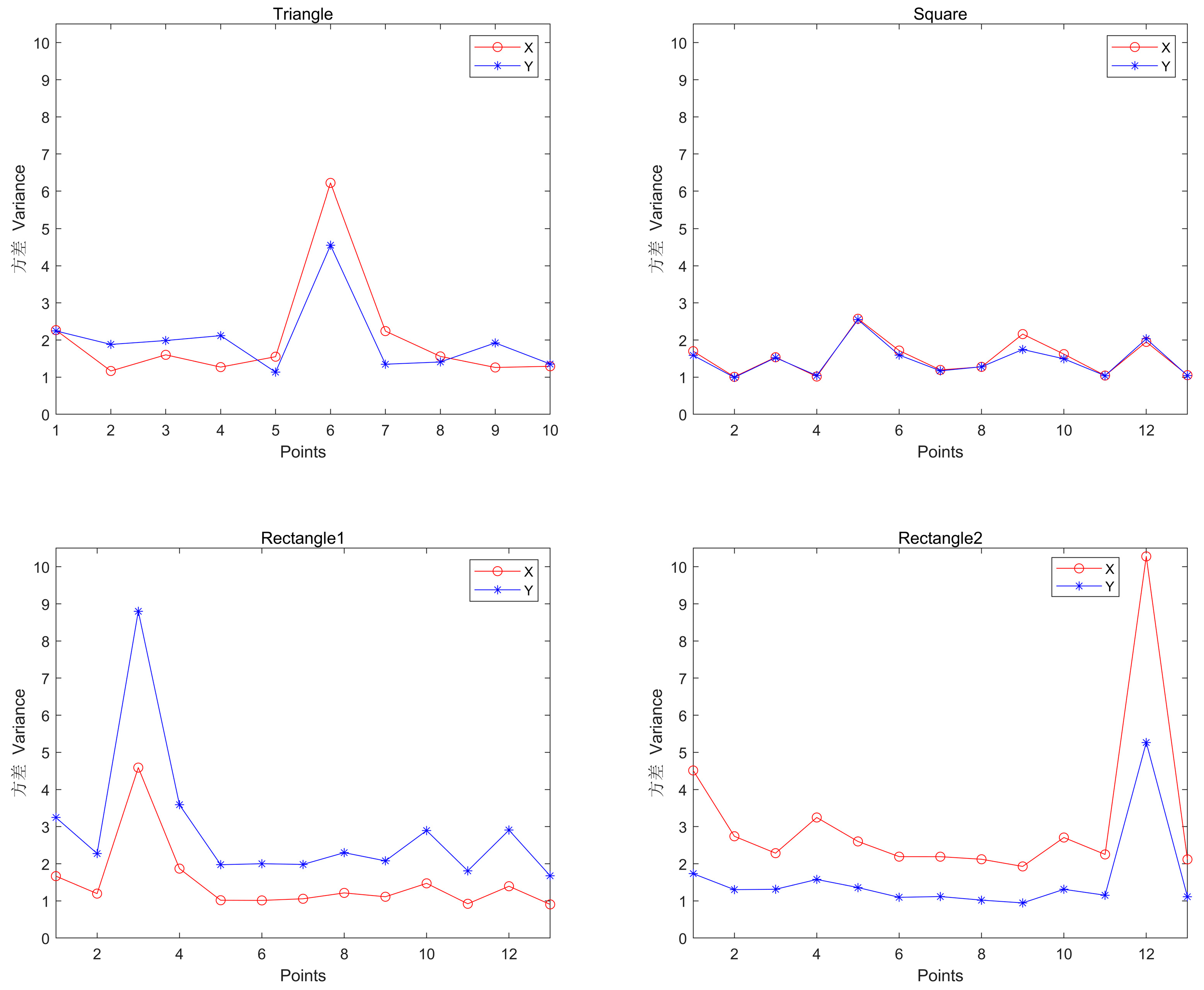
Comparison and analysis of the effect of different shapes of BTS layout on positioning accuracy in the case of fixed BTS spacing and BTS height, the BTS layout is set up as an equilateral triangle with a side length of 600cm, a square with a side length of 600cm, a rectangle with a length of 600cm and a width of 300cm, and a rectangle with a length of 300cm and a width of 600cm, respectively.
Figure 16,
Figure 17 and
Figure 18 show that when the BTS is set up as a square, the root mean square error of most points is below 15, and the X and Y variances are close to each other and are small. When the station is set up as a triangle or a rectangle, the root mean square error and variance of individual points are very large; when the station is set up as a rectangle, when the rectangle is larger than the width, the X variance of the same point is smaller than the Y variance; when the width of the rectangle is larger than the length, the Y variance of the same point is smaller than the X variance.
Table 11 can be obtained: the X maximum, minimum and mean of rectangle 1 are all the largest, the X maximum and mean of the square are all the smallest, and the X minimum of rectangle 2 is the smallest; the maximum and mean of Y of the square are all the largest, and the Y maximum, minimum and mean of rectangle 2 are all the smallest.
Table 12 shows that the maximum, minimum and mean values of X and Y are minimum for square X, maximum, minimum and mean values of X are maximum for rectangle 2 and maximum, minimum and mean values of Y are minimum for rectangle 1.
3.2.2. Dynamic positioning analysis
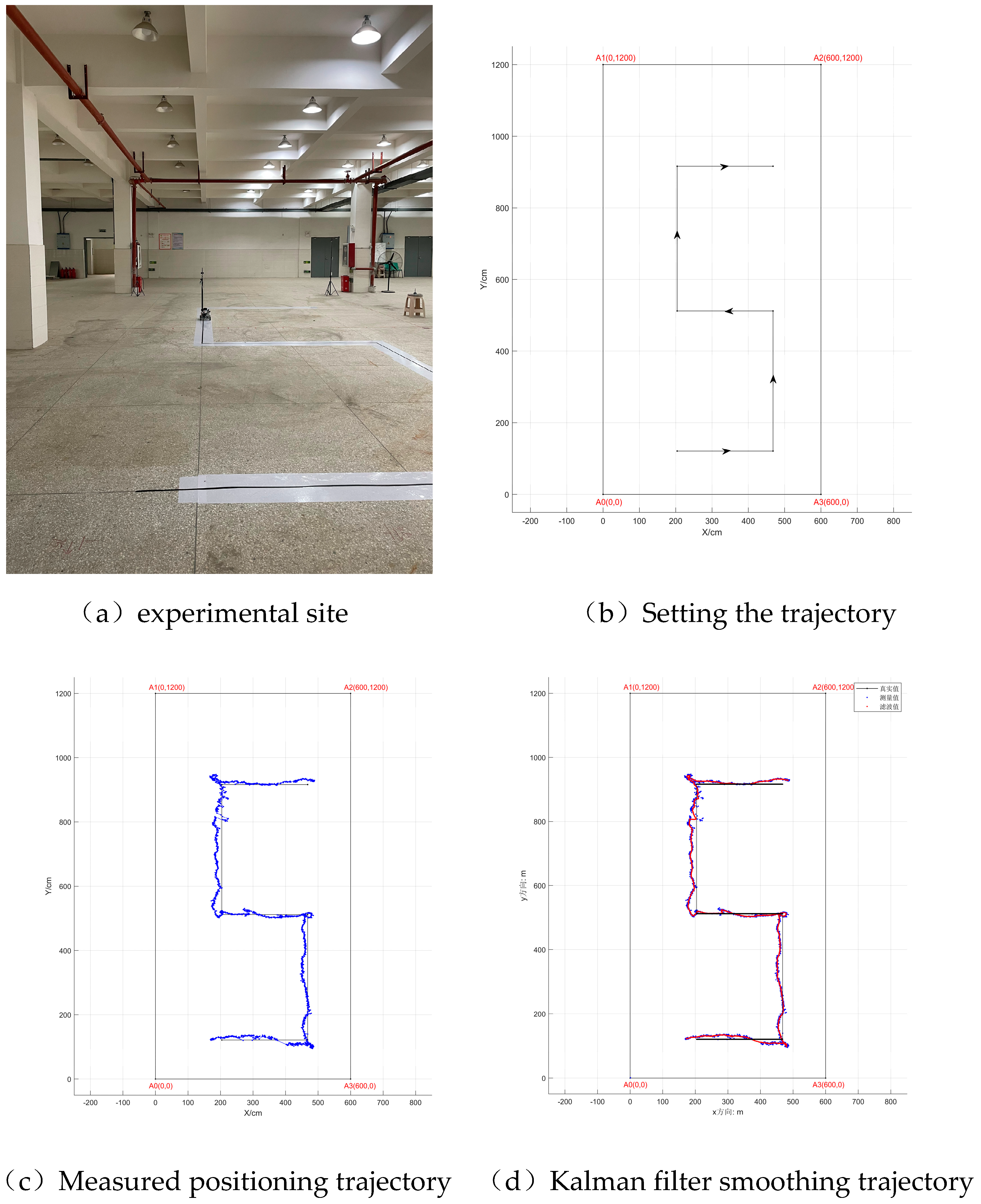
Dynamic experimental site selection in the 6m × 12m open hall in accordance with the established path, four UWB modules as a BTS height fixed at 175cm, a UWB module with a bracket rod fixed to the machine trolley, so that the positioning module is fixed at 1m from the ground, with a remote control to operate the trolley in accordance with the set path to dynamic positioning test, positioning system to 10HZ as the frequency, in the UWB positioning supporting the host PC software NAssistant, the positioning data is recorded and saved, experimental test track scene and equipment as shown in
Figure 19.
As can be seen from
Figure 19, when the trolley moves, the vertical coordinate offset in UWB following positioning is not large and the horizontal coordinate offset is large, and the positioning effect is better when the positioning trajectory moves horizontally than vertically.The UWB positioning is discrete points, and the use of Kalman filtering can be used to curve-smoothing and correcting the discrete positioning points.
4. Conclusion
For the UWB positioning effect in different deployment environments, based on the Matlab simulation positioning experiments and UWB measurement experiments, the effects of the height of the BTS deployment, the distance between BTS and the shape of the BTS deployment on the UWB positioning effect are investigated, the effects of the BTS deployment on the DOP value and the positioning error are simulated and analysed, and the static measurement experiments analyse the effects of the BTS deployment on the positioning effect of each point location, as well as the variance and the root-mean-square error, and the following conclusions are drawn:
(1) In the simulation experiment: in the closed area surrounded by the BTS, the closer to the centre, the smaller the HDOP value, the closer to the BTS, the smaller the VDOP and PDOP value, and the VDOP and PDOP values in the closed area are smaller than the average; outside the closed area, the DOP value is larger, and the further out the DOP value is larger. The suitable height of the BTS is 175~275, and the spacing of the BTS is better than 300cm for positioning effect, the BTS is laid out as a square positioning to give the best effect, and the positioning effect of the long side is better than the short side in the case of a rectangle.
(2) In the real experiment: when the BTS is set up as a square with a side length of 300cm, the height of the BTS can be adjusted to have an effect on the positioning effect, when the height of the BTS is 0 and 275, the positioning deviation is large and fluctuates greatly, and the appropriate height of the BTS should be 175-225cm.
(3) When the BTS is set up as a square with a height of 175cm, it can have an effect on the positioning effect by adjusting the BTS spacing. The smaller the BTS spacing, there will be individual points of root mean square error is very large; when the BTS spacing is less than 300cm, there will be the BTS itself calibration deviation of more than 100cm, calibration failure, can not be accurately positioning; spacing is greater than or equal to 300cm, UWB accuracy range, the larger the spacing, the more stable positioning.
(4) When the BTS is deployed as a triangle, square and rectangle with a height of 175 cm and a spacing of 600 cm, the variance of the X and Y coordinates of the square is similar and smaller, i.e., the positioning is the most stable, while the triangle and the rectangle will have a large deviation of individual points. When deployed as a rectangle, the long side is better than the short side for positioning.
(5) The deviation of the midpoint within the closed graph of the BTS deployment is the smallest, and the positioning effect is better.
(6) When the UWB performs following positioning, it will form discrete coordinate points in the host computer software, and the Kalman filter can be used to optimise the curve of the points.
(7) The results of the two experiments show that the positioning accuracy can be improved and the positioning effect optimised by adjusting the height of BTS deployment, the spacing between BTS and the shape of BTS deployment.
In the actual application scenario, the BTS deployment is limited by the environment and inevitably affected by multiple factors such as multipath effect, non-line-of-sight propagation, and multiple-site interference, which will cause large deviation in positioning, so the next experiment needs to study the effect of each interference object in the farm on the positioning effect on the basis of the specific deployment, and to establish the low-impact deployment model, so as to improve the positioning accuracy of the farm.
References
- Qian Minghui, Pan Fei, Qi Yu, POST-PANDEMIC DIGITAL ECONOMIC DEVELOPMENTS IN CHINA'S RURAL AREAS[J]. Chinese Journal of Agricultural Resources and Regional Planning,2021,42(11):62-71.
- Li Wei, Dong Guozhong, Zhou Yan. A look at the future of robotics in swine production[J]. Chinese Journal of Animal Science,2022,58(06):270-273.
- Li Dan, Chen Yifei, Li Xingjian, et al. Research Advance on Computer Vision in Behavioral Analysis of Pigs[J]. Journal of Agricultural Science and Technology,2019,21(07):59-69.
- Liu Feng, Wu Wenjie, Liu Xiaolei, et al. Progress of computer vision and deep learning methods for pig's identity and behavior recognition[J]. Journal of Huazhong Agricultural University, 2023,42(03):47-56.
- Xie Lei. Design and development of pig feed formulation system based on internet of things technology[J]. Feed Research,2021,44(17):104-108.
- Wang Ziquan, Yang Kefan, Li Leilei, et al. EFFECT OF ANIMAL DISEASE RISK ON APPLICATION OFDIGITALINTELLIGENCE TECHNOLOGY IN LARGE-SCALE PIG FARMS[J].Chinese Journal of Agricultural Resources and Regional Planning,2023,44(04):65-72.
- Zhao Rongyong, Zhang Haolin, Quan Wei, et al. UWB Positioning Technology and Intelligent Manufacturing Applications[M]. Beijing:CHINA MACHINE PRESS, 2020.01.
- Langley R B. Dilution of precision[J]. GPS world, 1999, 10(5): 52-59.
- Yu Mei. Research and Simulation on the Ultra Wide Band Wireless Positioning Algorithms[D]. Ocean University of China,2013.
- Langley R B. Dilution of precision[J]. GPS world, 1999, 10(5): 52-59.
- Li B, Dempster A G, Wang J. 3D DOPs for positioning applications using range measurements[J]. Wireless sensor network, 2011, 3(10): 334.
- Sharp I, Yu K, Guo Y J. GDOP analysis for positioning system design[J]. IEEE Transactions on Vehicular Technology, 2009, 58(7): 3371-3382.
- Guo Y, Li W, Yang G, et al. Combining Dilution of Precision and Kalman Filtering for UWB Positioning in a Narrow Space[J]. Remote Sensing, 2022, 14(21): 5409.
- Albaidhani A, Alsudani A. Anchor selection by geometric dilution of precision for an indoor positioning system using ultra-wide band technology[J]. IET Wireless Sensor Systems, 2021, 11(1): 22-31.
- 宋Song Qian, Zhang Bo, Li Shujian. Study of Configuration Technology of Ground Pseudolite [J].Computer Measurement & Control, 2013,21(03):743-746.
- LIU Chao, GAO Jingxiang, YU Ziyan, et al. An optimal pseudolites location model of GPS/pseudolites integrated relative positioning [J]. Journal of China University of Mining & Technology,2012,41(01):120-126.
- LI Haobo, WANG Jian, WANG Chuanyang. Discussion on affection factors of UWB indoor kinematic positioning[J]. Journal of Navigation and Positioning, 2018,6(01):45-48.
- Wang chuanyang, Wang Jian. Study of base station layout of ultra wideband emergency positioning[J]. Science of Surveying and Mapping,2019,44(08):174-181.
- Feng G, Shen C, Long C, et al. GDOP index in UWB indoor location system experiment[C]//2015 IEEE SENSORS. IEEE, 2015: 1-4.
- Yarlagadda R, Ali I, Al-Dhahir N, et al. Gps gdop metric[J]. IEE Proceedings: Radar, Sonar and Navigation, 2000, 147(5): 259-264.
Figure 1.
Contour plot of HDOP.
Figure 1.
Contour plot of HDOP.
Figure 2.
Contour plot of VDOP.
Figure 2.
Contour plot of VDOP.
Figure 3.
Contour plot of PDOP.
Figure 3.
Contour plot of PDOP.
Figure 4.
Contour plot of HDOP.
Figure 4.
Contour plot of HDOP.
Figure 5.
Contour plot of VDOP.
Figure 5.
Contour plot of VDOP.
Figure 6.
Contour plot of PDOP.
Figure 6.
Contour plot of PDOP.
Figure 7.
Contour plot of HDOP.
Figure 7.
Contour plot of HDOP.
Figure 8.
Contour plot of VDOP.
Figure 8.
Contour plot of VDOP.
Figure 9.
Contour plot of PDOP.
Figure 9.
Contour plot of PDOP.
Figure 10.
Positioning effect when the height of the BTS is different.
Figure 10.
Positioning effect when the height of the BTS is different.
Figure 11.
Root-mean-square error at each point with different heights of the BTS.
Figure 11.
Root-mean-square error at each point with different heights of the BTS.
Figure 12.
Variance plots for points with different heights of the BTS.
Figure 12.
Variance plots for points with different heights of the BTS.
Figure 13.
The effect of different spacing of BTS and simultaneous positioning.
Figure 13.
The effect of different spacing of BTS and simultaneous positioning.
Figure 14.
Root-mean-square error at each point when BTS spacing is different.
Figure 14.
Root-mean-square error at each point when BTS spacing is different.
Figure 15.
Variance at points with different BTS spacing.
Figure 15.
Variance at points with different BTS spacing.
Figure 16.
The effect of different shapes of BTS deployment and positioning at the same time.
Figure 16.
The effect of different shapes of BTS deployment and positioning at the same time.
Figure 17.
RMSE at each point when the shape of the BTS deployment is different.
Figure 17.
RMSE at each point when the shape of the BTS deployment is different.
Figure 18.
Variance at points with different shapes of BTS deployment.
Figure 18.
Variance at points with different shapes of BTS deployment.
Figure 19.
Dynamic Positioning Experiment.
Figure 19.
Dynamic Positioning Experiment.
Table 2.
DOP values for simulation experiments with different heights of BTS.
Table 2.
DOP values for simulation experiments with different heights of BTS.
| DOP |
Targets |
a |
b |
c |
d |
e |
f |
| HDOP |
maximum |
1.55 |
1.47 |
1.47 |
1.51 |
1.60 |
1.72 |
| minimum |
1.11 |
1.01 |
1.01 |
1.06 |
1.16 |
1.30 |
| average |
1.33 |
1.24 |
1.24 |
1.29 |
1.38 |
1.51 |
| VDOP |
maximum |
1.62 |
5.58 |
5.58 |
2.02 |
1.49 |
1.35 |
| minimum |
0.94 |
1.00 |
1.00 |
0.97 |
0.91 |
0.79 |
| average |
1.28 |
3.29 |
3.29 |
1.49 |
1.20 |
1.07 |
| PDOP |
maximum |
2.25 |
5.71 |
5.71 |
2.41 |
2.18 |
2.19 |
| minimum |
1.55 |
1.58 |
1.58 |
1.57 |
1.52 |
1.52 |
| average |
1.90 |
3.64 |
3.64 |
1.99 |
1.85 |
1.85 |
Table 4.
DOP values for simulation experiments with different BTS spacing.
Table 4.
DOP values for simulation experiments with different BTS spacing.
| DOP |
Targets |
a |
b |
c |
d |
e |
f |
| HDOP |
maximum |
1.65 |
1.51 |
1.49 |
1.48 |
1.47 |
1.47 |
| minimum |
1.22 |
1.06 |
1.03 |
1.02 |
1.01 |
1.01 |
| average |
1.44 |
1.29 |
1.26 |
1.25 |
1.24 |
1.24 |
| VDOP |
maximum |
1.41 |
2.02 |
2.88 |
3.77 |
4.67 |
5.58 |
| minimum |
0.86 |
0.97 |
0.99 |
0.99 |
1.00 |
1.00 |
| average |
1.13 |
1.49 |
1.93 |
2.38 |
2.83 |
3.29 |
| PDOP |
maximum |
2.17 |
2.41 |
3.13 |
3.96 |
4.82 |
5.71 |
| minimum |
1.50 |
1.57 |
1.57 |
1.58 |
1.58 |
1.58 |
| average |
1.84 |
1.99 |
2.35 |
2.77 |
3.20 |
3.64 |
Table 6.
DOP values for simulation experiments with different shapes.
Table 6.
DOP values for simulation experiments with different shapes.
| DOP |
Targets |
a |
b |
c |
d |
| HDOP |
maximum |
2.50 |
1.48 |
2.13 |
2.13 |
| minimum |
1.18 |
1.02 |
1.06 |
1.06 |
| average |
1.84 |
1.25 |
1.59 |
1.59 |
| VDOP |
maximum |
14.47 |
3.77 |
8.47 |
8.47 |
| minimum |
0.99 |
0.99 |
0.98 |
0.98 |
| average |
7.73 |
2.38 |
4.73 |
4.73 |
| PDOP |
maximum |
14.69 |
3.96 |
8.69 |
8.69 |
| minimum |
1.90 |
1.58 |
1.58 |
1.58 |
| average |
8.30 |
2.77 |
5.13 |
5.13 |
Table 7.
Root-mean-square error at each point with different heights of the BTS.
Table 7.
Root-mean-square error at each point with different heights of the BTS.
| X/Y |
Root Mean Square Error (RMSE) indicator |
H=0cm |
H=75cm |
H=125cm |
H=175cm |
H=225cm |
H=275cm |
| X |
maximum |
20.85 |
18.22 |
23.76 |
26.43 |
19.44 |
35.90 |
| minimum |
4.93 |
1.98 |
1.28 |
2.10 |
3.17 |
4.16 |
| average |
12.89 |
10.10 |
12.52 |
14.27 |
11.31 |
20.03 |
| Y |
maximum |
20.68 |
21.58 |
17.20 |
18.62 |
15.87 |
39.59 |
| minimum |
3.11 |
3.13 |
2.16 |
2.94 |
2.39 |
3.02 |
| average |
11.89 |
12.35 |
9.68 |
10.78 |
9.13 |
21.30 |
Table 8.
Variance at points with different heights of the BTS.
Table 8.
Variance at points with different heights of the BTS.
| X/Y |
variance indicator |
H=0cm |
H=75cm |
H=125cm |
H=175cm |
H=225cm |
H=275cm |
| X |
maximum |
2.29 |
3.69 |
2.73 |
2.92 |
3.12 |
6.12 |
| minimum |
1.55 |
1.34 |
1.23 |
1.66 |
1.39 |
1.63 |
| average |
1.92 |
2.51 |
1.98 |
2.29 |
2.26 |
3.88 |
| Y |
maximum |
2.29 |
4.02 |
3.05 |
2.71 |
3.08 |
6.04 |
| minimum |
1.58 |
1.41 |
1.28 |
1.60 |
1.41 |
1.54 |
| average |
1.94 |
2.72 |
2.17 |
2.15 |
2.25 |
3.79 |
Table 9.
Root-mean-square error at each point when BTS spacing is different.
Table 9.
Root-mean-square error at each point when BTS spacing is different.
| X/Y |
Root Mean Square Error (RMSE) indicator |
L=300cm |
L=600cm |
L=900cm |
| X |
maximum |
26.43 |
18.45 |
19.59 |
| minimum |
2.10 |
4.02 |
1.65 |
| average |
14.27 |
11.24 |
10.62 |
| Y |
maximum |
18.62 |
19.72 |
21.82 |
| minimum |
2.94 |
1.76 |
1.58 |
| average |
10.78 |
10.74 |
11.70 |
Table 10.
Variance at points with different BTS spacing.
Table 10.
Variance at points with different BTS spacing.
| X/Y |
variance indicator |
L=300cm |
L=600cm |
L=900cm |
| X |
maximum |
2.92 |
2.57 |
1.85 |
| minimum |
1.66 |
1.01 |
1.00 |
| average |
2.29 |
1.79 |
1.42 |
| Y |
maximum |
2.71 |
2.55 |
1.76 |
| minimum |
1.60 |
0.99 |
0.98 |
| average |
2.15 |
1.77 |
1.37 |
Table 11.
RMSE at each point when the shape of the BTS deployment is different.
Table 11.
RMSE at each point when the shape of the BTS deployment is different.
| X/Y |
Root Mean Square Error (RMSE) indicator |
Side length 600 equilateral triangle |
Side length 600 square |
600 long by 300 wide rectangular |
300 long by 600 wide rectangular |
| X |
maximum |
25.78 |
18.45 |
27.05 |
20.62 |
| minimum |
3.15 |
4.02 |
5.37 |
2.66 |
| average |
14.47 |
11.24 |
16.21 |
11.64 |
| Y |
maximum |
19.01 |
19.72 |
17.44 |
15.51 |
| minimum |
1.30 |
1.76 |
2.94 |
1.16 |
| average |
10.15 |
10.74 |
10.19 |
8.33 |
Table 12.
Variance at points with different shapes of BTS deployment.
Table 12.
Variance at points with different shapes of BTS deployment.
| X/Y |
variance indicator |
Side length 600 equilateral triangle |
Side length 600 square |
600 long by 300 wide rectangular |
300 long by 600 wide rectangular |
| X |
maximum |
6.22 |
2.57 |
4.59 |
10.28 |
| minimum |
1.17 |
1.01 |
0.91 |
1.93 |
| average |
3.69 |
1.79 |
2.75 |
6.10 |
| Y |
maximum |
4.55 |
2.55 |
8.80 |
5.27 |
| minimum |
1.14 |
0.99 |
1.68 |
0.95 |
| average |
2.84 |
1.77 |
5.24 |
3.11 |
|
Disclaimer/Publisher’s Note: The statements, opinions and data contained in all publications are solely those of the individual author(s) and contributor(s) and not of MDPI and/or the editor(s). MDPI and/or the editor(s) disclaim responsibility for any injury to people or property resulting from any ideas, methods, instructions or products referred to in the content. |
© 2023 by the authors. Licensee MDPI, Basel, Switzerland. This article is an open access article distributed under the terms and conditions of the Creative Commons Attribution (CC BY) license (http://creativecommons.org/licenses/by/4.0/).
