Generalized SmartScan: An Intelligent LPBF Scan Sequence Optimization Approach for 3D Part Geometries

1. Introduction

Laser powder bed fusion (LPBF) is a prominent technique within the field of additive manufacturing (AM) of metals that is finding applications across diverse industries, including aerospace, automotive, and biomedical. This method employs high-intensity lasers to systematically melt powder, layer by layer, resulting in the creation of intricate 3D objects. Compared to other metal AM techniques, LPBF excels in fabricating complex parts with high precision at relatively high build speeds as indicated by Yang et al., (2023) and Sames et al., (2016). Nevertheless, LPBF-produced parts are susceptible to residual stress, deformation, and related defects stemming from non-uniform thermal distribution as highlighted by Parry et al., (2016) and Dong et al., (2022). While post-process heat treatments can ameliorate some of these issues, they are often time-consuming, costly (Chen et al., 2021), and insufficient in rectifying deformation or cracks induced by thermal stresses during the build process (Cao et al., 2021; Guo et al., 2020; Khan et al., 2021). Consequently, it is critical to minimize temperature gradients during the build process to assure quality (Kumar & Jebaraj, 2023).

Numerous studies have highlighted the critical role of scanning strategy in achieving uniform temperature distribution and defect-free printing via LPBF. The umbrella term “scan strategy” encompasses a variety of approaches for altering scanning parameters, such as beam power, scan speed, hatch spacing, scan pattern, and layer thickness. For instance, Reiff et al., (2021), Cao et al., (2023), Riensche et al., (2022), and Wang et al., (2023) have investigated altering laser power or speed, while Boissier et al., (2022), Kim & Hart, (2022), Liu et al., (2022), and Qin et al., (2023) have explored scanning path optimization with the aim of minimizing thermal gradients and distortion in LPBF. Kaleli Alay et al., (2023) introduced a scanning method, termed time-homogenization (TH), to manage the morphology of the brittle Laves phase in LPBF of Inconel 718, thus enhancing the material’s mechanical properties at both room and elevated temperatures when compared to samples built using standard scanning strategies.

Scan sequence, which is another integral component of scan strategy, has garnered increasing attention as a means to reduce thermal gradients and enhance print quality in LPBF. Scan sequence pertains to the order in which a predetermined geometric scan pattern is traced. For instance, two of the most commonly employed scan patterns are the stripe and island patterns, as investigated by the authors Ramani et al., (2022) and He et al., (2023) in a prior study. The sequence within these patterns can refer to the order in which each line in the stripe pattern is scanned or the order in which each island in the island pattern is scanned. Research has shown that scan sequence significantly impacts temperature distribution, residual stress, and distortion in LPBF. Consequently, various methods have been proposed to determine scan sequences that minimize thermal gradients, residual stress, and distortion. For example, Kruth et al., (2004) proposed LHI, least heat influence, involving the scanning of sectors in a specific order, beginning with a randomly selected sector and then scanning the sector that is least heated (farthest away from the preceding sector). A similar approach to LHI was adopted by Qin et al., (2023) who proposed a scan sequence algorithm for island-based strategy which chose the island with the maximum distance from the currently active island until all islands had been traversed. Mugwagwa et al., (2019) evaluated four scan sequences, namely, island, successive, successive chessboard, and LHI, in terms of their impact on residual stress and distortion, demonstrating that the choice of scan sequence resulted in the reduction of maximum distortion and up to 40% reduction in residual stress. Pant et al., (2022) proposed sectional strategies that divided layers into three separate sections and scanned either the outermost section or the innermost section first for each layer. However, parts printed using their strategy exhibited a high incidence of cracks and porosity at the interface between the sections. Ramos et al., (2019) proposed an intermittent scan sequence for the island scan pattern. Their method avoids scanning adjacent islands consecutively by using a geometry-based formula having weights and radial thresholds. Using their strategy, they demonstrated a 10% reduction in deformation compared to an alternating scan sequence, for the same vector length.

As noted in earlier work (Ramani et al., 2022), a deficiency shared by the existing methods for scan sequence generation is that they are highly dependent on heuristic formulations that approximate heat transfer in LPBF using geometric relationships that do not generalize well. To address this shortcoming, Ramani et al., (2022) introduced SmartScan, an intelligent scan sequence generation approach for LPBF. SmartScan differentiates itself from heuristic techniques by utilizing thermal models of LPBF combined with rigorous control-based optimization techniques to determine optimal scan sequences, ensuring its generalizability. The application of SmartScan to laser marking of AISI 316 L stainless steel plates in (Ramani et al., 2022) demonstrated up to 41% and 47% reductions in thermal inhomogeneity and distortion, respectively, compared to state-of-the-art heuristic methods. Moreover, SmartScan exhibited notable robustness and computational efficiency, making it suitable for online implementation. Subsequent work has expanded SmartScan to encompass complex geometries (He, Ramani, et al., 2022) advanced scan patterns (He, Tsai, et al., 2022), and multi-laser PBF systems (He et al., 2023). However, these prior works were limited to 2D part geometries and lacked the capability to handle 3D parts with arbitrary scan patterns and geometric features, which are typical in LPBF. To address these limitations, building on preliminary work (He & Okwudire, 2023), this paper introduces a generalized SmartScan algorithm applicable to LPBF of arbitrary 3D parts. The paper makes the following original contributions to the literature (see Figure 1):

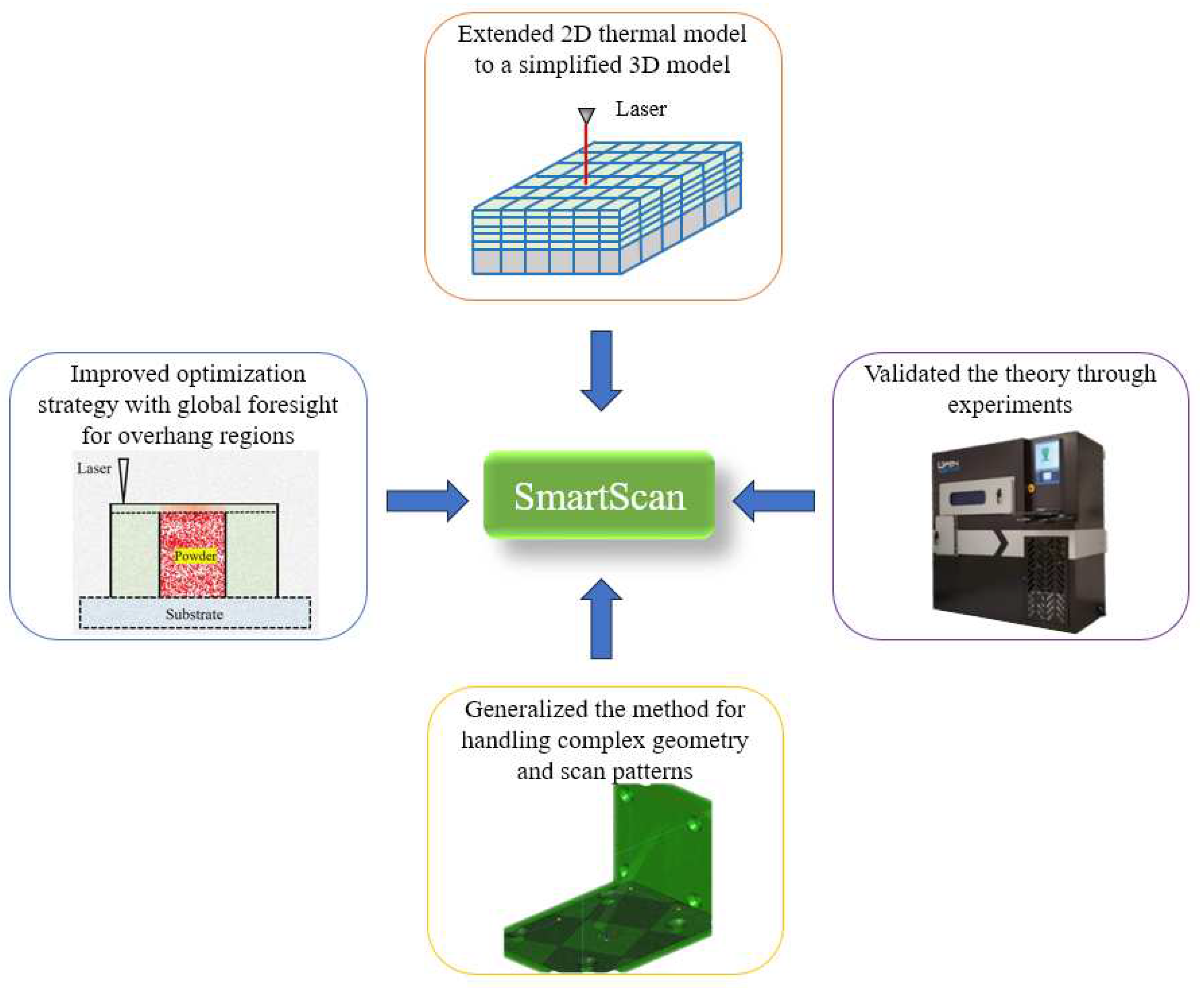
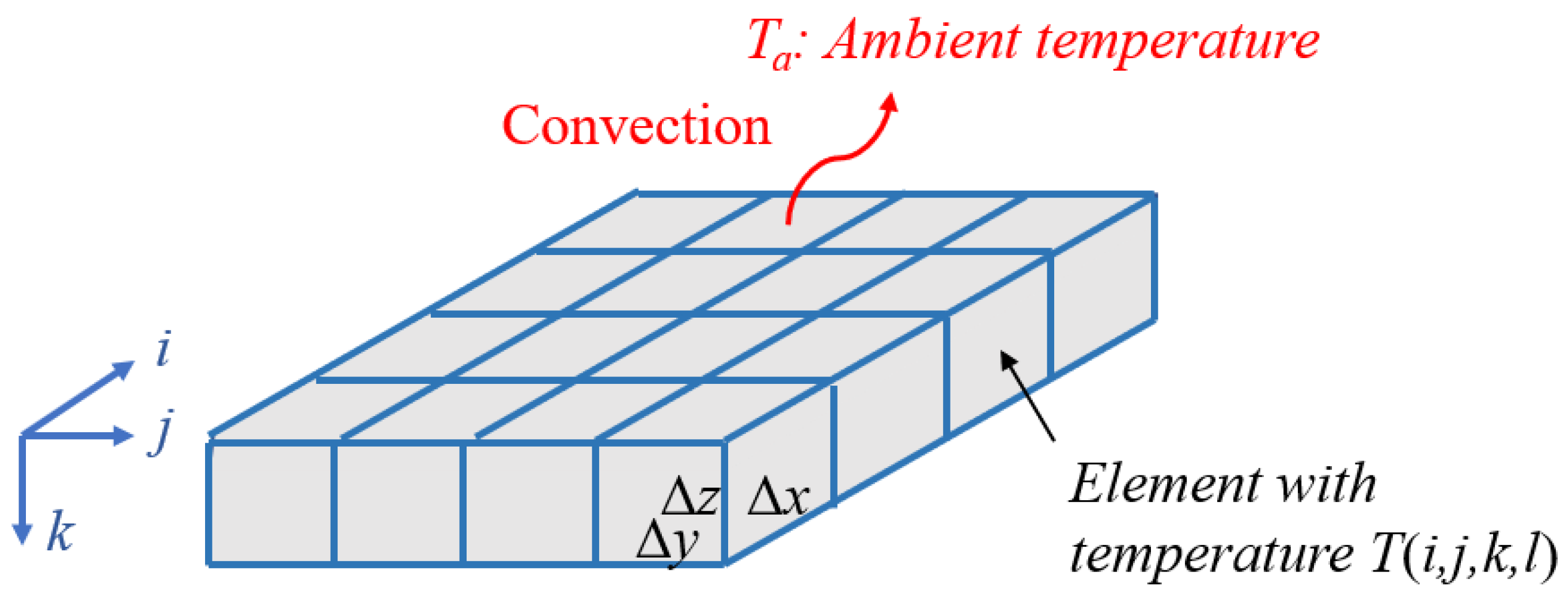
• It extends the 2D thermal model and objective function of the original SmartScan (Ramani et al., 2022) to incorporate 3D thermal effects, while introducing simplifying assumptions to reduce computational complexity due to larger model sizes.
• It generalizes the original SmartScan modeling and optimization methods to enable them to handle arbitrary scan patterns with scan vectors of varying lengths and inclination angles within each layer.
• It addresses the greedy (myopic) optimization strategy of prior versions of SmartScan by incorporating global foresight into the generalized SmartScan, enabling it to optimize temperature distribution more effectively in 3D parts with overhangs and other geometric features that can trap heat.
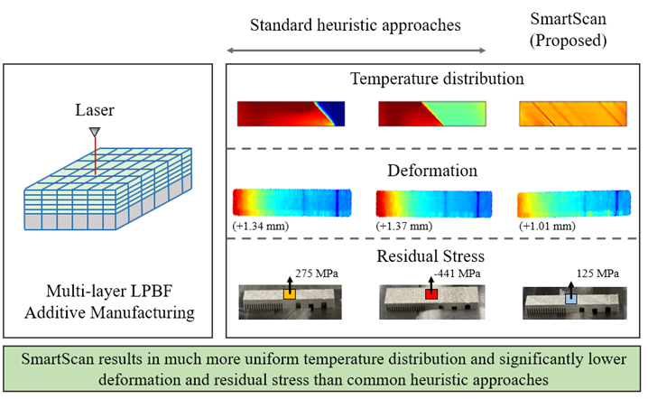
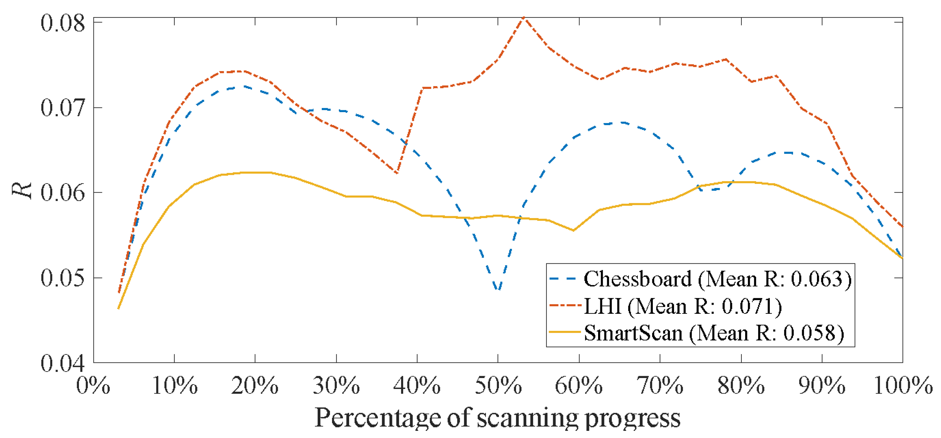
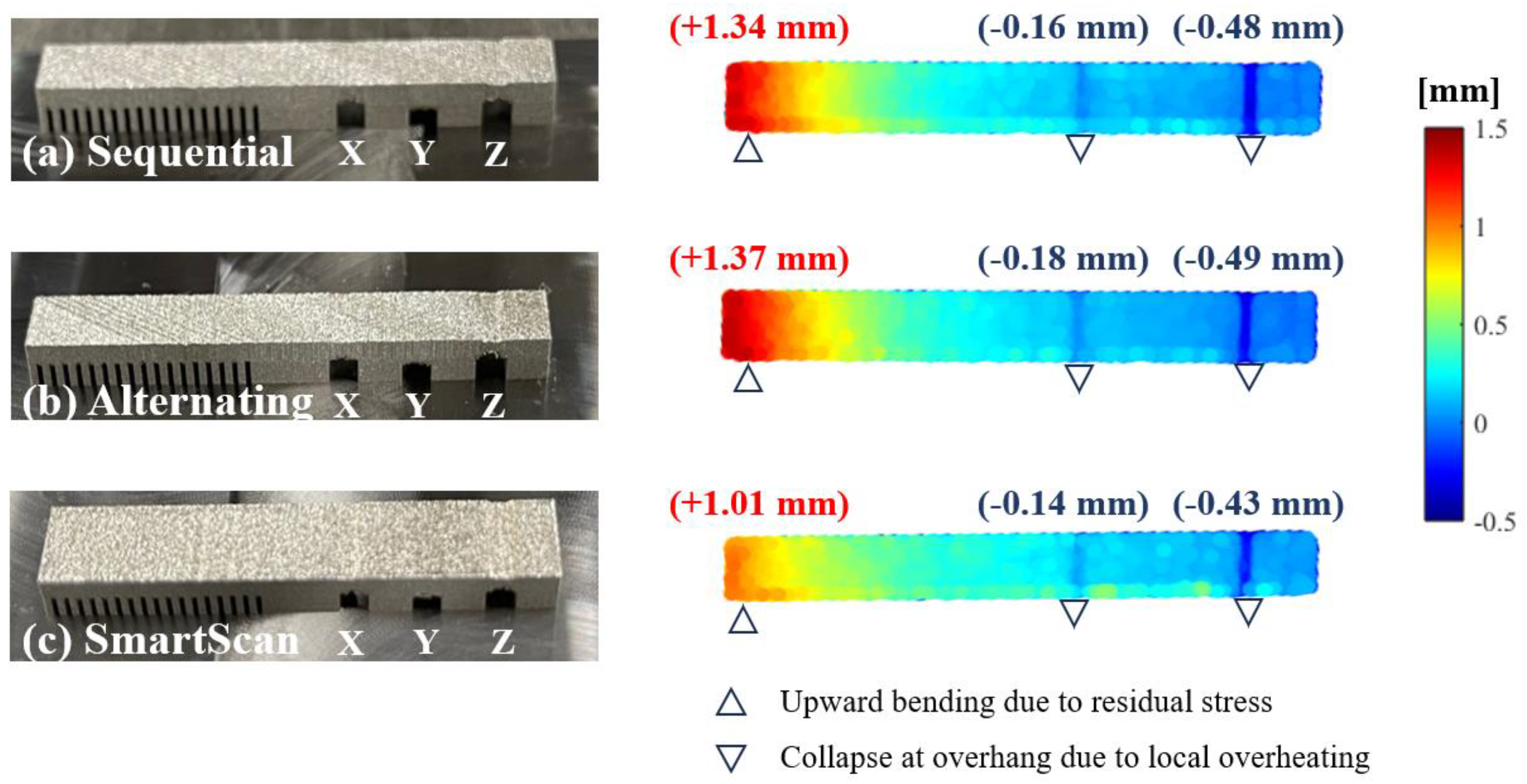
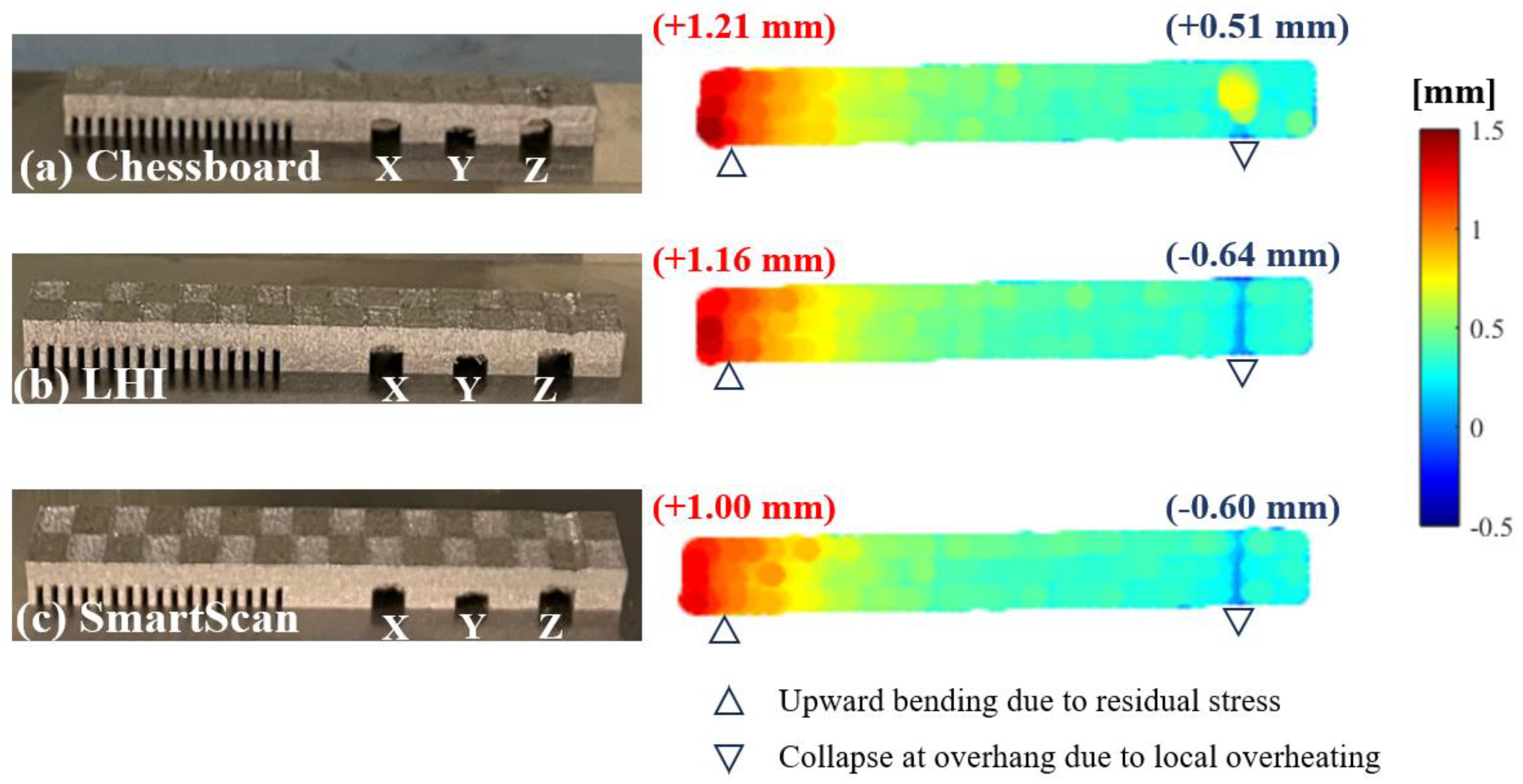
• It validates the effectiveness of the generalized SmartScan through simulations and experiments involving the printing of a complex 3D shape using AISI 316L stainless steel. The results demonstrate significantly reduced thermal inhomogeneity, residual stress, and distortion compared to standard heuristic scan sequences, at the expense of some increases in surface roughness.

The remainder of this paper is organized as follows: Section 2 offers a brief review of the original SmartScan model for single-layer systems, as detailed in (Ramani et al., 2022), and then broadens the scope of the SmartScan to multi-layer LPBF with arbitrary geometric features and scan patterns. Section 3 presents simulation case studies to compare SmartScan with current heuristic scanning approaches for both stripe and island cases. Section 4 demonstrates SmartScan’s effectiveness in minimizing thermal-induced distortion and residual stress, compared to state-of-the-art heuristic scan sequences. The paper concludes with Section 5, which summarizes the key findings and outlines avenues for future research.

2. Methodology

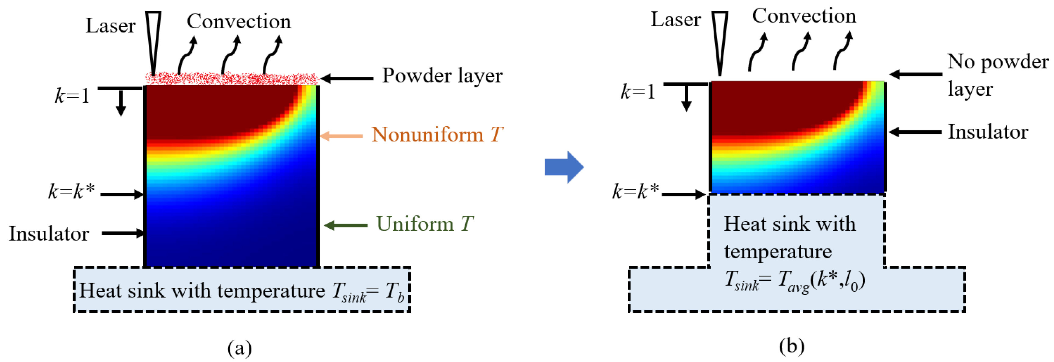
2.1. Extension of SmartScan Thermal Model and Optimization to Multiple Layers

This section provides an overview of SmartScan and how its underlying thermal model and optimization approach are generalized to handle 3D geometries with multiple layers. As in our prior work on SmartScan (Ramani et al., 2022), we adopt a model that considers only conductive and convective heat transfer between the part being printed and its surroundings (See Figure 2). Radiative heat transfer, latent heat effects, Marangoni convection, and other melt pool phenomena, are ignored. These assumptions are reasonable because SmartScan focuses on part-scale temperature distribution. The model parameters are assumed to be temperature-independent to keep the model linear, which is critical for efficient optimization. In our prior work (Ramani et al., 2022), we have demonstrated that this simplification does not significantly diminish the effectiveness of SmartScan. Accordingly, heat transfer within the printed part with conductivity k_t and diffusivity α can be described using the equation:

$$\frac{{\partial }^{2}T}{\partial x^2}+\frac{{\partial }^{2}T}{\partial y^2}+\frac{{\partial }^{2}T}{\partial z^2}+\frac{u}{k_t}=\frac{1}{\alpha }\frac{\partial T}{\partial t}$$

(1)

where T is the temperature, x, y and z are the spatial coordinates, t is time and u is the power per unit volume. The finite differences method (FDM) can be used to discretize Eq.(1) to obtain

$$\begin{array}{l}\frac{T\left(i+1,j,k,l\right)+T\left(i-1,j,k,l\right)-2T\left(i,j,k,l\right)}{\Delta x^2}\\ +\frac{T\left(i,j+1,k,l\right)+T\left(i,j-1,k,l\right)-2T\left(i,j,k,l\right)}{\Delta y^2}\\ +\frac{T\left(i,j,k+1,l\right)+T\left(i,j,k-1,l\right)-2T\left(i,j,k,l\right)}{\Delta z^2}\\ +\frac{u\left(i,j,k,l\right)}{k_t}=\frac{1}{\alpha }\frac{T\left(i,j,k,l+1\right)-T\left(i,j,k,l\right)}{\Delta t}\end{array}$$

(2)

where Δx, Δy and Δz are the dimensions of each element (see Figure 2), i, j and k are the spatial indices of the elements, l is the temporal index (i.e., t = lΔt), Δt is the time step and T(i,j,k,l) is the temperature of the element located at (i,j,k) at time l. Without loss of generality, the element height Δz is assumed to be equal to the layer height of the LPBF process, such that k serves as an index for deposited layers (referenced to the topmost layer where k = 1).

Two main factors must be considered in extending the 2D Smartscan model used in our prior work (Ramani et al., 2022) to 3D, namely: (1) a powder layer and (2) multiple printed layers underneath the powder layer. The powder can be considered as an insulator since its conductivity is roughly an order of magnitude lower than that of solid metal (Wei et al., 2018). However, during printing, the conductivity of the powder layer changes continuously as portions of it are converted from powder into solid metal. This means that some conductive heat transfer is bound to occur within the powder layer, resulting in a time-varying thermal model. However, the intra-layer heat conduction of the powder layer is negligible since the powder layer is very thin (typically 20 to 100 μm in thickness (Mahmoodkhani et al., 2019)). Hence, most of the heat transfer that affects temperature distribution occurs due to conduction into the layers below rather than within the powder layer.

Therefore, for the sake of simplicity, we neglect the powder layer in our model and apply the laser power directly to the layer beneath the powder, as depicted in Figure 3. Moreover, the substrate (base plate) is assumed to be a heat sink held at a constant uniform temperature T_b. The sides of the part are insulated by the low-conductivity powder and heat is lost by convection through the top layer. As layers are built during the printing process, the heat from the laser is conducted down into the substrate. Therefore, it can be expected that the heat distribution becomes reasonably uniform at some layer k = k* from the top surface. Since SmartScan is focused on maintaining uniform temperature distribution and not on modelling the absolute temperature, the model can be simplified by replacing the layers k > k* with a heat sink at a uniform temperature T_sink. One benefit of this approximation is that the model size can be reduced to only consider 1 ≤ k ≤ k*, as shown in Figure 3(b).

To determine k* and T_sink, the temperature uniformity metric R(k,l) presented in (Ramani et al., 2022) is used:

(3)

where T_avg(k,l) denotes the mean of the temperatures T(i,j,k,l) of a layer k at time l, s signifies the number of elements of the corresponding layer k, and T_m represents the melting point of the material used to normalize R. As layers are built, the value of R is computed at the beginning of each new layer (i.e., at time l = l₀) for all layers k ≥ 1. Accordingly, k* can be determined as the value of k for which R(k*, l₀)/R(1, l₀) < ε, where ε is a predetermined uniformity criterion (e.g., 5%) such that T_sink = T_avg(k*,l₀) can be used as the Dirichlet boundary condition at the bottom of the simplified model in Figure 3(b). Note that R(1, l₀) is used to normalize R(k*, l₀) because it typically represents the layer with the worst thermal uniformity, since it lies just below the powder layer. Also note that the value of k* cannot exceed the total number of layers in the part at any given time.

Based on the simplifications to the 3D thermal model discussed above, Eq. (2) can be rearranged into a state space equation

(4)

Here, T(l) refers to the state vector, encapsulating the thermal information T(i,j,k,l) for all elements in the region 1 ≤ k ≤ k* at time l. The state matrix is denoted by A, while B is the input matrix. The sparse vector u(l) denotes the power input; its non-zero elements coincide with the application location of the laser. The influence of heat transfer through convection to the ambient temperature T_a, with the convection coefficient h, and conduction to the layers below k* with a temperature of T_sink are incorporated into the model following the heat sink approach described in (Ning et al., 2019). Also, the laser beam’s heat flux is characterized by a Gaussian distribution (Ramos et al., 2019).

Assuming that it takes n_p time steps to scan each feature, as discussed in (Ramani et al., 2022), the corresponding representation of the state-space at the feature level with the time index, l_p, can then be expressed as follows

(5)

The objective of SmartScan is to minimize temperature inhomogeneity for each printed layer, which is achieved by minimizing the temperature uniformity metric R(1,l_p) of the topmost layer of our model (i.e., the layer just below the powder layer) which can be written as

(6)

where 1 represents a column vector of length s whose all elements are equal to 1, I is an identity matrix, and the 0 (null) matrix in the $\widehat{\mathbf{C}}$matrix indicates that the elements of T beyond the first layer, T_sink and the ambient temperature T_a do not contribute to the calculation of R. The optimization problem can therefore be expressed as

(7)

where  = A_p, the columns of B̂ represent the corresponding b vectors as in Eq. (5) for each feature, and û(l_p) is a vector with only one element equal to 1 and all other elements equal to 0. The location of 1 in û(l_p) represents the column of B̂ corresponding to the feature to be scanned.

The objective function expressed in Eq. (7) can be reformulated as follows:

(8)

Subsequently, the optimization problem for the topmost layer can be reformulated in the following manner:

(9)

where $\mathsf{\Gamma }\triangleq {\widehat{\mathbf{B}}}^{\mathrm{T}}{\widehat{\mathbf{C}}}^{\mathrm{T}}\widehat{\mathbf{C}}\widehat{\mathbf{B}}$ $\mathrm{a}\mathrm{n}\mathrm{d}\mathsf{\Lambda }\triangleq {\widehat{\mathbf{B}}}^{\mathrm{T}}{\widehat{\mathbf{C}}}^{\mathrm{T}}\widehat{\mathbf{C}}\widehat{\mathbf{A}}$, with n_f denoting the number of features in the topmost layer. Furthermore, the rth diagonal element of the Γ matrix is denoted as Γ(r,r), and the rth row of the Λ matrix is referred to as Λ(r,:).

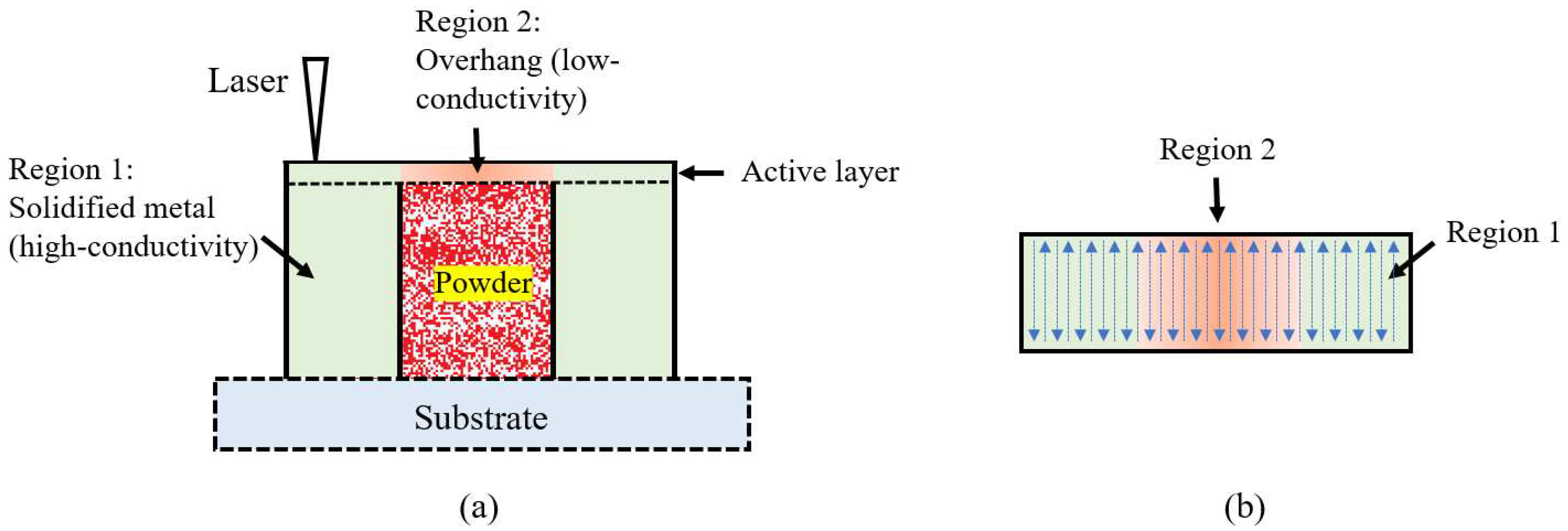
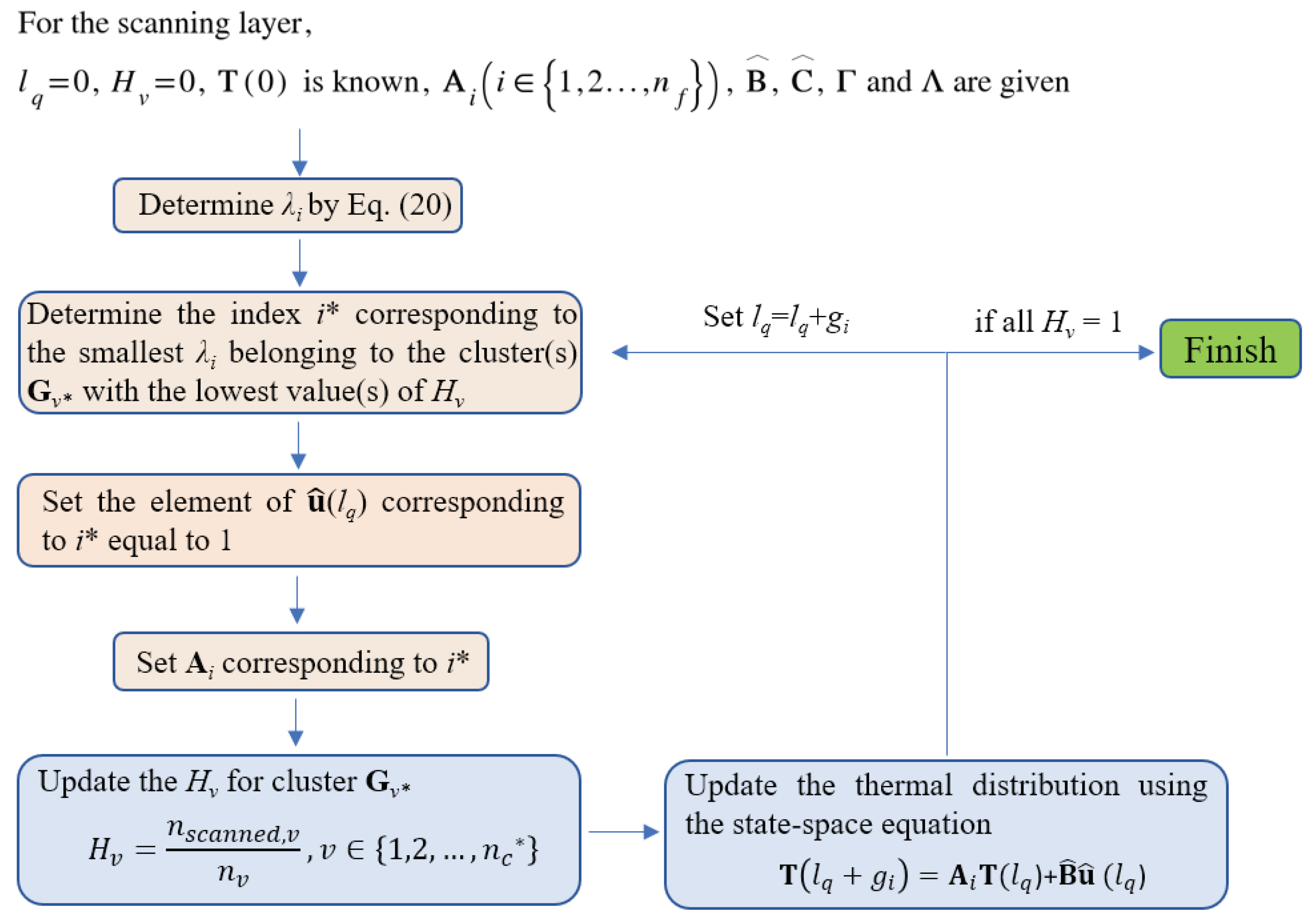
2.2. Providing SmartScan with Global Foresight

A critical problem with the SmartScan optimization algorithm, as described in Section 2.1 above (and in our prior work (He et al., 2023; Ramani et al., 2022)) is that it is myopic. It minimizes R(1,l_p) for any given feature without a global foresight of the impact of its current actions on future outcomes. This limits its effectiveness for complex 3D shapes. To illustrate the problem, consider a part with an overhang whose cross-section is shown in Figure 4(a). The part has a uniform depth into the page. At the print stage shown in the figure, the part can be divided into two regions – Region 1 supported by high-conductivity solid metal and Region 2 supported by low-conductivity powder. On the active layer of the print shown in Figure 4(b), Region 1 has two times the number of scan vectors as Region 2. In optimizing the sequence of the stripes in the active layer, the myopic SmartScan algorithm would prioritize scanning the stripes in Region 1 because they yield lower R(1,l_p) values by conducting heat quickly to the bottom layers. Therefore, at the end, the algorithm is left with most of the stripes from Region 2 to scan, leading to extremely inhomogeneous thermal distribution and overheating of Region 2 toward the end of the scanning process.

In this Section, we address this limitation of SmartScan by providing it with global foresight of the heat transfer of the layer whose scan sequence it is optimizing. At a high level, our solution consists of two steps. Firstly, we demarcate the features into clusters based on their relative heat transfer behavior (e.g., features in Region 1 and Region 2 in Figure 4). Secondly, we constrain the SmartScan optimization so that no cluster is left behind in the scanning. In the context of the simple example in Figure 4(b), this means that for every two stripes scanned in Region 1, one stripe must be scanned in Region 2. These two steps are detailed and generalized below.

2.2.1. Demarcation of the Features into Clusters based on Heat Transfer

The challenge addressed here is how to demarcate the features of any arbitrary geometry into clusters based on heat transfer. We make use of the fact that the diagonal elements of the matrix  in Eq. (7) contain information about the relative heat transfer characteristics of each element of our FDM model because their magnitude is inversely proportional to the element’s rate of heat dissipation to the surrounding elements. Therefore, we extract the diagonal elements of  as:

(10)

where sa represents the number of elements in the active layer where k=1. Then we apply the K-means method (Ahmed et al., 2020) to D (which represents the dataset) as follows:

• Divide the dataset into n_c clusters G_v, where v = 1, 2, …, n_c, by iteratively assigning each data point d_i to the cluster with the nearest centroid and then updating the centroid of each cluster until convergence is achieved.
• Compute the sum of squared errors (SSE) for increasing values of n_c, starting from n_c = 1, using the formula given by

  

  (11)

  where m_v refers to the centroid (mean) of the cluster G_v.
• Determine the optimal number of clusters (n_c*) using the “elbow method” (F. Liu & Deng, 2021) which indicates the value of n_c at which the SSE vs. n_c graph exhibits an inflection. Approximate the elbow point by calculating the second derivative of the SSE vs. n_c curve, and choose the point where the second derivative is highest (i.e., where the rate of change of the gradient is highest) as

  

  (12)

  where SSE’’(n_c) represents the second derivative of the SSE as a function of n_c.
• Using n_c*, determine the optimal clustering of the dataset D. The number of clusters represents the number of regions in a layer based on heat transfer.
• The clustering described in Step 4 is at the finite difference method (FDM) element level. The features are assigned to the n_c* clusters based on the cluster v to which most of their elements belong. For example, if 100 elements in a feature belong to G₁ and 20 elements belong to G₂, then the feature will be assigned to G₁.

2.2.2. Proportional Scanning of Features in Every Cluster with Global Foresight

One way of providing global foresight to the SmartScan optimization algorithm is to force it to scan each cluster in proportion to the number of features it contains. In other words, it ensures that no cluster is left behind as it optimizes the sequences. To do this, we define n_v as the number of features in cluster G_v, as well as a completion index H_v = n_scanned,v/n_v, where n_scanned,v represents the number of features scanned in cluster G_v at any given time.

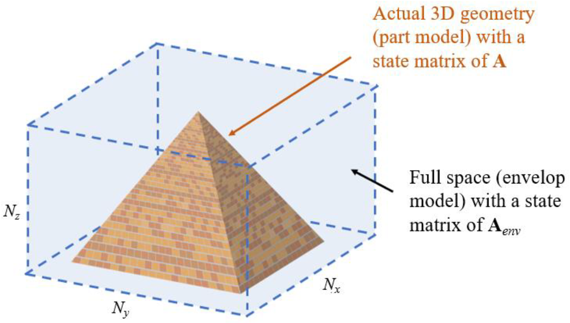
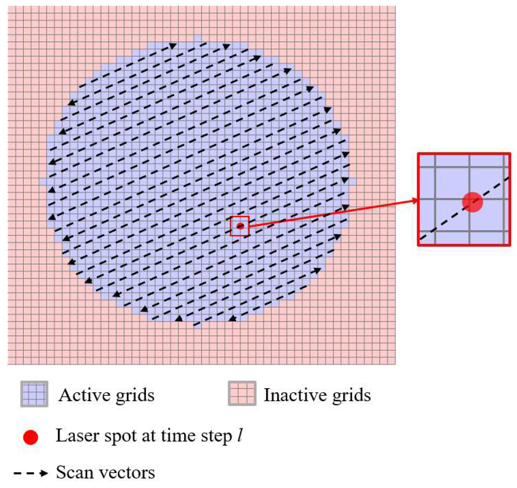
2.3. Incorporation of Ability to Handle Arbitrary Part Geometries and Scan Patterns

The SmartScan algorithm discussed so far cannot handle arbitrary part geometries and scan patterns because of the following assumptions that have been made in our prior work (Ramani et al., 2022): (1) the FDM model is customized for the geometry and scan pattern of each layer (e.g., the scan vectors always align with the x or y directions of the FDM model with a hatch spacing that is equal to the grid spacing of the FDM model); and (2) all features have the same size and are scanned at the same speed such that they take an equal number of time steps n_p to be scanned as described in Eq. (5). In this section, we relax these assumptions, allowing SmartScan to apply to arbitrary part geometries and scan patterns.

To relax the first assumption, the FDM model is decoupled from the geometric shape of the 3D part to be optimized by designing the FDM grid to envelop the entire part as shown in Figure 5 using a pyramid as an example. This allows arbitrary shapes to be captured by the envelop model of size n_env = N_x x N_yx N_z elements as shown in Figure 5. Accordingly, the state space equation representing the envelop model can be written as

(13)

where T_env, A_env, B_env and u_env retain their definitions given in the context of Eq. (4) except that they are applied to the envelop model. To extract the part-level state space model of Eq. (4) from Eq. (13) above, we recognize that only n_e elements of the n_env elements of the envelop model are active (i.e., occupied by the part). Therefore, we define the occupancy matrix O ∈ ℝ^{n_e× n_env}, in which each row has only one element that is 1 and the rest are 0. O(i, j) = 1 indicates that the jth element in the envelop model is active and its new index in the part-level state-space model is i. Accordingly, the part-level the T vector and A matrix in Eq. (4) can be derived as:

(14)

where sum(Φ,i) refers to the sum of the ith row of matrix Φ which is used to adjust for active elements in the envelop model that might lose their neighboring inactive elements after reduction to the part-level model.

B and u highly depend on the scan pattern. The vector u can be obtained by overlaying the scan vectors for each layer on the grid corresponding to the layer as shown in Figure 6. Without loss of generality, we assume that the laser beam has a Gaussian profile that can be traced along each vector. As the beam moves along the vector, its location at any time step l is determined from the laser speed for the vector as

(15)

where (x_l, y_l) represents the coordinates of the laser in the x and y directions at the time l in the powder layer, x_start and y_start represent the coordinates of the starting point of the scanning vector, likewise, x_end and y_end represents the coordinates of the ending point. Δt represents the sampling time, and v_scan represents the laser scan speed.

Each grid it affects at time step l receives a value Pd(l) ∈ [0, 1] in proportion to the intensity of the beam power it experiences. All inactive elements always have Pd(l) = 0. Accordingly, u(l) and B in Eq. (4) can be derived as

(16)

where P refers to the laser power and σ represents the absorptivity.

With the part-level state-space model in Eq. (14) derived for any arbitrary geometry and scan pattern, the second assumption discussed at the beginning of this section needs to be relaxed to derive a feature level state-space model similar to Eq. (5). To do this, let the features be labeled 1, 2, …, n_f, and let them respectively take g₁, g₂, …, g_nf time steps, respectively, to be traced by the laser. After the ith feature is scanned (i∈{1,2, ⋯, n_f}), the corresponding feature-level state-space representation can be written as:

(17)

where l_q is feature-level time index which can be unique for each feature. SF(l_q) refers to the scanned features set at time step l_q. Based on the relaxation of the fixed time step assumption for the feature-level model, the optimization problem in Eq. (7) can be rewritten as:

(18)

This optimization problem is further written as:

(19)

Eventually, the optimization problem including global foresight as described in Section 2.2 and complex geometry can be expressed in the following way:

(20)

The flowchart below summarizes the generalized SmartScan strategy.

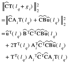
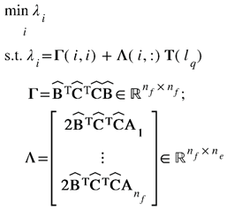
3. Simulation

In this section, we use simulations to validate key aspects of the generalized SmartScan approach presented in the foregoing sections. The first set of simulations presented in Section 3.1 demonstrates the benefits of imbuing SmartScan with global foresight. Then the second set of simulations numerically evaluates the benefits of SmartScan (including the global foresight) on a complex 3D part geometry that is tested in experiments in Section 4.

All the simulations employ an FDM model with an element height of Δz = 40 μm (the same as the layer thickness) and Δx = Δy = 200 μm, and Δt = 0.3 ms. As discussed in Section 2.1, the top surface of the parts is assumed to experience convective heat transfer, the side surfaces are insulated (by the powder) and the bottom surface is a Dirichlet boundary condition at the build plate temperature, T_b. The parts are all assumed to be made of AISI 316 L stainless steel using the process parameters provided in Table 1, which are based on the experimental set up introduced in Section 4. The material properties used for the simulations are also listed in Table 1 for AISI 316 L stainless steel under solidus conditions (where applicable). The material properties are assumed to be temperature independent in the simulations, to be consistent with the assumptions made in deriving the SmartScan algorithm. The experimental validation in Section 4 provides an avenue to test SmartScan under more realistic conditions, including temperature dependent parameters.

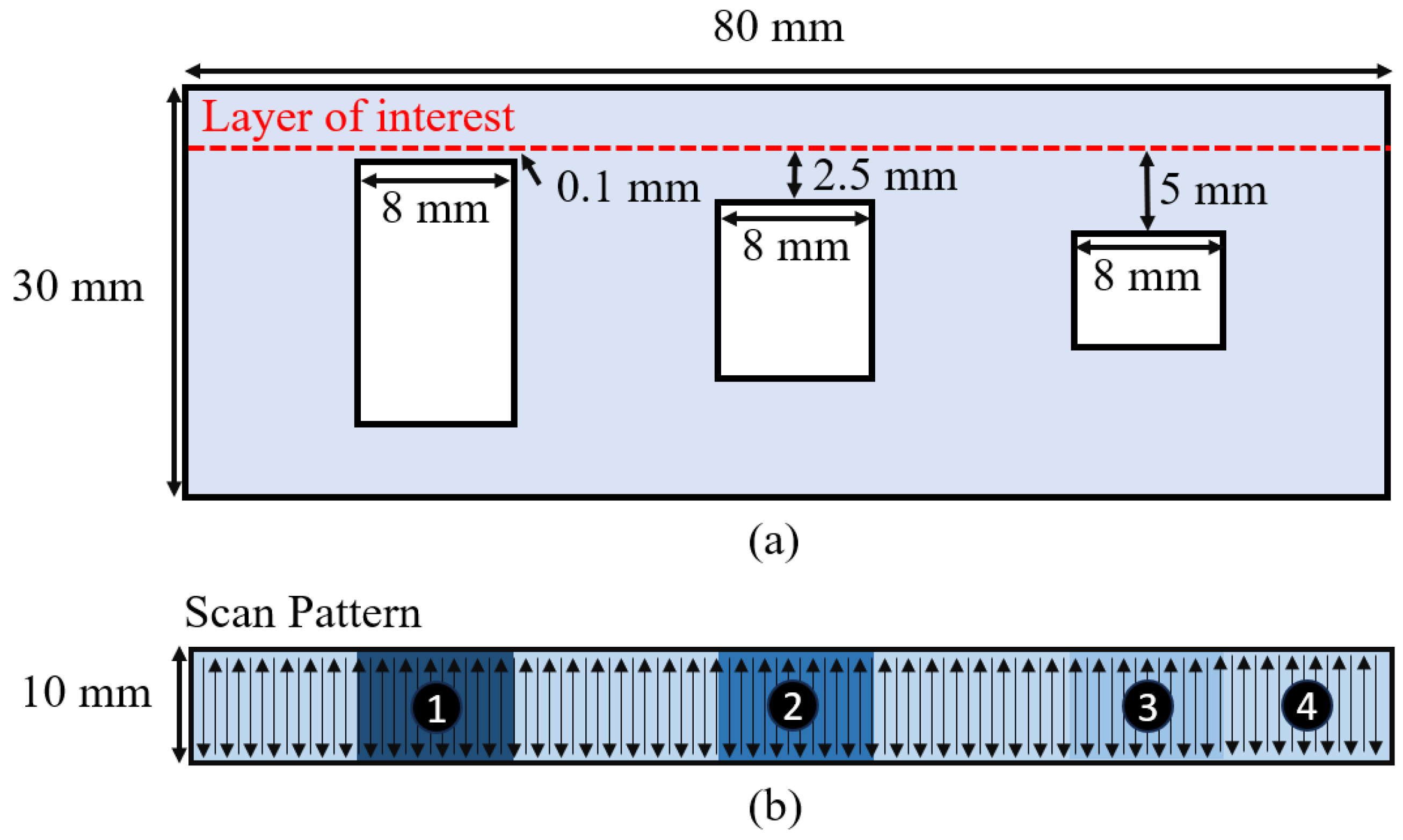
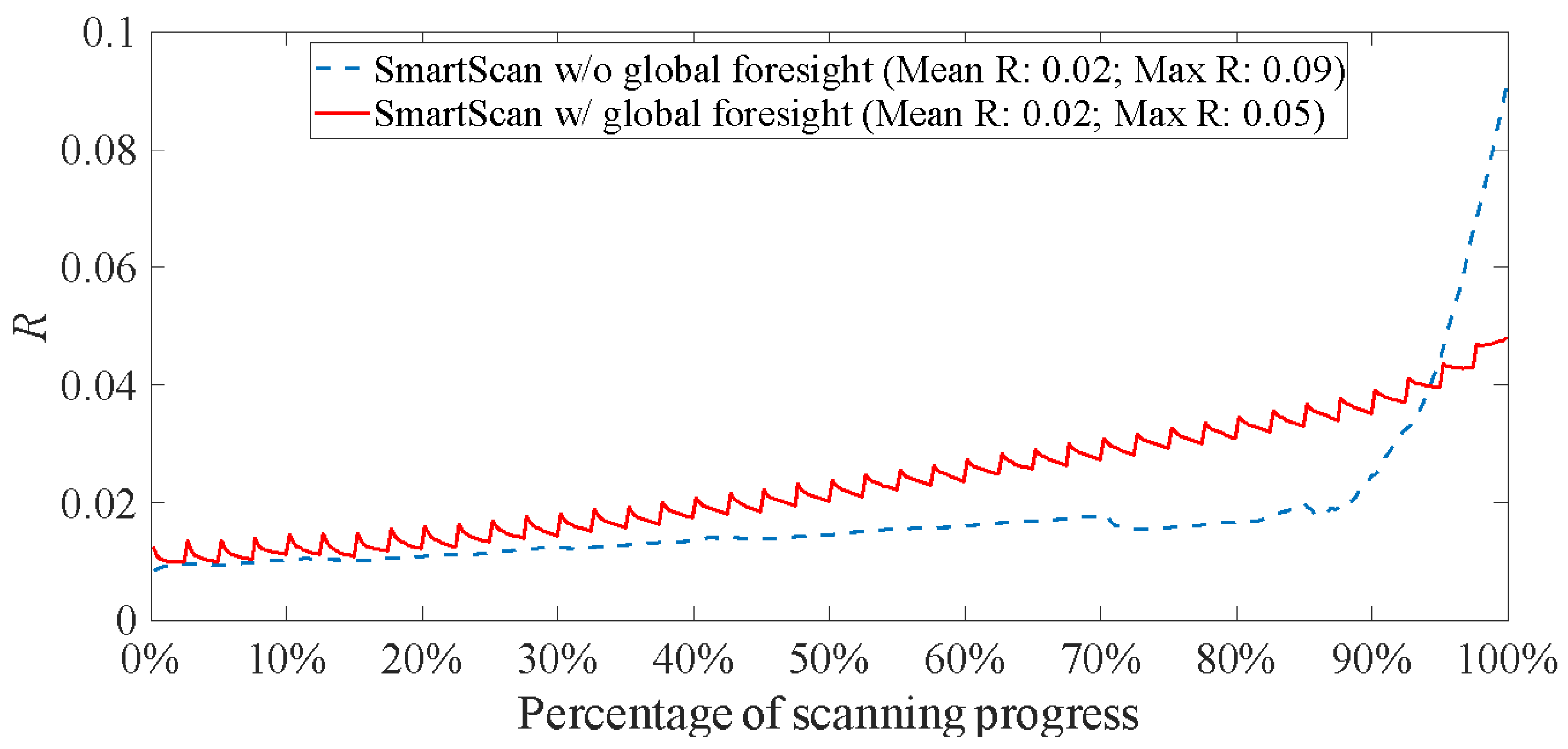
3.1. Evaluation of Global Foresight of SmartScan

Figure 8(a) depicts a side view of a 3D part geometry with overhangs of different sizes. All the layers of the part are hatched using vectors that are perpendicular to the long edge of the part, as shown in Figure 8(b). In our simulations, we focus on the layer that lies above all the overhangs and allows us to evaluate the benefit of providing SmartScan with global foresight.

Figure 8(b) shows how the layer of interest is segmented into four clusters based on heat conduction using the method described in Section 2.2.1; the clusters are numbered from 1 to 4 in increasing order of their thermal conductivity. Figure 9 shows the optimization results of SmartScan for the layer of interest in the presence and absence of the global foresight. Global foresight prevents the increase in R from being drastic and causing excessive local overheating. As a result, it reduces the maximum R value by 44.4% while maintaining the same mean R value as the case without global foresight. Therefore, in the rest of the simulations and experiments carried out in this paper, SmartScan includes global foresight even when it is not explicitly mentioned.

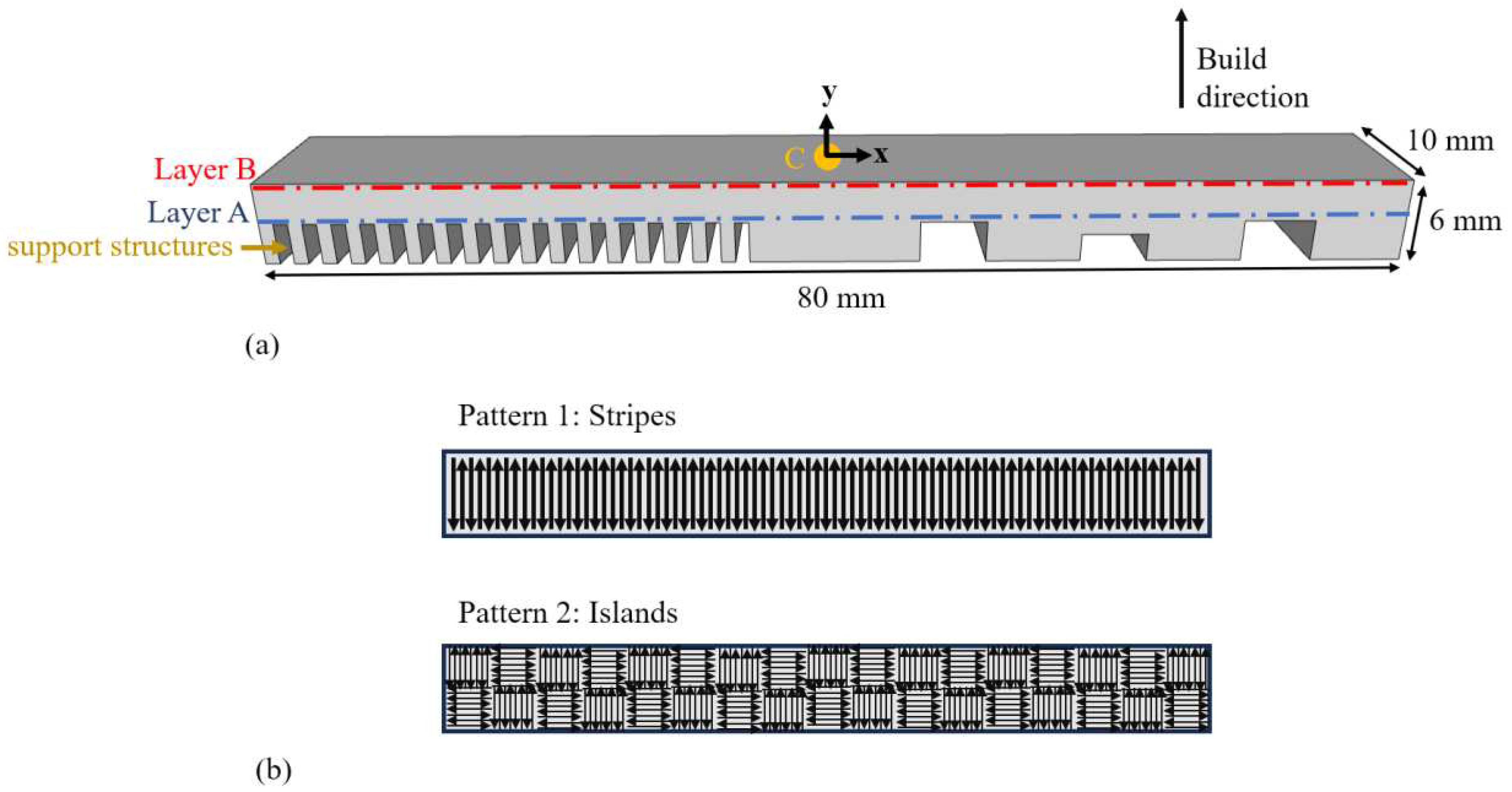
3.2. Simulation of Part Tested in Experiments

Figure 10(a) shows the part designed for validating the generalized SmartScan in experiments. It consists of three sections. The left side of the part is a cantilever beam supported by overhangs to test the effects of SmartScan on part deformation. The right side of the part includes overhangs for evaluating the impact of SmartScan on local heat accumulation. The center of the part features a solid block that is used to test the effects of SmartScan on residual stress. The purpose of the simulations carried out in this section is to evaluate the impact of SmartScan on thermal uniformity, compared to heuristic scan sequences, in advance of experiments in Section 4 focused on evaluating deformation, residual stress, and surface roughness. As shown in Figure 10(b), the part is evaluated using stripe and island scan patterns focusing on two layers: Layer A (the layer just above the overhangs) and Layer B (the topmost layer of the part).

3.2.1. Case 1: Stripe Scan Pattern

Here, the part in Figure 10(a) is simulated using the stripe scanning pattern, implementing a common practice of rotating the scan vectors of each layer by 67° relative to the preceding layer (Wang et al., 2023). To evaluate SmartScan, two prevalent heuristic sequences are used as benchmarks: Sequential (which involves scanning the stripes consecutively from one end of the part to the other), and Alternating (which first scans every other stripe consecutively, then returns to scan the remaining stripes consecutively to help distribute heat more evenly).

Firstly, we investigate Layer A (the layer just above the overhangs). Figure 11 displays the temperature uniformity metric, R, (as expressed in Eq. (3)) relative to the scanning progress percentage. SmartScan achieves 71% and 50% lower mean R than Sequential and Alternating, respectively, meaning that SmartScan delivers superior thermal uniformity compared to the benchmarks. This observation is confirmed in Figure 12 which presents the thermal distributions at four key stages—25%, 50%, 75%, and 100%—of scanning progress, with SmartScan generally exhibiting better temperature distribution. Notice that, even with its global foresight, SmartScan still exhibits a significant increase in R (i.e., thermal inhomogeneity) at the end of the scanning process. However, as demonstrated in Section 3.1, providing SmartScan with global foresight reduces the severity of the increased thermal inhomogeneity.

Secondly, we investigate the thermal uniformity of Layer B, the topmost layer of the part. Figure 13 depicts the temperature uniformity metric, R, again as a function of scanning progression. SmartScan exhibits mean R values that are lower than those of Sequential and Alternating by 93% and 88%, respectively. Accordingly, the temperature distributions shown in Figure 14 confirm SmartScan’s ability to provide better thermal uniformity compared to the heuristic methods.

3.2.2. Case 2: Island Scan Pattern

The part in Figure 10(a) is produced using the island scanning pattern, where, following the customary practice, the scan vectors are rotated by 90° between adjacent islands. The islands are each of size 5×5 mm². Two heuristic sequences are used as benchmarks. The first sequence is Chessboard (where the islands with horizontal vectors in Figure 10(b) are first scanned sequentially, followed by the islands with vertical vectors, much like the black and white squares in chess). The second sequence is Least Heat Influence (LHI), based on a tessellation algorithm (Maleki Pour, 2018), which maximizes the pairwise Euclidean distance between the upcoming scanned island and the previously scanned islands. Note that the supporting structures of all parts in this island case study adopted the standard chessboard scanning strategy.

Figure 15 illustrates the temperature uniformity metric, R, defined in Eq. (3) as a function of scanning progress percentage for Layer A. SmartScan results in 10% and 18% lower mean R than Chessboard and LHI, respectively. Figure 16 corroborates this observation, based on the thermal distribution at four stages—after 25%, 50%, 75%, and 100% of island scanning. SmartScan generally exhibits better thermal uniformity than the heuristic methods at all stages.

In Figure 17, the temperature uniformity metric, R, is presented as a function of scanning progression percentage for Layer B. SmartScan yields 8% and 18% lower mean R than Chessboard and LHI, respectively. This affirms that the proposed SmartScan technique offers enhanced thermal uniformity compared to the heuristic sequences. Furthermore, these findings are validated by Figure 18 which shows the improved thermal distribution of SmartScan at different points of scanning progress—at 25%, 50%, 75%, and 100% of island scanning.

Observe that the thermal uniformity (R) produced by SmartScan relative to the heuristic sequences is not as large as that obtained for the stripe pattern in Section 3.2.1. This is because the island pattern (with 32 islands) provides fewer degrees of freedom for optimization compared to the stripe pattern (with approximately 450 stripes).

4. Experiments

4.1. Experimental Setup and Procedure

The effectiveness of the generalized SmartScan was evaluated through experiments using the case studies presented in Sections 3.2.1 and 3.2.2. The parts were printed using the open-architecture PANDA 11 LPBF machine (from OpenAdditive, LLC, Beavercreek, OH) shown in Figure 19. It is equipped with a 500W IPG Photonics 1070nm fiber laser and a SCANLAB hurrySCAN galvo scanner with an F-theta lens. Controlled by the Open Machine Control software, it allows user-programmed custom scan patterns and sequences.

The parameters utilized for printing each specimen are given in Table 1. The parts were printed with AISI 316 L stainless steel powder sourced from Atlantic Equipment Engineers Company located in New Jersey. This particular stainless steel powder has a particle size described by D10 = 10-15 μm, D50 = 22-28 μm and D90 = 40-48 μm. A cross flow arrangement with nitrogen gas, at a regulated rate of 0.5–1.5 L/min, was used. The parts were built on top of an aluminum substrate measuring 152 mm × 152 mm in area, and 20 mm in height. Before starting the actual process of melting and solidifying the steel powder, the powder bed was not subjected to any preheating. After printing, the support structures (thin teeth) on the left of the part (see Figure 10(a)) were sawed off the build plate using a band saw. The top surface of the part was then scanned using the Romer Absolute Arm model #7525SI (Hexagon, Stockholm, Sweden), which has a 29 µm volumetric accuracy and 20 µm point repeatability. The resultant point clouds were transferred to MATLAB to extract information about the post-printing deformation of the parts. When the support structures were sawed off from the substrate, the upper surface of the part (Layer B) exhibited varying degrees of upward bending due to the release of some residual stress; these bending deformations were captured using the point clouds. Furthermore, the point clouds were used to assess the surface roughness of the part in portions of Layer B that did not experience post-build deformation (e.g., the center portion of the part in Figure 10(a)). Finally, a 10 x 10 x 4 mm³ specimen was extracted from the central section of the part by the band saw, at the location marked as “Point C” in Figure 10(a). A Cu-targeted X-ray diffraction machine (Rigaku Ultima IV XRD) was used for residual stress measurement of the specimen, and the machine’s proprietary PDLX software was used for data analysis. The machine was operated at 40 kV and 40 mA for measurements. The sin2ψ method was applied for the stress analysis with various tilt angles (−30°, −25°, −20°, −15°, −10°, 0°) for two series of samples and the elastic modulus was kept constant at 190 GPa while the Poisson ratio was taken 0.265 for each sample.

4.2. Results and Discussion

4.2.1. Deformation Analysis

Figure 20 shows the three printed parts (one for each of the scan sequences presented in Section 3.2.1) for the stripe pattern. Based on the measurement of the bending deformation of the cantilever beam portion (left side) of the part, SmartScan results in a 24.6% and 26.2% reduction in the maximum part deformation compared to Sequential and Alternating, respectively. Figure 21 shows the same test for the island pattern. SmartScan results in a 17.3% and 13.8% reduction in the maximum part deformation compared to Chessboard and LHI, respectively. While SmartScan does not completely eliminate deformation, its ability to reduce it could be very valuable in enabling parts to meet target tolerances. Moreover, it can be combined with other techniques, e.g., distortion pre-compensation (Afazov et al., 2017) to further reduce deformation and improve printed part quality.

Due to heat accumulation and the effects of gravity, a common defect that occurs at overhangs is a partial or total collapse of the overhang. This defect is seen for all three printed parts at the larger overhangs (i.e., Overhangs X and Z in Figure 20). However, because of the lower heat accumulation thanks to SmartScan (see Section 3.2.1), the craters caused by the collapse of the overhangs are 12.5% and 10.4% shallower for Overhangs X and Z, respectively, using SmartScan compared to Sequential. Similarly, as shown in Figure 20, the craters caused by the collapse of the overhangs are 22.2% and 12.2% shallower for Overhangs X and Z, respectively, using SmartScan compared to Alternating. A similar defect is recognizable across all three printed parts utilizing the island scan pattern as shown in Figure 21. However, the island scan pattern results in only one visible collapse (of the Z overhang). As with the stripe case, the use of SmartScan leads to a decrease in heat accumulation, causing a subsequent reduction in the depth of the collapse. Chessboard brings more serious defects, small protrusions, which may cause irreversible damage to the recoater blade. Also, as described in Figure 21, when SmartScan is applied, there is a 6.3% reduction in the depth of the crater caused by the collapsed Overhang Z, compared to the results from LHI.

Typically, the collapse at overhangs is mitigated by adding support structures and/or lowering the laser power at overhangs to reduce local overheating. In this case, none of these strategies were applied. However, the results show that SmartScan can reduce the need to lower laser power or add support structures, even when it cannot eliminate this need. SmartScan can be combined with the existing methods for reducing overhang collapse to achieve better overall print quality.

4.2.2. Residual Stress Analysis

Table 2 and Table 3 summarize the results of the residual stress measurements discussed in Section 4.1 using XRD. The measurements are taken in the x and y directions of a 5x5 mm² region of the 10 x 10 x 4 mm³ sample taken from Point C in Figure 10. For the stripe case, the use of SmartScan resulted in a 29.6% and 62.1% reduction of the x-component of residual stress, and a 54.6%, and 71.7% reduction in the y-direction of residual stress compared to Sequential and Alternating, respectively. Similarly, for the island pattern, SmartScan resulted in a 70.4% and 40.8% reduction of the x-component of residual stress, and an 86.7% and 84.2% reduction in the y-direction of residual stress compared to Chessboard and LHI, respectively. The large reductions in residual stress provided by SmartScan could be beneficial in practice because it decreases the risk of print failures directly caused by excessive stress during the printing process, before post-process stress relief. With lower as-built residual stress, the duration of the heat treatment process could also be shortened, which decreases the energy consumption of the post processing step.

4.2.3. Surface Roughness Analysis

Using the point cloud obtained from the upper surface of Layer B in Section 4.2.1, the roughness of the upper surface of each sample was measured as shown in Table 4. The roughness, R_a, is represented by the average deviation in the area. For the stripe pattern, SmartScan resulted in 9.5% and 20.3% higher R_a than Sequential and Alternating, respectively. For the island pattern, SmartScan yielded 1.3% and 4.0% higher R_a than Chessboard and LHI, respectively. A similar finding was made by Qin et al., (2023) using the 2D version of SmartScan. The implication is that, in most instances, SmartScan causes a small but significant increase in surface roughness compared to the heuristic sequences. A reason for this could be that the hopping around of the laser beam induced by SmartScan could cause some portions of the layer to be covered by spatter before they are scanned, as opposed the consecutive scanning where the deposition of spatter could be controlled to yield better surface finishes. However, this does not seem to be the only factor behind this observation because Alternating yields a better surface finish than Sequential, even though Sequential involves no jumping around of the laser while Alternating involves a little bit of jumping. Therefore, this matter requires further investigation, perhaps using a high-speed camera, to better understand the reasons for the slightly increased surface roughness using SmartScan.

4.2.4. Printing Time and Computational Cost Analysis

Table 5 shows the recorded print time for each sample obtained during the printing experiments. According to the data for the stripe pattern, SmartScan caused a 5.7% increase in print time compared to both Sequential and Alternating. However, in the case of the island pattern, SmartScan resulted in an equivalent print time as that of the Chessboard and LHI. This suggests that the use of SmartScan generally does not result in substantial increases in print time when compared to heuristic sequences. This can be credited to the laser’s jump speed being significantly faster than its scan speed.

In addition, the computation cost is also an important consideration for SmartScan, as it affects the practicality of the method. In the experiments reported above, SmartScan optimized each layer of the part within a minute using an AMD Ryzen 9 7945HX processor, 32.0 GB RAM and NVIDIA GeForce RTX 4070 Laptop GPU. The computational time of SmartScan is reasonable, as it is close to the interlayer time of LPBF. Its computational time can be further reduced by leveraging parallel computing and code optimization.

5. Conclusions and Future Work

In this paper, we have presented a generalized SmartScan methodology, which addresses critical challenges of thermal inhomogeneity, residual stress and distortion in parts made using laser powder bed fusion (LPBF) additive manufacturing. Our prior work introduced SmartScan, a novel method that harnessed model-based and optimization-driven principles to replace heuristics-based laser scan sequencing. However, it was limited to 2D geometries, leaving a significant gap in addressing the complexities of 3D structures. The generalized SmartScan proposed in this paper has been made applicable to arbitrary 3D part geometries by: (1) expanding the thermal model and optimization approach used in prior versions of SmartScan to multiple layers; (2) enabling SmartScan to process shapes with arbitrary contours and infill patterns within each layer and (3) providing SmartScan with global foresight to make it less myopic in its optimization.

The results obtained from the printing of sample 3D parts using the generalized SmartScan approach, compared to those produced using heuristic scan sequences yielded up to 93%, 87% and 26% reduction in temperature inhomogeneity, residual stress, and deformation – all critical factors impacting the quality and integrity of manufactured components. Notably, these improvements have been achieved within reasonable computational times (< 1 minute per layer) and without significantly sacrificing printing speed, reaffirming the practical viability of the proposed methodology. However, SmartScan resulted in minor increases in surface roughness (< 5%) using the island scan pattern, and significant increases in surface roughness (up to 20%) using the stripe scan pattern, compared to heuristic scan sequences. The increases in surface roughness were attributed, in part, to higher levels of spatter falling on the printed surfaces due to the laser jumping around from point to point.

Future research will investigate the impacts of SmartScan on part microstructure, porosity, and other defects or properties of the manufactured component that are influenced (either directly or indirectly) by scanning sequence.

References

- Afazov, S., Denmark, W. A. D., Lazaro Toralles, B., Holloway, A., & Yaghi, A. (2017). Distortion prediction and compensation in selective laser melting. Additive Manufacturing, 17, 15–22. [CrossRef]
- Ahmed, M., Seraj, R., & Islam, S. M. S. (2020). The k-means Algorithm: A Comprehensive Survey and Performance Evaluation. Electronics, 9(8), 1295. [CrossRef]
- Boissier, M., Allaire, G., & Tournier, C. (2022). Time Dependent Scanning Path Optimization for the Powder Bed Fusion Additive Manufacturing Process. Computer-Aided Design, 142, 103122. [CrossRef]
- Cao, S., Zou, Y., Lim, C. V. S., & Wu, X. (2021). Review of laser powder bed fusion (LPBF) fabricated Ti-6Al-4V: process, post-process treatment, microstructure, and property. Light: Advanced Manufacturing, 2(2), 1. [CrossRef]
- Cao, Y., Moumni, Z., Zhu, J., Gu, X., Zhang, Y., Zhai, X., & Zhang, W. (2023). Effect of scanning speed on fatigue behavior of 316L stainless steel fabricated by laser powder bed fusion. Journal of Materials Processing Technology, 319, 118043. [CrossRef]
- Chen, Q., Taylor, H., Takezawa, A., Liang, X., Jimenez, X., Wicker, R., & To, A. C. (2021). Island scanning pattern optimization for residual deformation mitigation in laser powder bed fusion via sequential inherent strain method and sensitivity analysis. Additive Manufacturing, 46, 102116. [CrossRef]
- Dong, G., Wong, J. C., Lestandi, L., Mikula, J., Vastola, G., Jhon, M. H., Dao, M. H., Kizhakkinan, U., Ford, C. S., & Rosen, D. W. (2022). A part-scale, feature-based surrogate model for residual stresses in the laser powder bed fusion process. Journal of Materials Processing Technology, 304, 117541. [CrossRef]
- Guo, C., Li, S., Shi, S., Li, X., Hu, X., Zhu, Q., & Ward, R. M. (2020). Effect of processing parameters on surface roughness, porosity and cracking of as-built IN738LC parts fabricated by laser powder bed fusion. Journal of Materials Processing Technology, 285, 116788. [CrossRef]
- He, C., & Okwudire, C. (2023). Scan Sequence Optimization for Reduced Residual Stress and Distortion in PBF Additive Manufacturing – An AISI 316L Case Study. In Proceedings of the Ground Vehicle Systems Engineering and Technology Symposium (GVSETS), NDIA, Novi, MI, Aug. 15-17, 2023.
- He, C., Ramani, K. S., & Okwudire, C. E. (2023). An intelligent scanning strategy (SmartScan) for improved part quality in multi-laser PBF additive manufacturing. Additive Manufacturing, 64, 103427. [CrossRef]
- He, C., Ramani, K. S., Tsai, Y.-L., & Okwudire, C. E. (2022). A Simplified Scan Sequence Optimization Approach for PBF Additive Manufacturing of Complex Geometries. 2022 IEEE/ASME International Conference on Advanced Intelligent Mechatronics (AIM), 1004–1009. [CrossRef]
- He, C., Tsai, Y.-L., & Okwudire, C. E. (2022, June 27). A Comparative Study on the Effects of an Advanced Scan Pattern and Intelligent Scan Sequence on Thermal Distribution, Part Deformation, and Printing Time in PBF Additive Manufacturing. In proceedings of the ASME 2022 17th International Manufacturing Science and Engineering Conference (MSEC), Jun. 2022. [CrossRef]
- Kaleli Alay, T., Cagirici, M., Yalcin, M. Y., Yagmur, A., Tirkes, S., Aydogan, E., & Gur, C. H. (2023). Tailoring the microstructure and mechanical properties of IN718 alloy via a novel scanning strategy implemented in laser powder bed fusion. Materials Science and Engineering: A, 884, 145543. [CrossRef]
- Khan, H. M., Karabulut, Y., Kitay, O., Kaynak, Y., & Jawahir, I. S. (2021). Influence of the post-processing operations on surface integrity of metal components produced by laser powder bed fusion additive manufacturing: a review. Machining Science and Technology, 25(1), 118–176. [CrossRef]
- Kim, S. I., & Hart, A. J. (2022). A spiral laser scanning routine for powder bed fusion inspired by natural predator-prey behaviour. Virtual and Physical Prototyping, 17(2), 239–255. [CrossRef]
- Kruth, J. P., Froyen, L., Van Vaerenbergh, J., Mercelis, P., Rombouts, M., & Lauwers, B. (2004). Selective laser melting of iron-based powder. Journal of Materials Processing Technology, 149(1–3), 616–622. [CrossRef]
- Kumar, V. P., & Jebaraj, A. V. (2023). Comprehensive review on residual stress control strategies in laser-based powder bed fusion process– Challenges and opportunities. Lasers in Manufacturing and Materials Processing, 10(3), 400–442. [CrossRef]
- Liu, F., & Deng, Y. (2021). Determine the Number of Unknown Targets in Open World Based on Elbow Method. IEEE Transactions on Fuzzy Systems, 29(5), 986–995. [CrossRef]
- Liu, Y., Li, J., Xu, K., Cheng, T., Zhao, D., Li, W., Teng, Q., & Wei, Q. (2022). An optimized scanning strategy to mitigate excessive heat accumulation caused by short scanning lines in laser powder bed fusion process. Additive Manufacturing, 60, 103256. [CrossRef]
- Mahmoodkhani, Y., Ali, U., Imani Shahabad, S., Rani Kasinathan, A., Esmaeilizadeh, R., Keshavarzkermani, A., Marzbanrad, E., & Toyserkani, E. (2019). On the measurement of effective powder layer thickness in laser powder-bed fusion additive manufacturing of metals. Progress in Additive Manufacturing, 4(2), 109–116. [CrossRef]
- Maleki Pour, E. (2018). Innovative Tessellation Algorithm for Generating More Uniform Temperature Distribution in the Powder-bed Fusion Process. [Master’s dissertation, Purdue University].
- Mugwagwa, L., Dimitrov, D., Matope, S., & Yadroitsev, I. (2019). Evaluation of the impact of scanning strategies on residual stresses in selective laser melting. The International Journal of Advanced Manufacturing Technology, 102(5–8), 2441–2450. [CrossRef]
- Ning, J., Sievers, D. E., Garmestani, H., & Liang, S. Y. (2019). Analytical Thermal Modeling of Metal Additive Manufacturing by Heat Sink Solution. Materials, 12(16), 2568. [CrossRef]
- Pant, P., Salvemini, F., Proper, S., Luzin, V., Simonsson, K., Sjöström, S., Hosseini, S., Peng, R. L., & Moverare, J. (2022). A study of the influence of novel scan strategies on residual stress and microstructure of L-shaped LPBF IN718 samples. Materials & Design, 214, 110386. [CrossRef]
- Parry, L., Ashcroft, I. A., & Wildman, R. D. (2016). Understanding the effect of laser scan strategy on residual stress in selective laser melting through thermo-mechanical simulation. Additive Manufacturing, 12, 1–15. [CrossRef]
- Qin, M., Qu, S., Ding, J., Song, X., Gao, S., Wang, C. C. L., & Liao, W.-H. (2023). Adaptive toolpath generation for distortion reduction in laser powder bed fusion process. Additive Manufacturing, 64, 103432. [CrossRef]
- Ramani, K. S., He, C., Tsai, Y.-L., & Okwudire, C. E. (2022). SmartScan: An Intelligent Scanning Approach for Uniform Thermal Distribution, Reduced Residual Stresses and Deformations in PBF Additive Manufacturing. Additive Manufacturing, 102643. [CrossRef]
- Ramos, D., Belblidia, F., & Sienz, J. (2019). New scanning strategy to reduce warpage in additive manufacturing. Additive Manufacturing, 28, 554–564. [CrossRef]
- Reiff, C., Bubeck, W., Krawczyk, D., Steeb, M., Lechler, A., & Verl, A. (2021). Learning Feedforward Control for Laser Powder Bed Fusion. Procedia CIRP, 96, 127–132. [CrossRef]
- Riensche, A., Bevans, B. D., Smoqi, Z., Yavari, R., Krishnan, A., Gilligan, J., Piercy, N., Cole, K., & Rao, P. (2022). Feedforward control of thermal history in laser powder bed fusion: Toward physics-based optimization of processing parameters. Materials & Design, 224, 111351. [CrossRef]
- Sames, W. J., List, F. A., Pannala, S., Dehoff, R. R., & Babu, S. S. (2016). The metallurgy and processing science of metal additive manufacturing. International Materials Reviews, 61(5), 315–360. [CrossRef]
- Wang, R., Standfield, B., Dou, C., Law, A. C., & Kong, Z. J. (2023). Real-time process monitoring and closed-loop control on laser power via a customized laser powder bed fusion platform. Additive Manufacturing, 66, 103449. [CrossRef]
- Wang, Z., Yang, Z., Liu, F., & Zhang, W. (2023). Influence of the scanning angle on the grain growth and mechanical properties of Ni10Cr6W1Fe9Ti1 HEA fabricated using the LPBF–AM method. Materials Science and Engineering: A, 864, 144596. [CrossRef]
- Wei, L. C., Ehrlich, L. E., Powell-Palm, M. J., Montgomery, C., Beuth, J., & Malen, J. A. (2018). Thermal conductivity of metal powders for powder bed additive manufacturing. Additive Manufacturing, 21, 201–208. [CrossRef]
- Yang, H., Sha, J., Zhao, D., He, F., Ma, Z., He, C., Shi, C., & Zhao, N. (2023). Defects control of aluminum alloys and their composites fabricated via laser powder bed fusion: A review. Journal of Materials Processing Technology, 319, 118064. [CrossRef]