Generalized SmartScan: An Intelligent LPBF Scan Sequence Optimization Approach for 3D Part Geometries

Preprint

Article

Generalized SmartScan: An Intelligent LPBF Scan Sequence Optimization Approach for 3D Part Geometries

This version is not peer-reviewed.

Chuan He

,Nathaniel Wood,Bircan Bugdayci,

Chinedum Okwudire^*

Chuan He

,Nathaniel Wood,Bircan Bugdayci,

Chinedum Okwudire^*

This version is not peer-reviewed.

Altmetrics

Downloads

505

Views

614

Comments

Submitted:

18 July 2024

Posted:

18 July 2024

You are already at the latest version

A peer-reviewed article of this preprint also exists.

Abstract

Laser powder bed fusion (LPBF) is an additive manufacturing technique that is gaining popularity for producing metallic parts in various industries. However, parts produced by LPBF are prone to residual stress, deformation, cracks and other quality defects due to uneven temperature distribution during the LPBF process. To address this issue, in prior work, the authors have proposed SmartScan, a method for determining laser scan sequence in LPBF using an intelligent (i.e., model-based and optimization-driven) approach, rather than using heuristics, and applied it to simple 2D geometries. This paper presents a generalized SmartScan methodology that is applicable to arbitrary 3D geometries. This is achieved by: (1) expanding the thermal model and optimization approach used in SmartScan to multiple layers; (2) enabling SmartScan to process shapes with arbitrary contours and infill patterns within each layer; (3) providing the optimization in SmartScan with a balance of exploration and exploitation to make it less myopic; and (4) improving SmartScan's computational efficiency via model order reduction using singular value decomposition. Sample 3D test artifacts are simulated and printed using SmartScan in comparison with common heuristic scan sequences. Reductions of up to 92% in temperature inhomogeneity, 86% in residual stress, 24% in maximum deformation and 50% in geometric inaccuracy were observed using SmartScan, without significantly sacrificing print speed. An approach for using SmartScan for printing complex 3D parts in practice, by integrating it as a plug-in to a commercial slicing software, was also demonstrated experimentally, along with its benefits in significantly improving printed part quality.

Keywords:

Subject:

Engineering - Industrial and Manufacturing Engineering

1. Introduction

Laser powder bed fusion (LPBF) is a prominent technique within the field of additive manufacturing (AM) of metals that is finding applications across diverse industries, including aerospace, automotive, and biomedical. This method employs high-intensity lasers to systematically melt powder, layer by layer, resulting in the creation of intricate 3D objects. Compared to other metal AM techniques, LPBF excels in fabricating complex parts with high precision at relatively high build speeds [1,2]. Nevertheless, LPBF-produced parts are susceptible to residual stress, deformation, and related defects stemming from non-uniform thermal distribution [3,4]. While post-process heat treatments can ameliorate some of these issues, they are often time-consuming, costly [5], and insufficient in rectifying deformation or cracks induced by thermal stresses during the build process [6,7,8]. Consequently, it is critical to minimize temperature gradients during the build process to assure quality [9].

Numerous studies have highlighted the critical role of scanning (or scan) strategy in achieving uniform temperature distribution and defect-free printing via LPBF. The umbrella term “scan strategy” encompasses a variety of approaches for altering scanning parameters, such as beam power, scan speed, hatch distance, scan pattern, and layer thickness. For instance, extensive research studies [10,11,12,13] have investigated altering laser power or speed, while others [14,15,16] have reported on the optimization of hatch distance. Additionally, many researchers [17,18,19,20,21,22,23,24] have explored scan path optimization with the aim of minimizing thermal gradients and distortion in LPBF.

Scan sequence, which is another integral component of scan strategy, has garnered increasing attention as a means to reduce thermal gradients and enhance print quality in LPBF. Scan sequence refers to the order in which the repeating geometric units of a scan pattern are traced by the laser. The repeating units (hereafter referred to as the "features") of a scan pattern could be, for example, the individual vectors of a bidirectional (zigzag) scan pattern or the islands of a chessboard scan pattern. Several studies have shown that scan sequence significantly impacts temperature uniformity, residual stress, and distortion in parts produced via LPBF [25,26,27,28]. Consequently, various methods have been proposed to determine scan sequences that minimize thermal gradients, residual stress, and distortion. For example, Kruth et al. [28] proposed the LHI, least heat influence, approach that begins by scanning a randomly selected feature and then continues by scanning the feature that is least heated (farthest away from the preceding feature). A similar approach to LHI was adopted by Qin et al. [20] who proposed a scan sequence algorithm for an island-based strategy that chose the island with the maximum distance from the currently active island until all islands had been traversed. Mugwagwa et al. [25] evaluated four scan sequences, namely, island, successive, successive chessboard, and LHI, in terms of their impact on residual stress and distortion, demonstrating that the choice of scan sequence resulted in the reduction of maximum distortion by up to 14% and the reduction in residual stress by up to 40%. Pant et al. [29] investigated sectional strategies that divided layers into three separate sections and scanned either the outermost section or the innermost section first for each layer, leading to the lowest residual stress levels among all the samples studied. Ramos et al. [27] proposed an intermittent scan sequence for the island scan pattern. Their method avoided scanning adjacent islands consecutively by using a geometry-based formula having weights and radial thresholds. Using their strategy, they demonstrated a 10% reduction in deformation compared to an alternating scan sequence, for the same vector length. Recently, Yang et al. [30] proposed the interval island technique, which was found to be more effective than the traditional stripe and continuous laser-scanning strategies because it resulted in smaller grain sizes, less thermal deformation, and lower residual stress anisotropy. Qin et al. [23] developed a deep reinforcement learning based toolpath generation framework for the LPBF process that could effectively reduce thermal accumulation and distortion by avoiding sensitive regions with high turning angles.

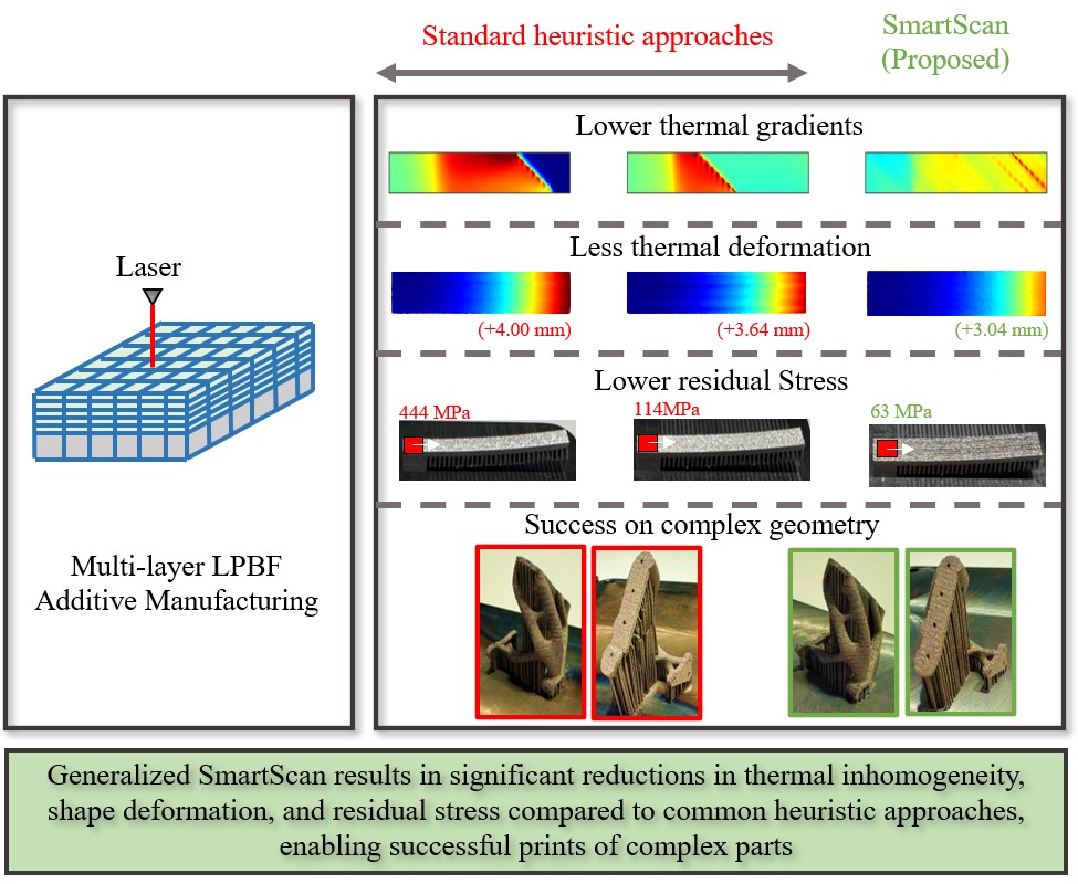
As noted in the authors’ earlier work [31], a deficiency shared by most of the existing methods for scan sequence generation is that they are highly dependent on heuristic formulations that approximate heat transfer in LPBF using geometric relationships that do not generalize well. To address this shortcoming, Ramani et al. [31] introduced SmartScan, an intelligent scan sequence generation approach for LPBF. SmartScan differentiates itself from heuristic techniques by utilizing thermal models of LPBF combined with rigorous control-based techniques to determine optimal scan sequences, facilitating its generalizability. The application of SmartScan to laser marking of AISI 316 L stainless steel plates demonstrated up to 41% and 47% reductions in thermal inhomogeneity and distortion, respectively, compared to state-of-the-art heuristic methods [31]. Moreover, SmartScan exhibited notable robustness and computational efficiency, making it suitable for online implementation. Subsequent work has expanded SmartScan to encompass complex geometries [32] and advanced scan patterns [33], and multi-laser PBF systems [34]. However, these prior works were limited to laser marking of 2D part geometries and lacked the capability to handle LPBF of 3D parts with arbitrary scan patterns and geometric features. To address these limitations, building on preliminary work [35], this paper introduces a generalized SmartScan algorithm applicable to LPBF of arbitrary 3D parts. The paper makes the following original contributions to the literature (see Figure 1):

It extends the 2D thermal model and objective function of the original SmartScan [31] to incorporate 3D thermal effects, while introducing simplifying assumptions to reduce computational complexity due to larger model sizes.
It generalizes the modeling and optimization methods of the original SmartScan to enable them to handle arbitrary scan patterns with scan vectors of varying lengths and inclination angles within each layer.
It improves the original SmartScan’s greedy optimization strategy, which was prone to getting stuck in local optima, by balancing exploration and exploitation. This enables more efficient optimization of temperature distribution for part geometries with overhangs or other heat traps.
It further reduces the dimension of the model significantly, thereby enhancing computational efficiency by using singular value decomposition (SVD).

It validates the effectiveness of the generalized SmartScan through simulations and experiments involving the printing of two 3D test artifacts. The results demonstrate significantly reduced thermal inhomogeneity, residual stress, and distortion compared to commonly-used heuristic scan sequences. Moreover, it experimentally demonstrates an approach for using the generalized SmartScan for printing complex 3D parts in practice, along with its benefits in significantly improving printed part quality, by integrating SmartScan as a plug-in to a commercial slicing software.

The remainder of this paper is organized as follows: Section 2 broadens the scope of SmartScan to multi-layer LPBF with arbitrary geometric features and scan patterns, and improves the effectiveness and computational efficiency of the optimization algorithm of SmartScan. Section 3 presents simulation and experimental case studies to compare the thermal distribution, residual stress, distortion, and printing time achieved using SmartScan with those achieved with commonly-used heuristic scan sequences on 3D test artifacts. Section 3 also demonstrates an approach for using SmartScan to print complex 3D parts by embedding it as a plug-in to a commercial slicer. The paper concludes with Section 4, which summarizes the key findings and outlines avenues for future research.

2. Methodology

2.1. Extension of FDM Modeling to Arbitrary 3D Geometries and Scan Patterns

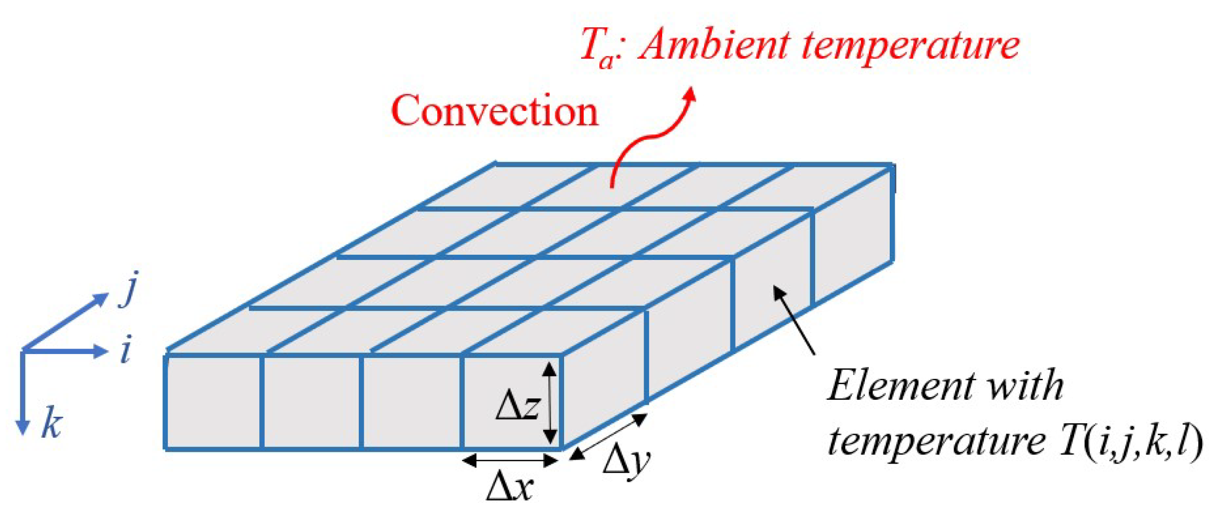
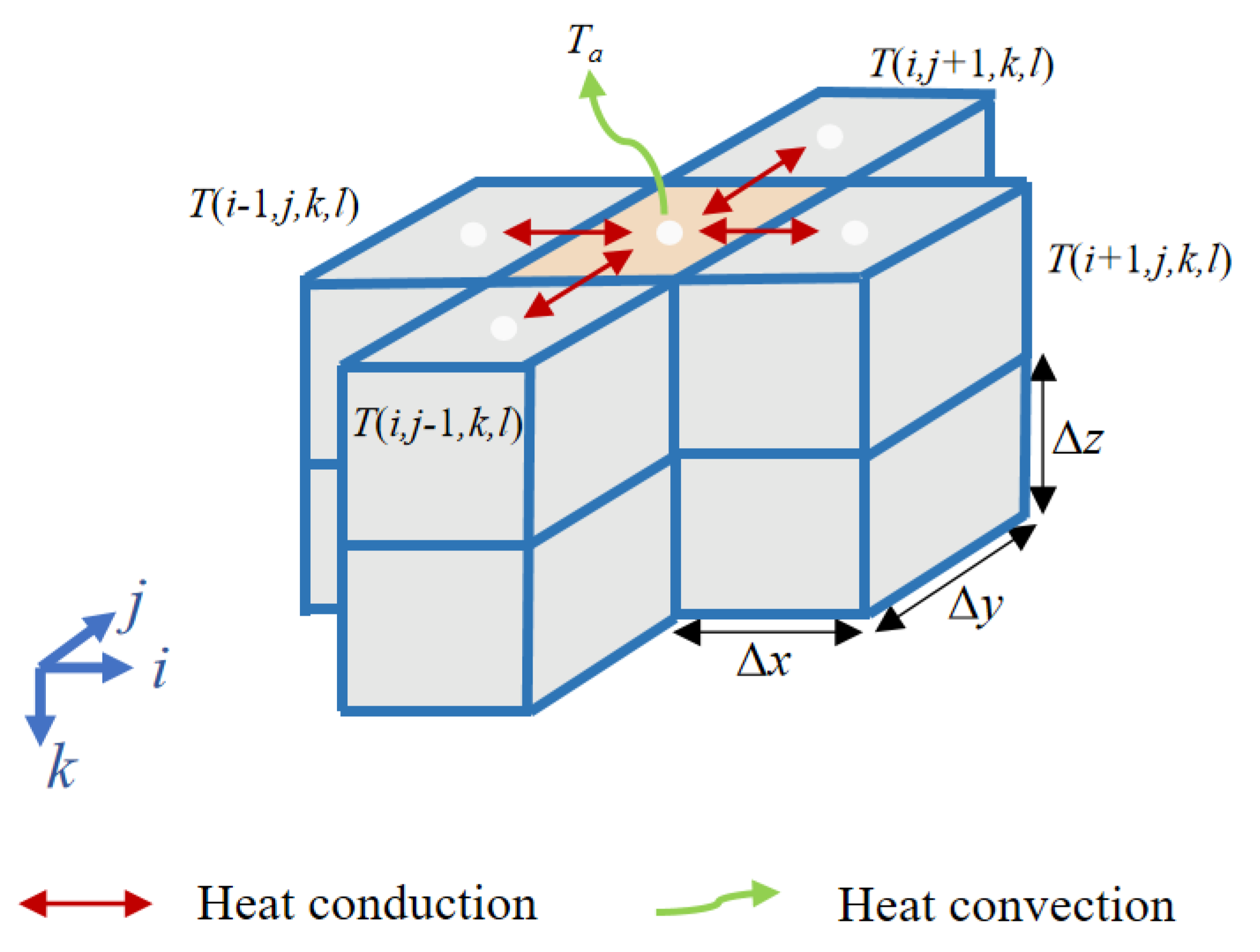
This section provides the underlying thermal model to handle 3D geometries with multiple layers. As in our prior work [31], we adopt a model that considers only conductive and convective heat transfer between the part being printed and its surroundings (See Figure 2). Radiative heat transfer, latent heat effects, Marangoni convection, and other melt pool phenomena, are ignored. These assumptions are reasonable because SmartScan focuses on part-scale temperature distribution; similar assumptions have been used in other works [36,37]. The model parameters are assumed to be temperature-independent to keep the model linear, which is critical for efficient optimization. In our prior work [31], we have demonstrated that this simplification does not significantly diminish the effectiveness of SmartScan. Accordingly, heat transfer within the printed part with conductivity

k_{t}

and diffusivity

α

can be described using the equation:

\frac{\partial^{2} T}{\partial x^{2}} + \frac{\partial^{2} T}{\partial y^{2}} + \frac{\partial^{2} T}{\partial z^{2}} + \frac{u}{k_{t}} = \frac{1}{α} \frac{\partial T}{\partial t}

(1)

where T is the temperature, x, y and z are the spatial coordinates, t is time and u is the power per unit volume. The finite differences method (FDM) can be used to discretize Eq.(1) to obtain

\begin{matrix} \frac{T (i + 1, j, k, l) + T (i - 1, j, k, l) - 2 T (i, j, k, l)}{Δ x^{2}} \\ + \frac{T (i, j + 1, k, l) + T (i, j - 1, k, l) - 2 T (i, j, k, l)}{Δ y^{2}} \\ + \frac{T (i, j, k + 1, l) + T (i, j, k - 1, l) - 2 T (i, j, k, l)}{Δ z^{2}} \\ + \frac{u (i, j, k, l)}{k_{t}} = \frac{1}{α} \frac{T (i, j, k, l + 1) - T (i, j, k, l)}{Δ t} \end{matrix}

(2)

where

Δ x

Δ y

and

Δ z

are the dimensions of each element (see Figure 2), i, j and k are the spatial indices of the elements, l is the temporal index (i.e., t = l

Δ t

Δ t

is the time step and T(i,j,k,l) is the temperature of the element located at (i,j,k) at time l. Without loss of generality, the element height

Δ z

is assumed to be equal to the layer height of the LPBF process, such that k serves as an index for deposited layers (referenced to the topmost fully-scanned layer where k = 1).

Two main factors must be considered in extending the 2D thermal model used in our prior work [31] to 3D, namely: (1) a powder layer and (2) multiple printed layers underneath the powder layer. The powder can be considered as an insulator since its conductivity is roughly an order of magnitude lower than that of solid metal [38]. However, during printing, the conductivity of the powder layer changes continuously as portions of it are converted from powder into solid metal. This means that some conductive heat transfer is bound to occur within the powder layer, resulting in a time-varying thermal model. However, the intra-layer conductivity variation of the powder layer is negligible since the powder layer is very thin (typically 20 to 100

μ m

[39]). Hence, most of the heat transfer that affects macro-scale temperature distribution occurs due to conduction into the layers below rather than within the powder layer; some heat is also lost to convection.

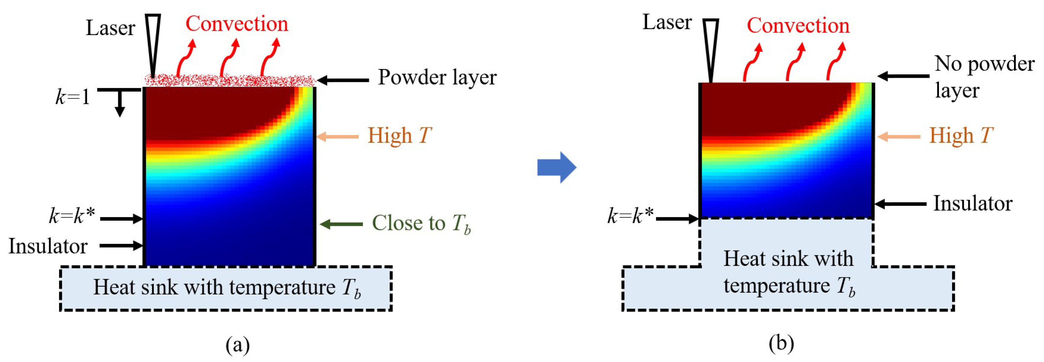
Therefore, for the sake of simplicity, we neglect the powder layer in our model (by treating it as a transparent layer) and apply the laser power directly to the layer beneath the powder, as shown in Figure 3. Additionally, the substrate (base plate) is assumed to function as a heat sink held at a constant, uniform temperature

T_{b}

. The sides of the part are insulated by the low-conductivity powder, and heat is lost by convection through the top layer. As layers are built during the printing process, the heat from the laser is conducted down into the substrate. Consequently, the layer-wise mean temperature can be expected to approach

T_{b}

at a certain layer

k = k^{*}

from the top surface. Since SmartScan focuses on maintaining a uniform temperature distribution rather than modeling the absolute temperature, the model can be simplified by replacing the layers

k > k^{*}

with a heat sink at a uniform temperature

T_{b}

. One benefit of this approximation is that the model size can be reduced to only consider layer numbers 1 ≤k≤

k^{*}

, as shown in Figure 3(b). The validity of this assumption is demonstrated using a characteristic example in the Appendix A, where it is shown that

k^{*} = 20

is a reasonable choice in a conservative scenario; hence it is used in the rest of this paper.

Based on the simplifications to the 3D thermal model discussed above, Equation (2) can be rearranged into a state space equation

T (l + 1) = AT (l) + Bu (l)

(3)

Here,

T

(l) refers to the state vector, encapsulating the thermal information T(i,j,k,l) for all elements in the region 1 ≤k≤

k^{*}

at time l. The state matrix is denoted by

A

, while

B

is the input matrix. The explicit generation of matrices

A

and

B

for arbitrary geometric shapes and scanning patterns, as well as the selection of parameters in the FDM model, such as grid size

Δ x

Δ y

and

Δ z

and sampling time

Δ t

, are demonstrated in Appendix B. The sparse vector

u

(l) denotes the power input; its non-zero elements coincide with the application location of the laser. The influence of heat transfer through convection to the ambient temperature

T_{a}

, with the convection coefficient h, and conduction to the layers below

k^{*}

with a temperature of

T_{b}

are incorporated into the model following the heat sink approach described [40]. Also, the laser beam’s heat flux is characterized by a Gaussian distribution [27].

Features within predetermined scan patterns refer to specific repeated elements whose scan sequence can be manipulated. In the context of unidirectional or bidirectional (zigzag) scanning, the features are vectors that are the linear paths. Similarly, in chessboard scanning or a similar fragment-based scanning strategy, the scan area is divided into regions. Each island or fragment can be considered as a feature. With the part-level state-space model in Equation (3) derived for any arbitrary geometry and scan pattern, the corresponding representation of the state-space at the feature level can be expressed.

To do this, let the features in any given layer be labeled 1, 2, …,

n_{F}

, and let

g_{f}

be the set of all time steps associated with feature f, i.e.

g_{f} = \{l_{f, 0}, l_{f, 1}, \dots, l_{f, N_{f} - 1}\}

. The feature f has

N_{f}

time steps to be traced by the laser. After the feature f is scanned (

f \in {1, 2, \dots, n_{F}}

), the corresponding feature-level state-space representation can be written as:

\begin{matrix} T (l_{q} + N_{f}) = A_{f} T (l_{q}) + b_{f} \\ A_{f} ≜ A^{N_{f}}; b_{f} ≜ \sum_{m = 0}^{N_{f} - 1} A^{N_{f} - 1 - m} B u (l_{f, m}); l_{q} = \sum_{f in SF (l_{q})} N_{f} \end{matrix}

(4)

where

l_{q}

is feature-level time index, which is set to

l_{q} = 0

at the beginning of each layer, and

SF (l_{q})

refers to the set of scanned features of each layer at time step

l_{q}

. Note that

l_{f, 0} = l_{q}

for each feature being scanned.

2.2. Objective Function and Optimization

As the objective function for optimization, the temperature uniformity metric R(k,l) [31] is used:

R (k, l) = \sqrt{\frac{\sum_{i, j} {(T (i, j, k, l) - T_{a v g} (k, l))}^{2}}{n_{k} T_{m}^{2}}}

(5)

where

T_{avg}

(k,l) denotes the mean of the temperatures T(i,j,k,l) of a layer k at time l,

n_{k}

signifies the number of elements of the corresponding layer k, and

T_{m}

represents the melting point of the material, which is used to normalize R.

SmartScan generates the optimal scan sequence while ensuring that each feature is scanned once and only once to minimize temperature inhomogeneity for each printed layer. This is achieved by minimizing the temperature uniformity metric R(1,

l_{q} + N_{f}

) of the topmost layer of our model, which can be written as

R (1, l_{q} + N_{f}) = {∥C T (l_{q} + N_{f})∥}_{2}; C = \frac{1}{\sqrt{n_{k}} T_{m}} [I - \frac{1 1^{T}}{n_{k}} 0]

(6)

where

1

represents a column vector of length

n_{k}

whose all elements are equal to 1,

I

is an identity matrix, and the

0

(null) matrix in the

C

matrix indicates that for the elements of

T

beyond the first layer,

T_{b}

and the ambient temperature

T_{a}

do not contribute to the calculation of R. Based on the feature-level state-space representation in Equation (4) and the temperature uniformity metric in Equation (6), the optimization problem for a layer k can be written as:

\begin{matrix} \arg min_{f} (R (1, l_{q} + N_{f}) = {∥C T (l_{q} + N_{f})∥}_{2}) \\ s . t . T (l_{q} + N_{f}) = A_{f} T (l_{q}) + b_{f} \end{matrix}

(7)

This optimization problem in Equation (7) is further written as:

\begin{matrix} | | CT (l_{q} + N_{f}) {| |}_{2}^{2} \\ = | | C A_{f} T (l_{q}) + C b_{f} {| |}_{2}^{2} \\ = b_{f}^{'} C^{'} C b_{f} \\ + 2 T^{'} (l_{q}) A_{f}^{'} C^{'} C b_{f} \\ + T^{'} (l_{q}) A_{f}^{'} C^{'} C A_{f} T (l_{q}) \end{matrix}

(8)

As such, the optimization takes the form:

\begin{matrix} \begin{matrix} \arg min_{f} λ_{f} \\ s . t . λ_{f} = β_{f} + γ_{f} T (l_{q}) + T^{'} (l_{q}) δ_{f} T (l_{q}) \\ β_{f} ≜ b_{f}^{'} C^{'} C b_{f} \\ γ_{f} ≜ 2 b_{f}^{'} C^{'} C A_{f} \\ δ_{f} ≜ A_{f}^{'} C^{'} C A_{f} \end{matrix} \end{matrix}

(9)

where

β_{f}

γ_{f}

and

δ_{f}

can be calculated in advance for every feature

f \in {1, 2, \dots, n_{F}}

The flowchart below summarizes the generalized SmartScan strategy.

Remark: Notice that the formulation of the feature-level state space equation in Equation (4) and the optimization in Equation (7) allows a variable number of time steps

N_{f}

per feature. This allows the generalized SmartScan algorithm to accommodate features of different sizes, which was not possible in the original SmartScan algorithm [31,34]), thus increasing its versatility to handle complex 3D geometries.

2.3. Relaxation of the Greediness of the Optimization Algorithm

An apparent problem with the SmartScan optimization algorithm, as described in Section 2.2 above (and in our prior work [31,34]) is that it is greedy. It minimizes R(1,

l_{q}

) for any given feature without a global foresight of the impact of its current actions on future outcomes. This means that it can result in premature convergence to suboptimal solutions due to inadequate exploration of the search space. This limits its effectiveness for complex 3D shapes.

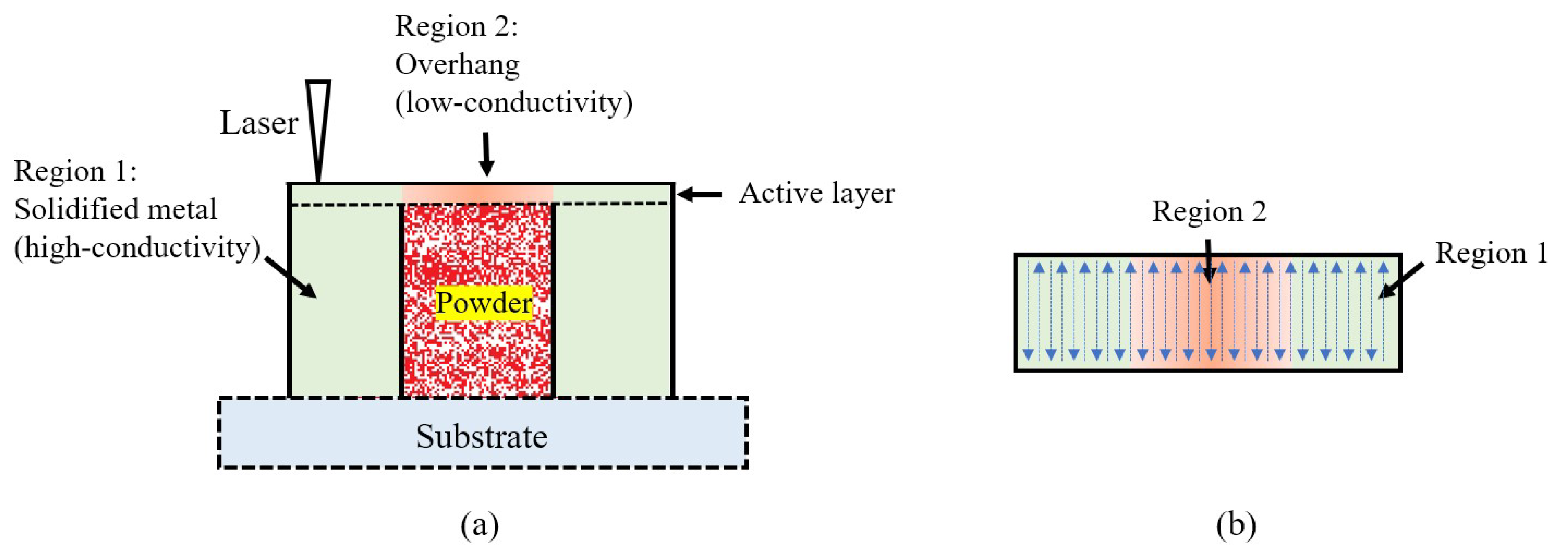
To illustrate this problem, consider a part with an overhang whose cross-section is shown in Figure 5(a). The part has a uniform depth into the page. At the print stage shown in the figure, the part can be divided into two regions – Region 1 supported by high-conductivity solid metal and Region 2 supported by low-conductivity powder. In optimizing the sequence of the vectors in the active layer shown in Figure 5(b), the shortsighted SmartScan algorithm would prioritize scanning the vectors in Region 1 because they yield lower R(1,

l_{q}

) values by conducting heat quickly to the bottom layers. Therefore, at the end, the algorithm is left with most of the vectors from Region 2 to scan, leading to extremely inhomogeneous thermal distribution and overheating of Region 2 toward the end of the scanning process.

In this section, we address this limitation of SmartScan by the integration of Gaussian distributed probability into the decision-making process of the greedy algorithm. This method is popular in reinforcement learning as a simple and effective way to address the balance between exploitation and exploration[41,42]. At a high level, the proposed solution modifies the SmartScan solution in Equation (9) where

λ_{m i n}

, the smallest value of

λ

is selected. Instead, it uses all the

λ

values to establish a Gaussian distribution from which the optimal

λ

is selected probabilistically, with higher probabilities placed on the smaller

λ

values. This makes the optimization less greedy by allowing it to balance exploitation (of the smaller

λ

values) with exploration of other

λ

values. In the context of the simple example in Figure 5(b), that means that more vectors in region 2 will be scanned earlier on due to a Gaussian distributed probability. These steps are detailed below.

In Equation (9), by obtaining all

λ_{f}

values corresponding to the

n_{F}

features within a layer k, the mean value

μ

and standard deviation

σ

that characterize the Gaussian distribution can be initialized as:

\begin{matrix} μ ≜ λ_{\min} \\ σ ≜ \sqrt{\frac{1}{n_{F}} Σ_{f = 1}^{n_{F}} {(λ_{f} - λ_{avg})}^{2}} \end{matrix}

(10)

where

λ_{\min}

and

λ_{avg}

refer to the minimum and average of

λ_{f}

values, respectively.

A probability

p_{f}

for each

λ_{f}

in Equation (9) using the Gaussian distribution centered at

μ

in Equation (10) can be calculated as:

p_{f} = \frac{1}{σ \sqrt{2 π}} e^{- \frac{{(λ_{f} - μ)}^{2}}{2 σ^{2}}}

(11)

Based on the calculated probabilities

p_{f}

, the feature to be scanned is selected by the roulette wheel method [43]. In Equation (10), the magnitude of the standard deviation

σ

dynamically controls the balance between exploitation and exploration. For example, on a layer without any overhang, where all

λ_{f}

values are fairly close in magnitude, a smaller

σ

reduces exploration, making it similar to the original (greedy) SmartScan described in Section 2.2. In the case of one or more overhangs, where

λ_{f}

values vary significantly, a larger

σ

enhances exploration.

2.4. SVD-based Model Order Reduction

Although some of the simplifying assumptions in Section 2.1 have significantly reduced the model size in Equation (3), the model size can still become very large when dealing with 3D printed components, leading to computationally intensive and sometimes infeasible calculations. To address this issue, we propose the use of a singular value decomposition (SVD)-based model reduction method to reduce the dimensionality of the model in Equation (3). SVD-based model reduction offers a significant advantage in computational efficiency for large-scale systems by constructing a reduced model that retains the key dynamic characteristics of the original system.

The reduced temperature vectors and system matrices are given by:

\begin{matrix} \tilde{T} = Φ^{'} T; \tilde{A} = Φ^{'} A Φ; \tilde{B} = Φ^{'} B; \tilde{C} = Φ^{'} C Φ \end{matrix}

(12)

where

\tilde{A}

\tilde{B}

and

\tilde{C}

are the reduced state, input and output matrices, respectively, and

Φ

is a

n_{e} \times n_{r}

projection matrix, where

n_{e}

and

n_{r}

represent the dimension of the full-scale model and the reduced model, respectively. The SVD of the matrix

A

can be computed as

U Σ V^{'}

. If the eigenvalues in

Σ

are arranged in descending order, the first

n_{r}

columns of

V

can be used as

Φ

. The columns in

Φ

consists of the vectors representing the most dominant dynamics of the system, ensuring that the main characteristics of the original system are preserved during this process.

This results in a new, lower-dimensional system reduced from a high-dimensional system in Equation (3):

\begin{matrix} \tilde{T} (l + 1) = \tilde{A} \tilde{T} (l) + \tilde{B} u (l); \\ \tilde{T} (0) = Φ^{'} T (0) \end{matrix}

(13)

The reduced vectors and matrices are then used in Eqs. (4) − (9) as appropriate. Choosing the correct reduced number of dimensions,

n_{r}

, is critical to ensuring that the reduced model accurately captures the essential dynamics. Note, however, that the reduced model can only capture the most critical system dynamics and cannot accurately predict the temperatures of the system. As is shown in the next section, such an approximation is appropriate for the SmartScan method, which is more affected by the relative accuracy of the temperatures than their absolute accuracy.

3. Simulation and Experimental Case Studies

In this section, three case studies, each supported by simulations and/or experiments, are used to validate key aspects of the generalized SmartScan approach presented in the foregoing sections. Case Study 1 uses simulations and experiments to validate the benefits of probabilistic exploration and SVD-based model order reduction to SmartScan with regard to computational efficiency, thermal uniformity, and printed part accuracy. Case Study 2 uses simulations and experiments to demonstrate the advantages of SmartScan in reducing thermal inhomogeneity, residual stress and distortion compared to state-of-the-art heuristic scan sequences. Lastly, Case Study 3 demonstrates how SmartScan can be used for printing complex 3D parts in practice by integrating it as a plug-in to a commercial slicing software, and it shows the resulting benefits of SmartScan compared to a standard scan sequence available in the commercial slicing software.

3.1. Simulation and Experimental Setup

All simulations and experiments were performed using AISI 316 L stainless steel as the material. The 316L powder (sourced from Carpenter Additive. AL) had a particle size of D10 = 10-15

μ m

, D50 = 22-28

μ m

and D90 = 40-48

μ m

. All the simulations employed the FDM model presented in Section 2 with an element height of

Δ z = 50 μ m

(the same as the layer thickness) and

Δ x = Δ y = 200 μ m

, and

Δ t = 0.3 ms

;

T (0)

for the first layer,

T_{a}

, and

T_{b}

are all set to room temperature. As mentioned earlier, the value of

k^{*} = 20

is used, based on a numerical case study in Appendix A that shows that it is sufficiently accurate in a conservative scenario. When model order reduction (MOR) is used, the value

n_{r}

was set to

2 % \times n_{e}

. All experiments were performed on an open-architecture PANDA 11 LPBF machine (OpenAdditive, LLC, Beavercreek, OH). The machine was equipped with a 500W IPG Photonics 1070 nm fiber laser and a SCANLAB hurrySCAN galvo scanner with an f-theta lens. It was controlled by the Open Machine Control software that supports CLI (Common Layer Interface) as an input environment, and allows user-programmed custom scan patterns and sequences. A cross flow arrangement with nitrogen gas, at a regulated rate of 0.5–1.5 L/min, was used. The parts were built on top of a stainless steel base plate measuring 152 mm × 152 mm in area, and 20 mm in height. No preheating of the build plate was used.

Table 1 summarizes the key parameters used in the simulations and experiments. In the simulations, the material properties were assumed to be temperature independent, to be consistent with the assumptions made in deriving the SmartScan algorithm, while the experiments provide an avenue to test SmartScan under more realistic conditions, including temperature dependent parameters.

3.2. Case Study 1: Block with Circular and Diamond-shaped Channels

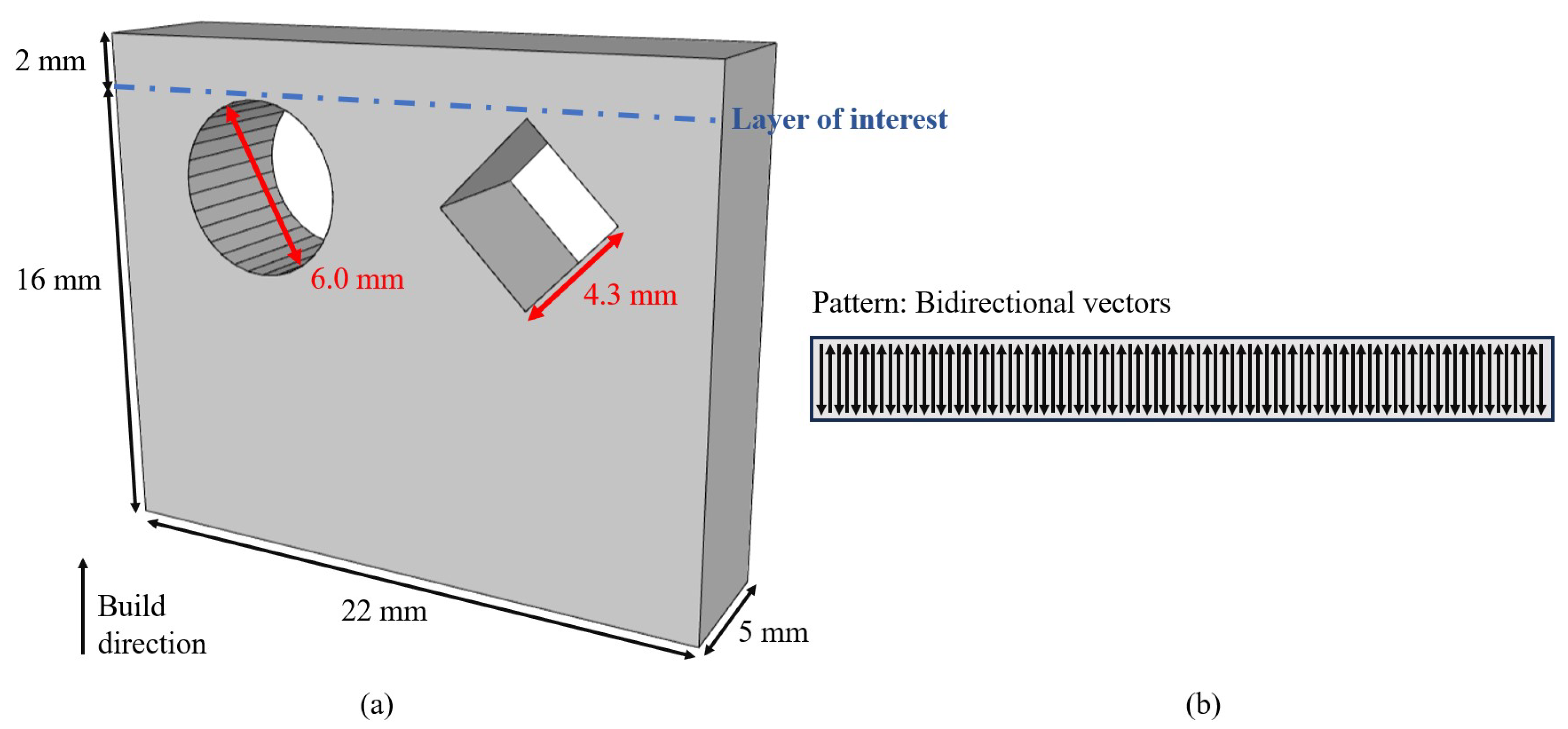
Figure 6(a) depicts a perspective view of a 3D part geometry with a 6mm diameter circular channel on the left and a diamond-shaped channel with a 4.3mm side length on the right. All the layers of the part are hatched using bidirectional vectors that are parallel to the short side as shown in Figure 6(b).

The goal of our simulations in this case study is to evaluate the benefit of providing the generalized SmartScan with probabilistic exploration in reducing the greediness of the algorithm. For this purpose, we focus on the layer highlighted in Fig. Figure 6 just above the overhangs caused by both channels, since they provide heat traps that exacerbate the greediness of the algorithm. In addition, we wish to use this case study to evaluate the benefit of the SVD-based MOR to reduce SmartScan’s computational cost without overly sacrificing its accuracy.

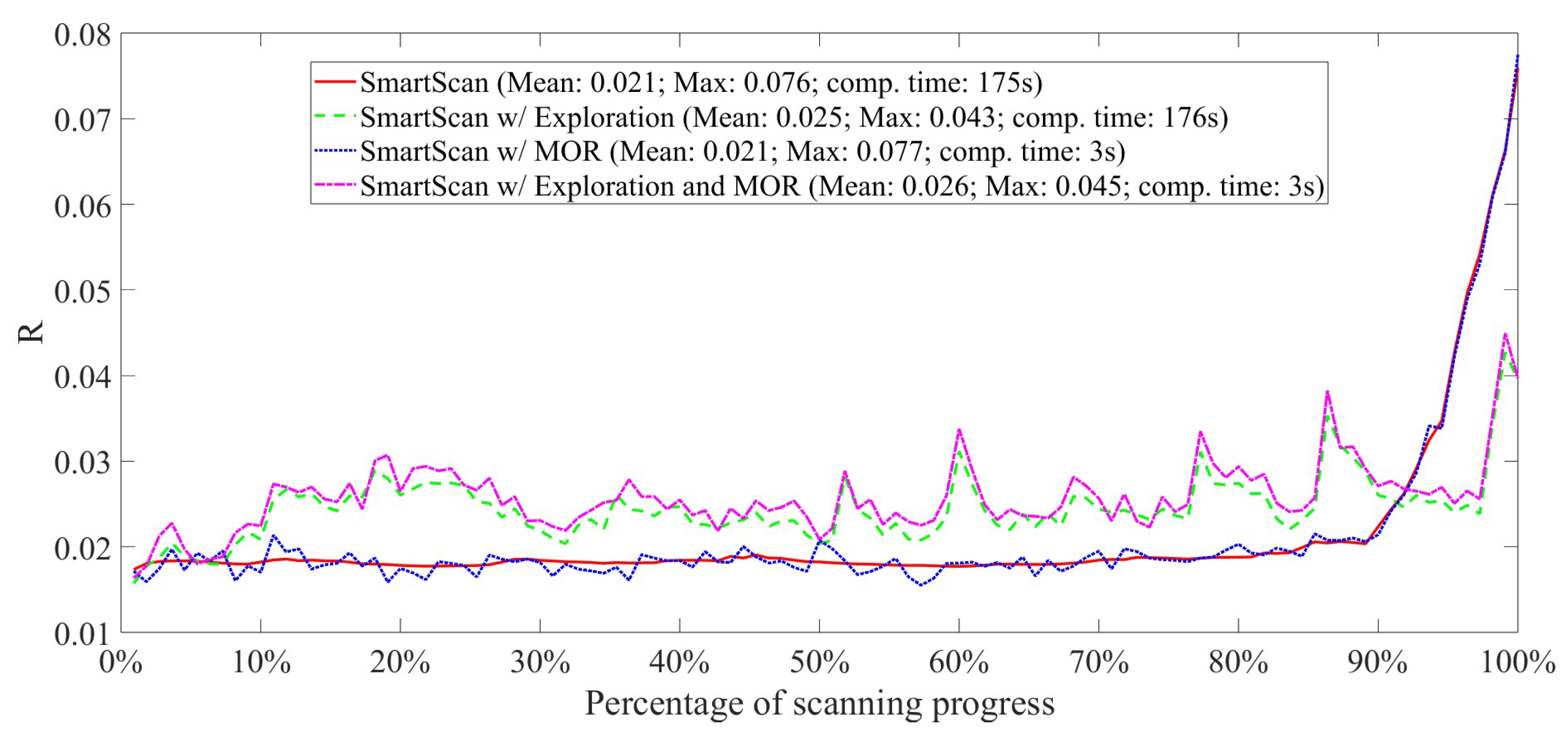
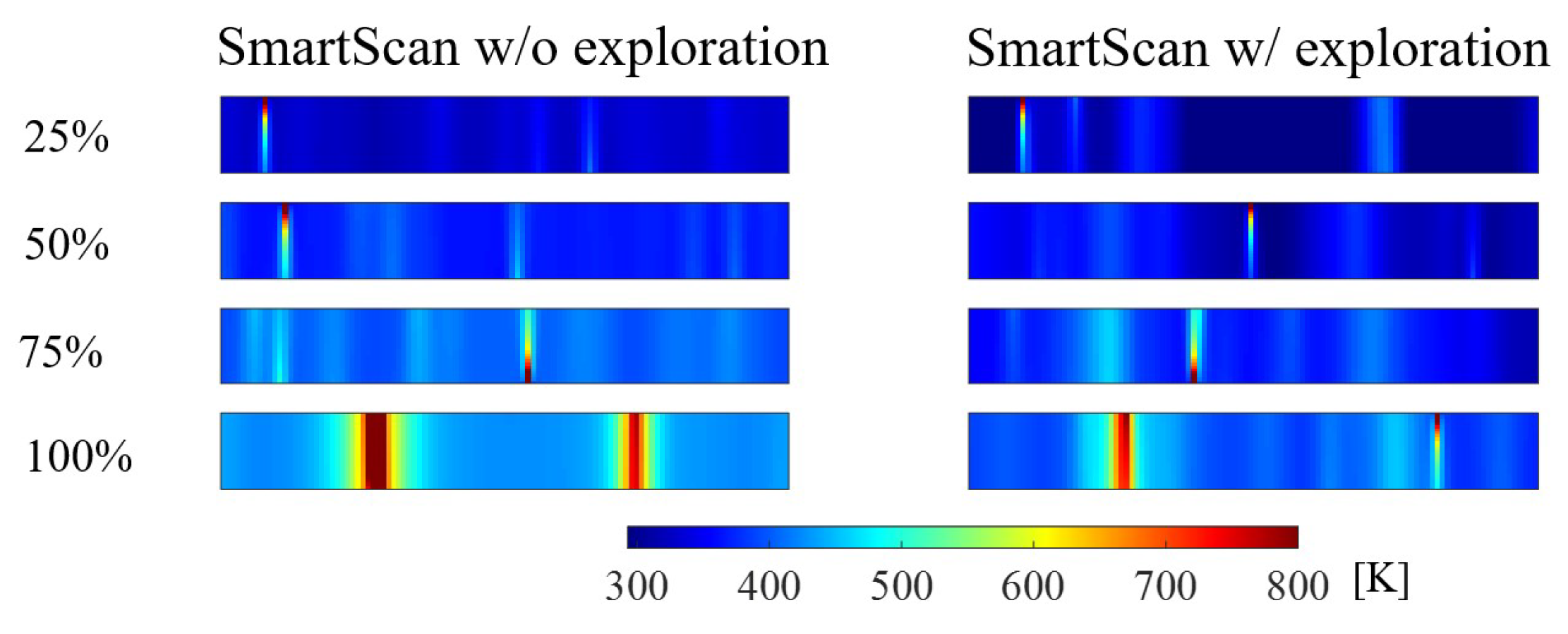
Figure 7 shows the thermal uniformity metric R as a function of scanning progress for the layer of interest. We compare four cases: (1) SmartScan (without exploration and MOR), (2) SmartScan with exploration, (3) SmartScan with MOR, and (4) SmartScan with both exploration and MOR. The addition of MOR greatly improves SmartScan’s computational efficiency by reducing the computation time for the layer of interest by 98.3%, with little or no loss in optimization performance, as indicated by the mean R value. Moreover, the addition of exploration prevents the increase in R from being drastic at the end of the print due to excessive local overheating. As a result, it reduces the maximum R value by 43.4%. This observation is confirmed by Figure 8 which shows the thermal distributions at four key stages—25%, 50%, 75%, and 100%—of the scanning progress using SmartScan with and without exploration. MOR is not applied in either case. Notice that at the end of scanning the layer, the overheating of the two overhang areas was significantly reduced due to the presence of exploration.

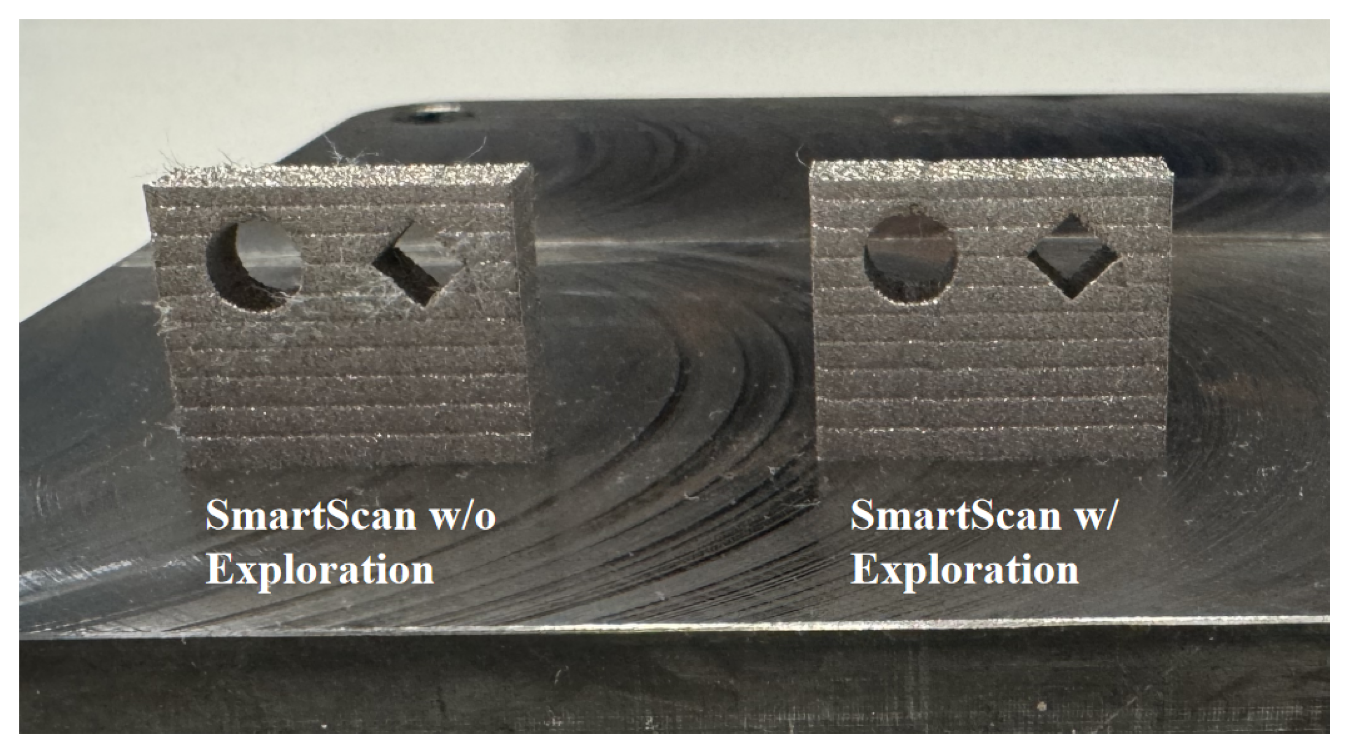
Figure 9 shows the printed part using SmartScan, without and with exploration. MOR is used in both cases to improve computational efficiency. After printing, the front side of the part was scanned using a Romer Absolute Arm 3D scanner (Hexagon, Stockholm, Sweden) model #7525SI, which has a 38

μ m

volumetric accuracy and 27

μ m

point repeatability. The resultant point clouds were transferred to MATLAB to extract information about the post-printing geometric error of the parts. The scan results of the front surface are shown in Figure 10, where the blue color represents the point cloud information obtained from the scan, and the red outline represents the nominal shape. It is evident that with the addition of exploration, the geometric accuracy of both channels has significantly improved due to less local heat accumulation around the channels. The area error refers to the cumulative value of the excessive or missing areas in the point cloud relative to the nominal shape. Without exploration, the circular and diamond-shaped channels have area errors of 1.8 mm² and 3.8 mm², respectively. With exploration, the area errors are reduced to 1.3 mm² and 1.9 mm², representing improvements of 27.8% and 50.0%, respectively. In summary, the simulation and experiment of Case Study 1 have helped validate the benefits of adding exploration and MOR to SmartScan. Therefore, every instance of SmartScan used in the following case studies will include both exploration and MOR, even if it is not explicitly stated.

3.3. Case Study 2: Cantilever Beam

Figure 11 shows a cantilever beam designed for comparing SmartScan to commonly-used heuristic sequences with regard to thermal uniformity, distortion, residual stress, and printing time. Each layer is hatched using bidirectional vectors with a 67-degree rotation of the vectors in each layer relative to those in the preceding layer [44]. SmartScan is benchmarked against two prevalent heuristic sequences: Sequential (which involves scanning the vectors consecutively from one end of the part to the other), and Alternating (which first scans every other vector consecutively, then returns to scan the remaining vectors consecutively to help distribute heat more evenly).

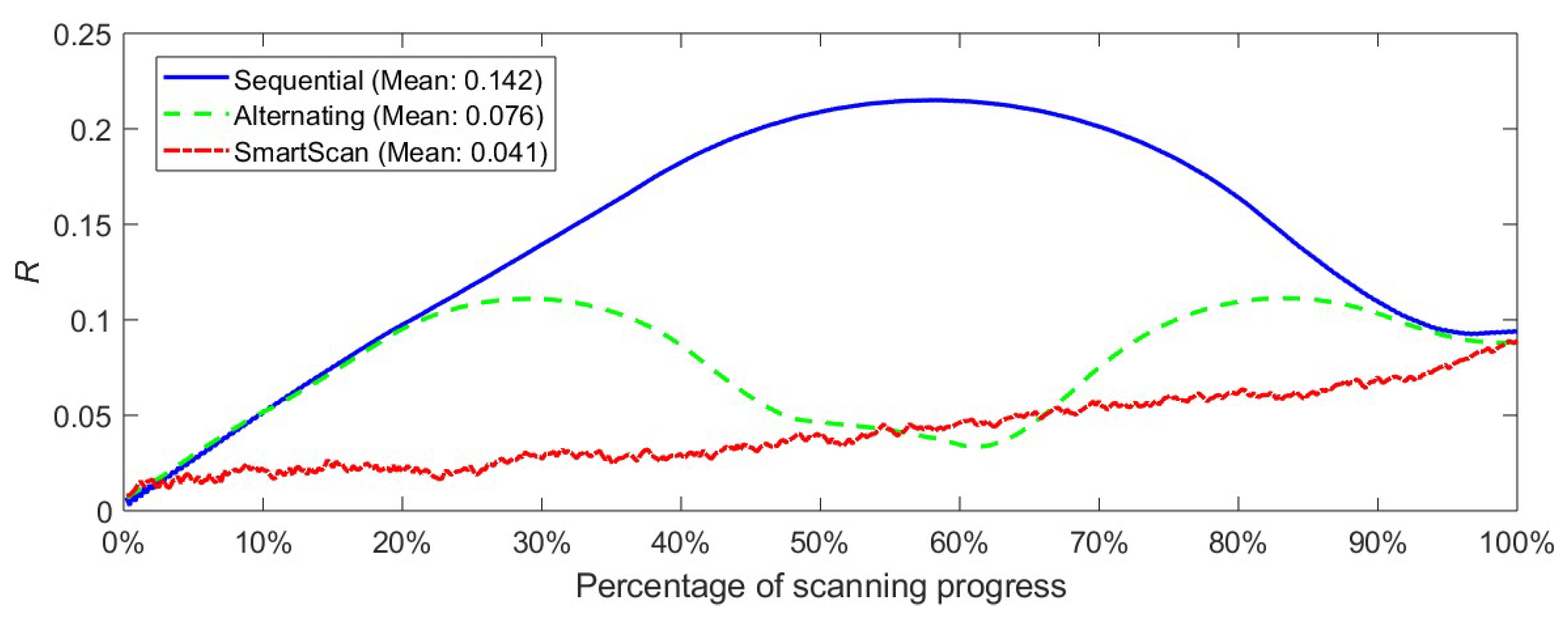
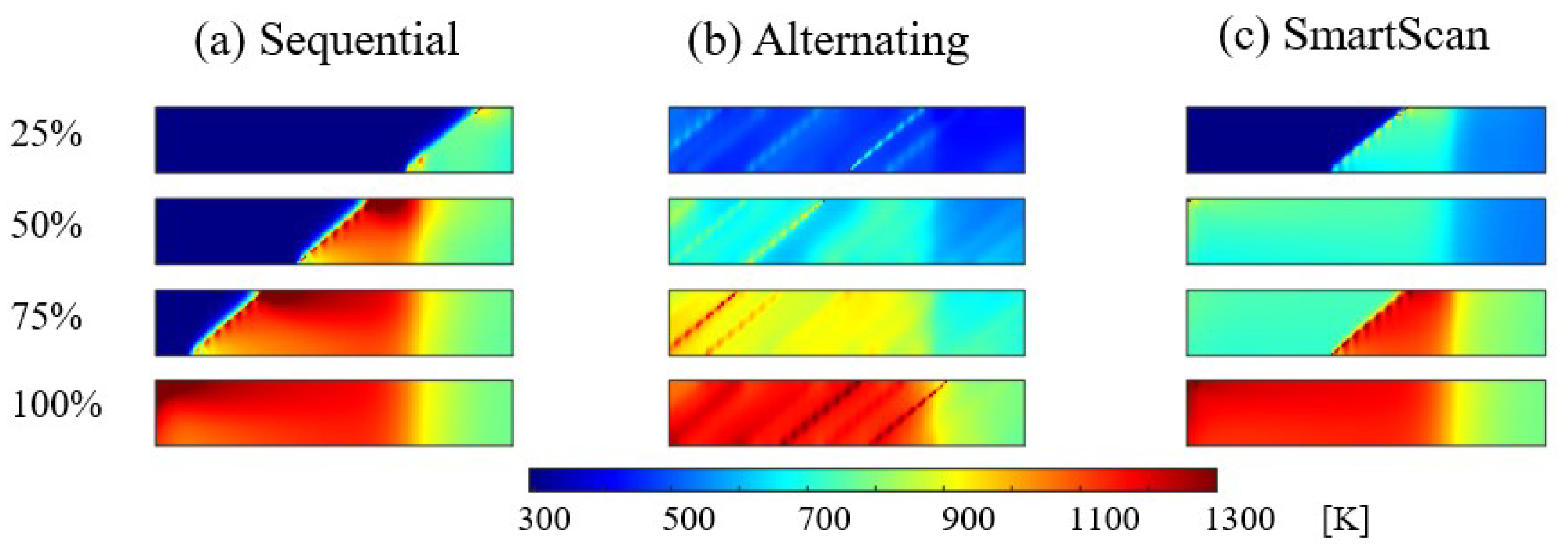
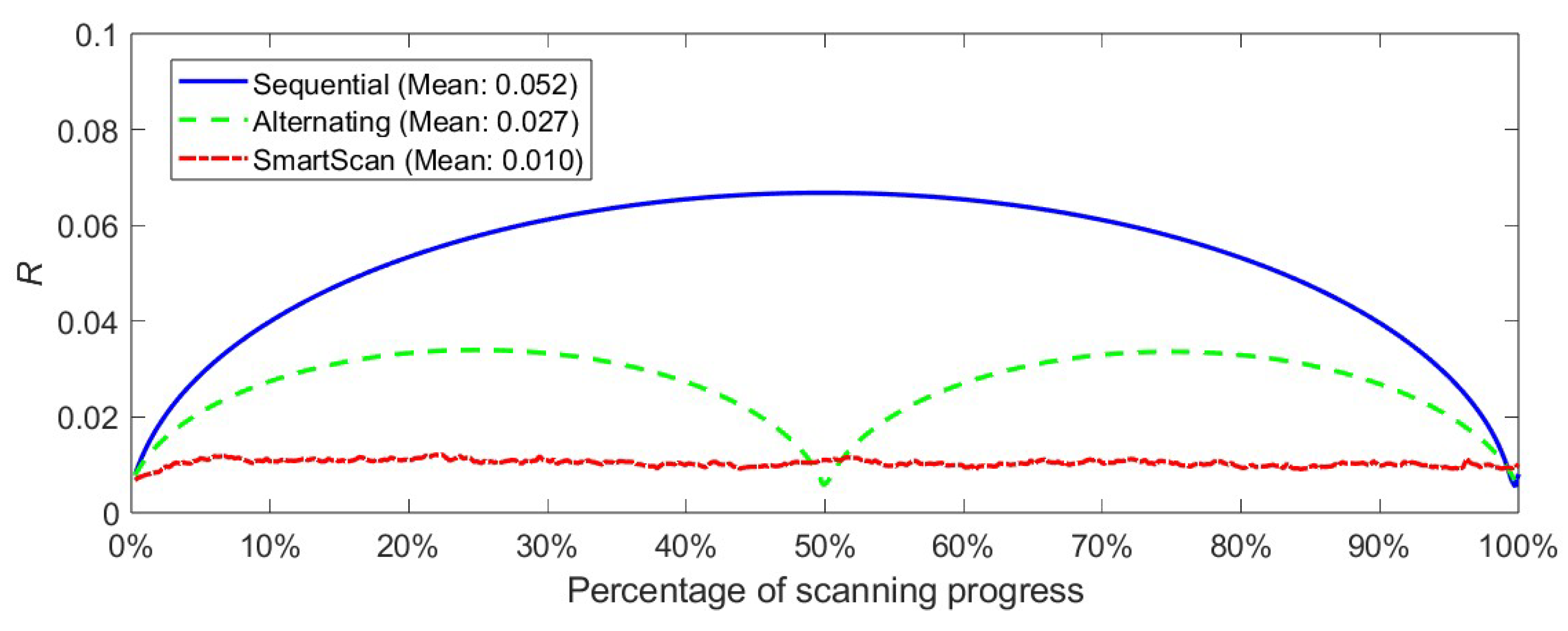
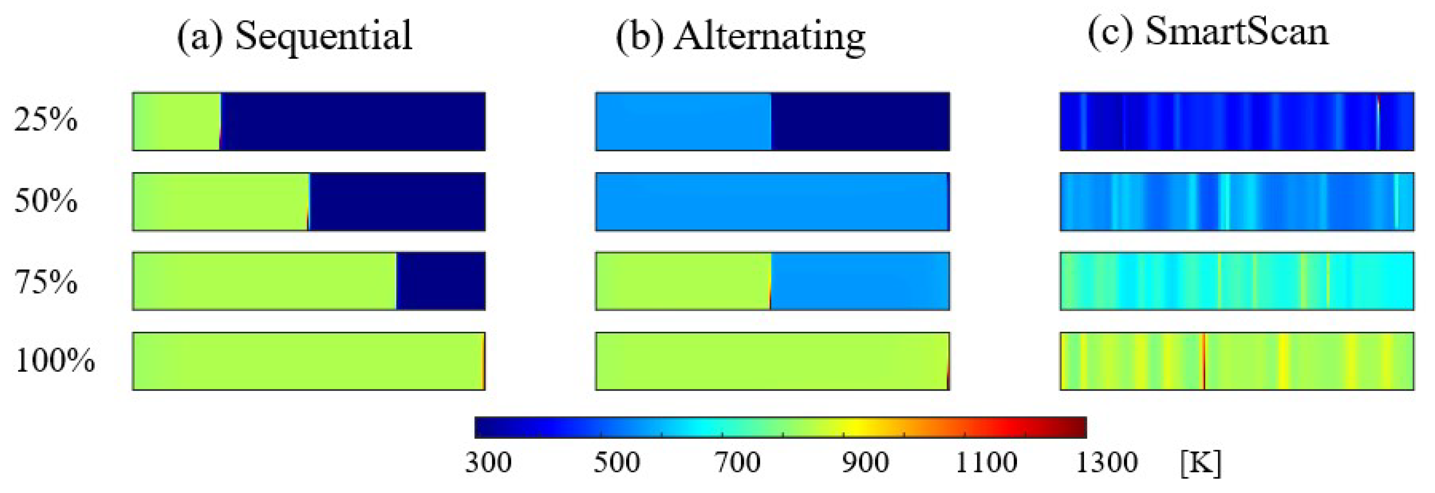
Evaluation of Thermal Uniformity: Simulations are carried out to evaluate thermal uniformity. To assist with this, two layers are investigated, namely: Layer A (the layer just above the overhangs) and Layer B (the topmost layer of the part), as shown in Figure 11. First, we investigate Layer A (the layer just above the overhangs). Figure 12 displays the temperature uniformity metric, R, (as expressed in Equation (5) relative to the scanning progress (in %). SmartScan achieves 71% and 46% lower mean R, and 64% and 25% lower maximum R than Sequential and Alternating, respectively, meaning that SmartScan delivers superior thermal uniformity compared to the benchmarks. This observation is confirmed in Figure 13 which presents the thermal distributions at four key stages—25%, 50%, 75%, and 100%—of scanning progress, with SmartScan generally exhibiting more uniform temperature distribution. Secondly, we investigate the thermal uniformity of Layer B, the topmost layer of the part. Figure 14 depicts the temperature uniformity metric, R, again as a function of scanning progression. SmartScan exhibits mean R values that are lower than those of Sequential and Alternating by 81% and 63%, respectively, and maximum R that are lower than values of Sequential and Alternating by 92% and 83%, respectively. Accordingly, the simulated temperature distributions shown in Figure 15 confirm SmartScan’s ability to provide better thermal uniformity compared to the heuristic methods.

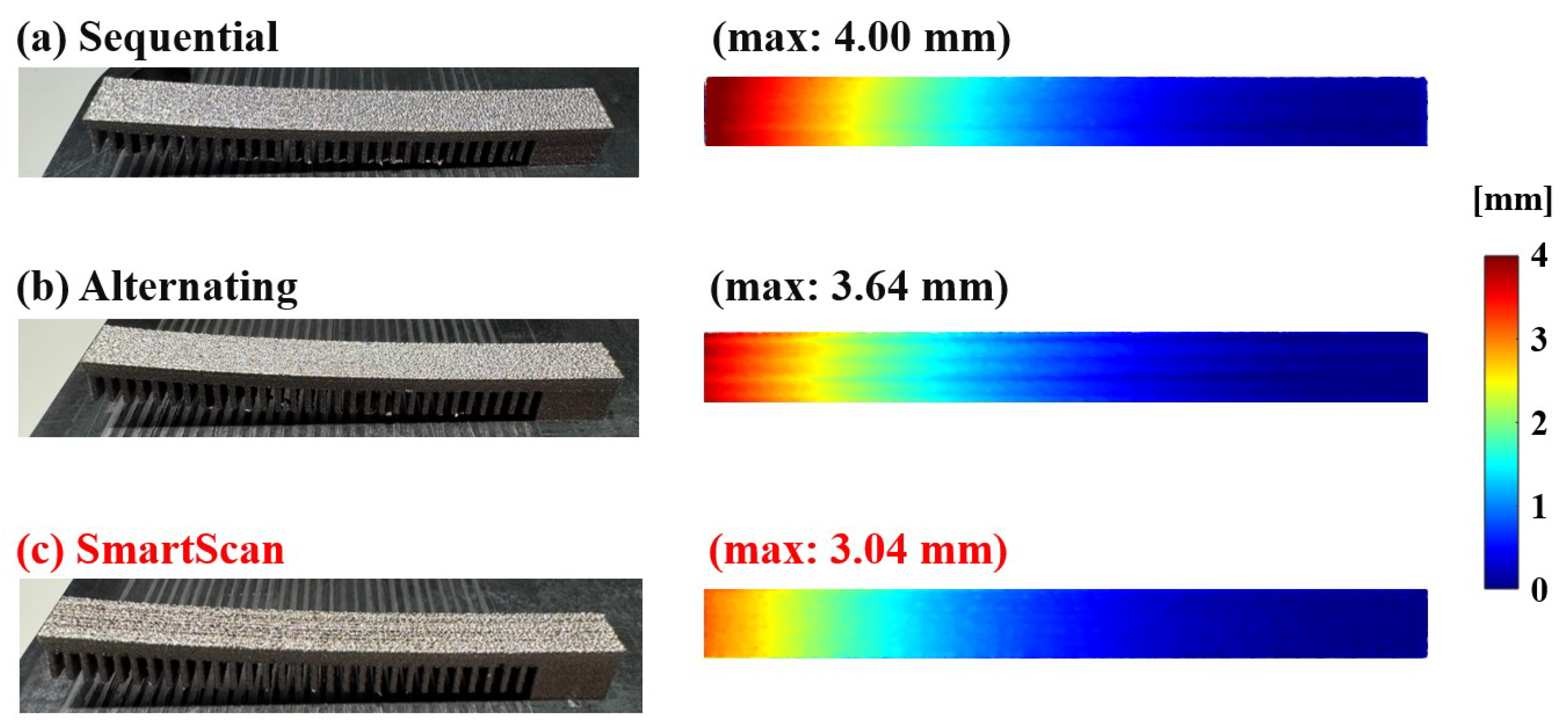
Evaluation of Distortion and Residual Stress:Figure 16 shows the printed cantilever beams using Sequential, Alternating and SmartScan strategies. They are used for experimental evaluation of the part for distortion and residual stress. To evaluate distortion, the thin support structures were sawed off the build plate using a band saw. The top surface of the part was then scanned using the Romer Absolute Arm described in Section 3.2 to extract information about the post-printing deformation of the parts. The upper surface of the part exhibited varying degrees of upward bending due to the release of some residual stress; these bending deformations were captured using point clouds. SmartScan resulted in a 24% and 16% reduction in the maximum part deflection, as well as 18% and 14% reduction in mean part deflection compared to Sequential and Alternating, respectively. While SmartScan does not completely eliminate deformation, its ability to reduce it could be very valuable in enabling parts to meet target tolerances. Moreover, it can be combined with other techniques, e.g., distortion pre-compensation [45] to further reduce deformation and improve printed part quality.

Finally, a

7 \times 7 \times 7

{mm}^{3}

specimen representing a large portion of the solid block on the right side of the cantilever beam in Figure 11 was extracted for residual stress measurements. The block does not deform significantly after sawing it off from the build plate, hence it retains a lot of the residual stress accumulated during printing. The measurements were taken in the x and y directions of a

5 \times 5 {mm}^{2}

area of the specimen (marked "C" in Figure 11). A Cu-targeted X-ray diffraction (XRD) machine (Rigaku Ultima IV XRD) was used for residual stress measurement of the specimen, and the machine’s proprietary PDLX software was used for data analysis. The machine was operated at

40 k V

and

40 m A

for measurements. The

{sin}^{2} ψ

method was applied for the stress analysis with various tilt angles (

- 30^{\circ}

- 25^{\circ}

- 20^{\circ}

- 15^{\circ}

- 10^{\circ}

0^{\circ}

) for two series of samples, and the elastic modulus was kept constant at

190 GPa

while the Poisson ratio was taken as 0.265 for each sample.

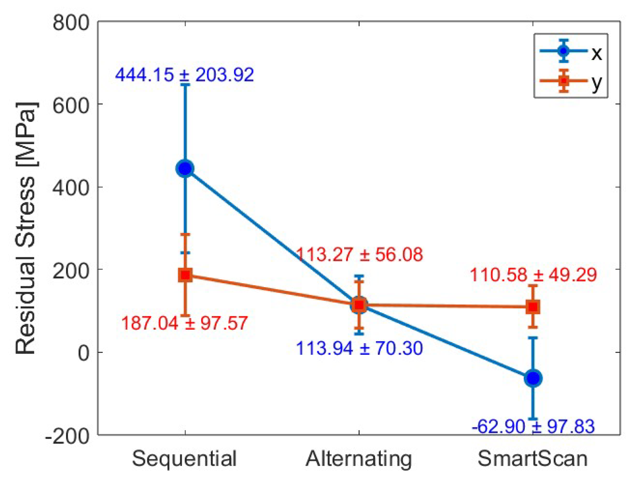
Figure 17 summarizes the results of the residual stress measurements using XRD. SmartScan resulted in a 86% and 45% reduction of the mean value of the x-component of residual stress, and a 41%, and 2% reduction in the y-direction of residual stress (mean value) compared to Sequential and Alternating, respectively. The large reductions in residual stress provided by SmartScan could be beneficial in practice because it decreases the risk of print failures directly caused by excessive stress during the printing process, before post-process stress relief. With lower as-built residual stress, the duration of the heat treatment process could also be shortened, which decreases the energy consumption of the post processing step [46].

Evaluation of Printing Time and Computational Cost:Table 2 shows the recorded print time for each sample obtained during the printing experiments. According to the data for the vector pattern, SmartScan caused a 5% increase in print time compared to both Sequential and Alternating due to the increased jump time as the laser moves from one vector to the other. This suggests that the use of SmartScan does not result in substantial increases in print time when compared to heuristic sequences. This can be credited to the laser’s jump speed being significantly faster than its scan speed.

In addition, the computation cost is also an important consideration for SmartScan, as it affects the practicality of the method. In the experiments reported above, SmartScan optimized each layer of the part within 10 seconds using an AMD Ryzen 9 7945HX processor, 32.0 GB RAM and NVIDIA GeForce RTX 4070 Laptop GPU. Most of the computation is based on GPU and the computational time of SmartScan is reasonable, as it is close to the interlayer powder recoating time of LPBF. Its computational time can be further reduced by leveraging parallel computing and code optimization.

3.4. Case Study 3: Complex 3D Part

So far, the geometries used for evaluating SmartScan have been fairly simple. However, in practice, LPBF is often used to print complex geometries. One approach to enable the use of SmartScan for printing complex geometries is to embed it as a plug-in to commercial slicers which already have the capability to process complex geometries. The idea is as follows. A complex geometry is sliced using a commercial slicer resulting in a scan pattern with repeating features (e.g., vectors, islands, or fragments) for each layer. This information is fed into the SmartScan plug-in along with the material properties and other key parameters needed by the algorithm. The SmartScan plug-in processes and then outputs the optimal sequence of the features for each layer, which is compiled into an appropriate output file format that can be sent to an LPBF machine to print the part.

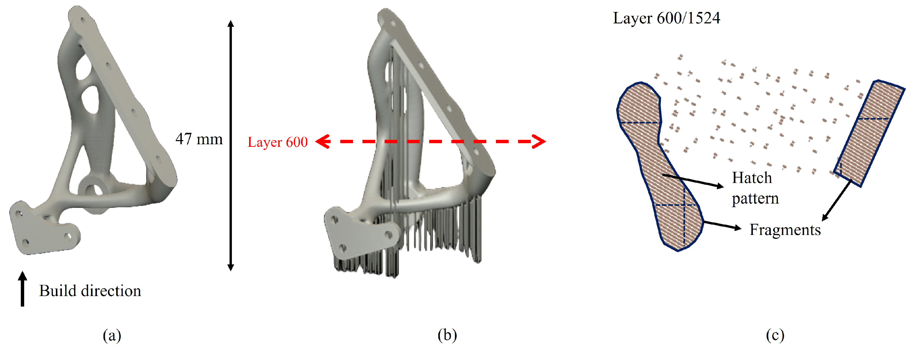
To test this idea, in partnership with Ulendo Technologies, Inc. (Ann Arbor, MI) a SmartScan plug-in was created for a commercial slicing software, Dyndrite LPBF Pro, developed by Dyndrite Corporation (Seattle, WA). Figure 18(a) shows a complex bracket part [47] that was used to test the performance of the SmartScan plug-in. The slicer added supports as shown in Figure 18(b). Then it sliced the part such that the infill portion of each layer consisted of features called fragments, that are filled with a hatch pattern (see Figure 18(c)). The SmartScan plug-in reordered the fragments in each layer based on the algorithm described in Section 2, then returned the optimal sequence (i.e., the re-ordered fragments) to the slicing software. The software then outputted the result as a common layer interface (CLI) file that was used to print the part on the PANDA 11 LPBF machine. The SmartScan print was benchmarked against the same part printed using a scan sequence generation method, called sort_by_distance, provided as a default option in Dyndrite LPBF Pro. The computational cost to optimize the part using the SmartScan plug-in was approximately 16 minutes on the same PC with a GPU used in Sec. 3.3, which is an average of 1.2 seconds per layer. The part generated using the SmartScan plug-in took 308 minutes to print, compared to 304 minutes using the default sequence. These further confirm that the computational cost and printing time using SmartScan are reasonable even for complex 3D shapes.

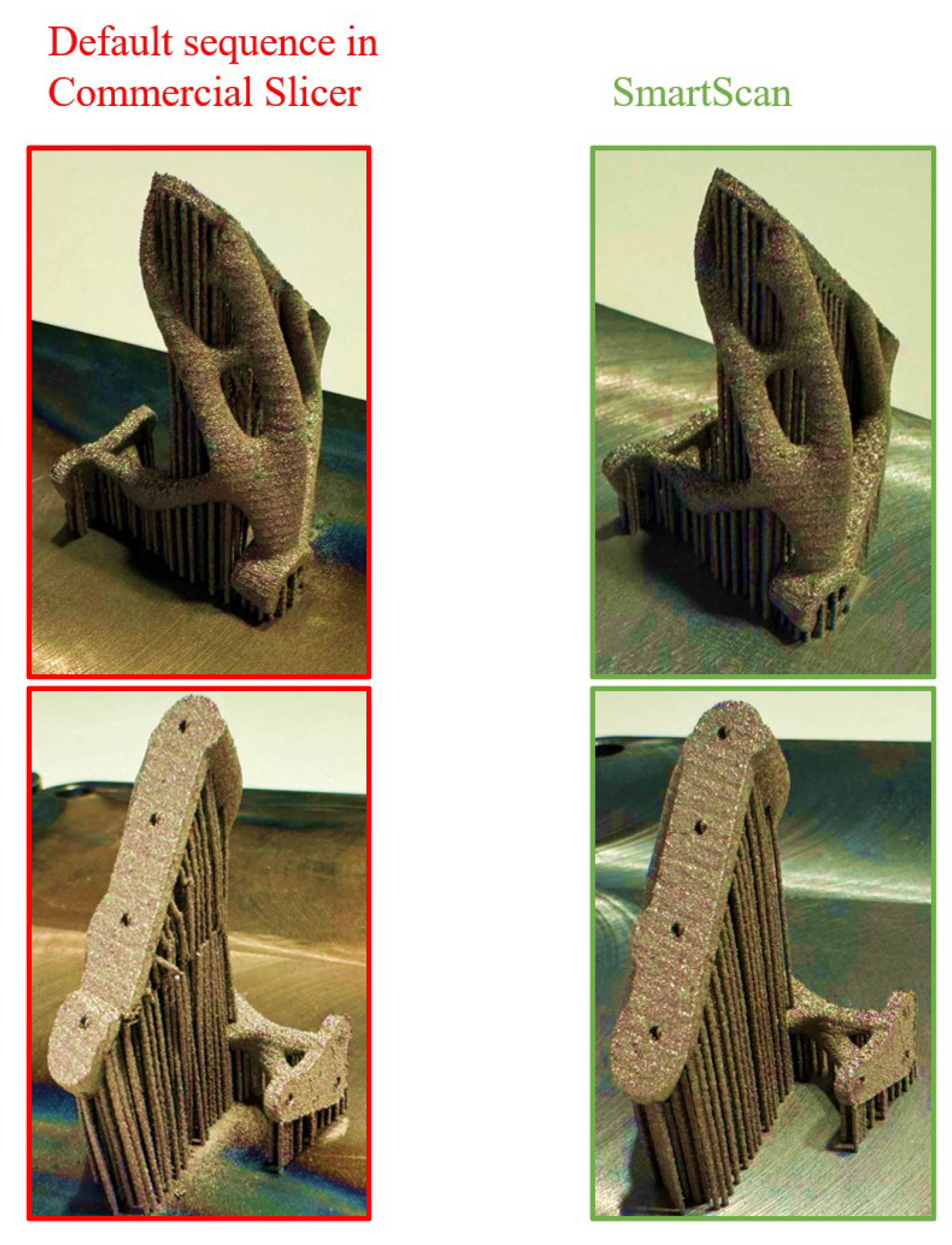
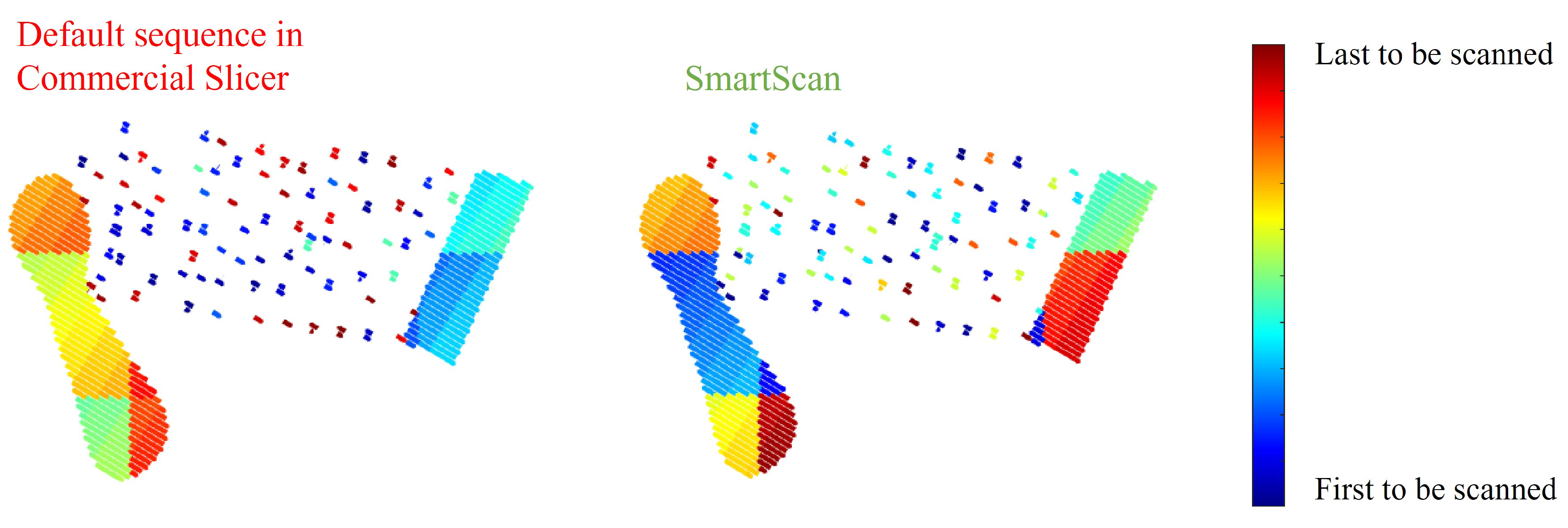
Figure 19 shows a comparison of the parts printed using the default sequence and the SmartScan plug-in. Notice that with the default sequence, the print fails because some of the supports break and a portion of the part collapses. However, with SmartScan, the part prints successfully. The reason for this difference can be seen in Figure 20, which compares the scan sequences at layer 600 (near the defect). Notice that the default sequence scans the fragments that are in close proximity to each other consecutively, thus increasing the potential for excessive heat and stress build up. Conversely, SmartScan avoids scanning close islands consecutively, thus reducing the potential for heat and stress build up.

4. Conclusions and Future Work

In this paper, we have presented a generalized SmartScan methodology that uses thermal models and control-theory-based optimization of scan sequence to address critical challenges of thermal inhomogeneity, residual stress and distortion in parts made using LPBF. It builds on our prior work on SmartScan [31,34] by: (1) expanding the thermal model and optimization approach from a single layer to multiple layers; (2) enabling SmartScan to process shapes with arbitrary contours and infill patterns within each layer; (3) providing SmartScan with probabilistic exploration to make it less myopic in its optimization; and (4) furnishing SmartScan with SVD-based MOR to enhance its computational efficiency. The net result of these contributions is that the generalized SmartScan is capable of optimizing scan sequence for arbitrary 3D geometries.

We have shown the benefits of generalized SmartScan in both simulations and experiments on a variety of test artifacts leading to the following conclusions:

The incorporation of probabilistic exploration enables SmartScan to be less greedy, allowing it to process 3D geometries with overhangs and heat traps without excessive local overheating. This capability was shown to yield up to 50% improvement in geometric accuracy of a test artifact compared to a version of SmartScan without probabilistic exploration.
The addition of SVD-based MOR to SmartScan improved its computational efficiency significantly with little or no losses its accuracy. In a case study, this contribution resulted in up to 58 times reduction in computation time compared to a version of SmartScan without MOR.
Similar to the results seen in 2D case studies in our prior work [31,34], SmartScan demonstrated significant reductions in thermal inhomogeneity, residual stress and deformation compared to commonly-used heuristic scan sequences, with minimal increases in printing time. These were demonstrated on a cantilever beam case study where reductions of up to 92% in temperature inhomogeneity, 86% in residual stress, and 24% in maximum deflection were achieved, with only 5% increase in printing time.
The computational cost of SmartScan is very reasonable for practical applications. It generally optimizes each layer in less than the typical interlayer powder recoating time of LPBF, which makes it practical for offline or online implementation.
SmartScan can readily be deployed in practice for processing complex 3D parts by, for example, integrating it as a plug-in to commercial slicing software. This capability was demonstrated using a case study of a complex 3D bracket where the SmartScan plug-in to a commercial slicer was used to produce a successful print while the default scanning sequence of the commercial slicer resulted in a failed print.

In future research, we plan to investigate the impacts of SmartScan on microstructure, porosity, surface roughness and other properties of parts printed using LPBF that are influenced (directly or indirectly) by scan sequence. We also plan on testing SmartScan on a variety of materials beyond 316L stainless steel to evaluate any effects of material type on the results of the algorithm. Another interesting avenue for further research we plan to pursue is to incorporate thermomechanical models and objective functions into SmartScan, as opposed to the purely thermal models and objectives used in this work and our prior work. This may yield better results since some of the phenomena, like residual stress and distortion, addressed by SmartScan are thermomechanical rather than purely thermal in nature.

Author Contributions

Acknowledgments

This project was funded in part by a Michigan Translational Research and Commercialization (MTRAC) grant provided by the Michigan Economic Development Corporation. The authors thank Mr. Samuel Thompson, Mr. Oguz Esen and Mr. Dilip Raj of Ulendo Technologies, Inc., as well as Dr. Steve Walton and Mr. Dahlon Lyles of Dyndrite Corporation, for their assistance in developing the SmartScan plug-in used in this paper.

Conflicts of Interest

The authors declare the following financial interests/personal relationships which may be considered as potential competing interests: The Regents of the University of Michigan have applied for patents related to SmartScan and licensed SmartScan to Ulendo Technologies, Inc., a company founded by one of the authors of this paper.

Abbreviations

Notation	Definition	Unit
AM	Additive manufacturing
CLI	Common layer interface
LHI	Least heat influence
LPBF	Laser powder bed fusion
MOR	Model order reduction
SVD	Singular value decomposition
TH	Time-homogenization
XRD	X-ray diffraction
$A$	State matrix
$A_{f}$	Feature-level state matrix of fth feature
$\tilde{A}$	Reduced state matrix
$B$	Input matrix
$\tilde{B}$	Reduced input matrix
$C$	Output matrix
$\tilde{C}$	Reduced output matrix
$C_{p}$	Specific heat capacity	$J \cdot {kg}^{- 1} \cdot K^{- 1}$
$I$	Identity matrix
$N_{f}$	The number of time steps to trace feature f
R	Temperature uniformity metric
$SF$	The internal dynamics for all candidates
T	Temperature	K
$T$	Temperature state vector
$\tilde{T}$	Reduced state
$T_{a}$	Ambient temperature	K
$T_{avg}$	Mean temperature	K
$T_{b}$	Temperature of the substrate (base plate)	K
$T_{m}$	Melting point of the material	K
$b_{f}$	Feature-level input vector of fth feature
$f$	Feature index
$g_{f}$	The set of all time steps associated with feature f
h	Convection coefficient	$W \cdot m^{- 2} \cdot K^{- 1}$
i	Spatial index of the element in the x-axis
j	Spatial index of the element in the y-axis
k	Spatial index of each layer
$k_{t}$	Conductivity	$W \cdot m^{- 1} \cdot K^{- 1}$
$k^{*}$	Spatial index of the FDM bottom layer
l	Temporal index
Notation	Definition	Unit
$n_{F}$	The number of features in a layer
$n_{k}$	Number of elements in layer k
$n_{e}$	Number of elements in full-scale model
$n_{r}$	Number of elements in reduced model
$p$	Probability
t	Time	s
$Δ t$	Time step	s
$u$	Power per unit volume	$W \cdot m^{- 3}$
x	Spatial coordinate in the x-axis
$Δ x$	Dimensions of each element in the x-axis	m
y	Spatial coordinate in the y-axis
$Δ y$	Dimensions of each element in the y-axis	m
z	Spatial coordinate in the z-axis
$Δ z$	Dimensions of each element in the z-axis	m
$1$	All-ones column vector
$0$	Null matrix
$Φ$	Projection matrix
$α$	Diffusivity	$m^{2} \cdot s^{- 1}$
$β$	Pre-computed scalar
$γ$	Pre-computed vector
$δ$	Pre-computed matrix
$η$	Absorptance
$λ$	Selection metric
$μ$	Mean of Gaussian distribution
$σ$	Standard deviation of Gaussian distribution
$ρ$	Density	$kg \cdot m^{- 3}$

Appendix A

Appendix A.1. Validation of the Effectiveness of the Chosen Values for k *

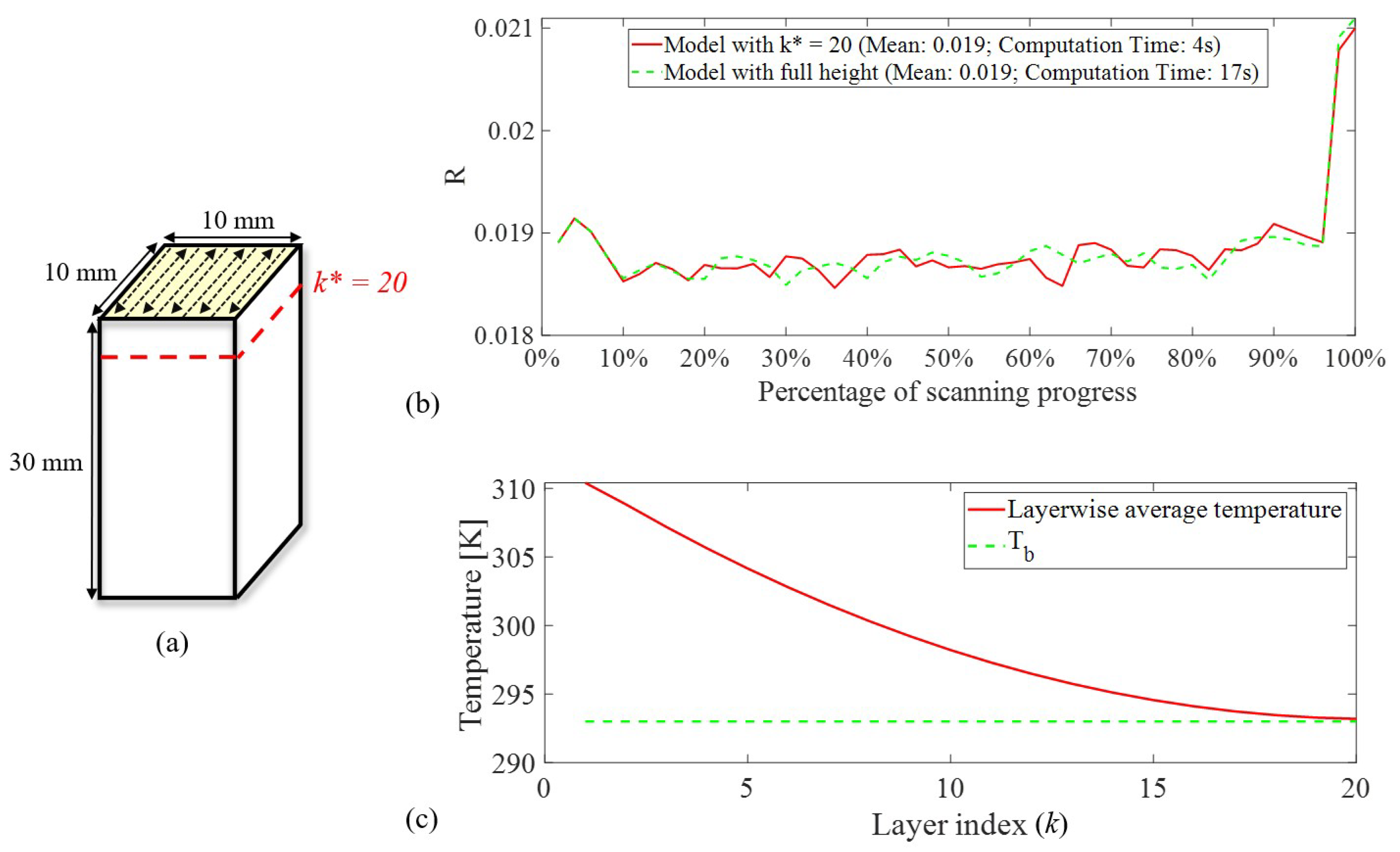
As shown in Figure A1(a), a simulation is conducted for the top layer of this rectangular prism with a small cross-sectional area of 100 mm² and a height of 30 mm. The small cross sectional area facilitates heat accumulation. The material used in the simulation was AISI 316L and the simulation parameters are as reported in Table 1. The aim of the simulation is to demonstrate that a SmartScan solution with

k^{*} = 20

yields sufficiently accurate results when benchmarked against SmartScan solution that uses the full height of the model. Figure A1(b) shows the thermal uniformity metric R calculated using the full model and the reduced model with

k^{*} = 20

for the topmost layer of the part, that experiences the most heat accumulation. The R values for both cases are nearly identical, indicating that the use of

k^{*} = 20

in all the simulations performed in this paper is sufficiently accurate. Figure A1(c) confirms that when

k^{*}

is chosen to be 20, the average temperature of the

k^{*} = 20

layer is nearly equal to

T_{b}

at the moment when the topmost layer (

k = 1)

is fully scanned by the laser.

Figure A1. (a) A model used to validate the effectiveness of the

k^{*}

selection; (b) A comparison of optimization results between using the reduced model and the full-scale model; (c) The relationship between the average temperature of each layer (k) and

T_{b}

just after the topmost layer (

k = 1

) is fully scanned.

Figure A1. (a) A model used to validate the effectiveness of the

k^{*}

selection; (b) A comparison of optimization results between using the reduced model and the full-scale model; (c) The relationship between the average temperature of each layer (k) and

T_{b}

just after the topmost layer (

k = 1

) is fully scanned.

Appendix A.2. Construction of the System Matrix Included in Equation (uid11)

The convergence of prediction outcomes is critically dependent on both cell size and time increments. In our calculations, the edge length of cells (

Δ x

Δ y

and

Δ z

) and the time increment

Δ t

were determined in accordance with the recommendations provided by Yang et al. [48].

The heat transfer equations presented in Equation (1) were solved using the finite difference method, as described in Equation (2). For the purpose of updating the thermal field at each time step as prescribed by Equation (3) in state-space representation form, it is necessary to analyze the surrounding conditions of each cell. This analysis is grounded in diverse heat transfer characteristics to facilitate the precise construction of matrix

A

. As shown in Figure A2, the target cell (marked in orange) is connected to two cells along the x-axis, two cells along the y-axis, and one cell along the z-axis. Additionally, it experiences convection due to its upper surface being exposed to the surrounding space. Thus, over a time period

Δ t

, its temperature can be predicted as follows:

\begin{matrix} T (i, j, k, l + 1) = α \frac{Δ t}{{(Δ x)}^{2}} \{T (i + 1, j, k, l) + T (i - 1, j, k, l)\} \\ + α \frac{Δ t}{{(Δ y)}^{2}} \{T (i, j + 1, k, l) + T (i, j - 1, k, l)\} + α \frac{Δ t}{{(Δ z)}^{2}} \{T (i, j, k - 1, l)\} \\ + [1 - 2 α \frac{Δ t}{{(Δ x)}^{2}} - 2 α \frac{Δ t}{{(Δ y)}^{2}} - α \frac{Δ t}{{(Δ z)}^{2}}] T (i, j, k, l) \\ - \frac{Δ t}{Δ z} (\frac{h}{ρ C_{p}}) [T (i, j, k, l) - T_{a}] \end{matrix}

(A1)

where

ρ

represents density, and

C_{p}

represents specific heat capacity. The above equation can be expressed in vector form:

\begin{matrix} T (i, j, k, l + 1) = \\ [\begin{matrix} α_{x} & α_{x} & α_{y} & α_{y} & 0 & α_{z} & 1 - 2 α_{x} - 2 α_{y} - α_{z} - h_{z} & h_{z} & 0 \end{matrix}] [\begin{matrix} T (i + 1, j, k, l) \\ T (i - 1, j, k, l) \\ T (i, j + 1, k, l) \\ T (i, j - 1, k, l) \\ T (i, j, k + 1, l) \\ T (i, j, k - 1, l) \\ T (i, j, k, l) \\ T_{a} \\ T_{b} \end{matrix}] \\ α_{x} = α \frac{Δ t}{{(Δ x)}^{2}}; α_{y} = α \frac{Δ t}{{(Δ y)}^{2}}; α_{z} = α \frac{Δ t}{{(Δ z)}^{2}}; h_{z} = \frac{Δ t}{Δ z} (\frac{h}{ρ C_{p}}) \end{matrix}

(A2)

Figure A2. Finite difference method used in heat transfer.

To construct the system’s matrix

A

, we assembled the corresponding rows obtained from the analysis of each cell as instructed by the example in Equation (A2).

Table A1. Finite difference approximations to the spatial derivatives of Equation (1) [49] for interior and boundary nodes in every direction, to be substituted as necessary into Equation (1) for each node based on its boundary classification.

	Left boundary	Interior	Right boundary
$\frac{\partial^{2} T}{\partial x^{2}} \|_{i, j, k}$	$\frac{- T_{(i + 2), j, k} + 8 T_{(i + 1), j, k} - 7 T_{i, j, k}}{2 Δ x^{2}}$	$\frac{T_{(i - 1), j, k} - 2 T_{i, j, k} + T_{(i + 1), j, k}}{Δ x^{2}}$	$\frac{- T_{(i - 2), j, k} + 8 T_{(i - 1), j, k} - 7 T_{i, j, k}}{2 Δ x^{2}}$
$\frac{\partial^{2} T}{\partial y^{2}} \|_{i, j, k}$	$\frac{- T_{i, (j + 2), k} + 8 T_{i, (j + 1), k} - 7 T_{i, j, k}}{2 Δ y^{2}}$	$\frac{T_{i, (j - 1), k} - 2 T_{i, j, k} + T_{i, (j + 1), k}}{Δ y^{2}}$	$\frac{- T_{i, (j - 2), k} + 8 T_{i, (j - 1), k} - 7 T_{i, j, k}}{2 Δ y^{2}}$
$\frac{\partial^{2} T}{\partial z^{2}} \|_{i, j, k}$	$\frac{- 2 T_{i, j, k} + T_{i, j, (k + 1)}}{Δ z^{2}} + \frac{1}{Δ z^{2}} T_{b}$	$\frac{T_{i, j, (k - 1)} - 2 T_{i, j, k} + T_{i, j, (k + 1)}}{Δ z^{2}}$	$\frac{- T_{i, j, (k - 2)} + 8 T_{i, j, (k - 1)} - (7 + 6 \frac{h Δ z}{k}) T_{i, j, k}}{2 Δ z^{2}} + \frac{3 h}{k Δ z} T_{a}$

Also, the temperature of the cells exposed to the heat source was dynamically updated in accordance with the movement of the heat source using:

\begin{matrix} T (i, j, k, l + 1) = T (i, j, k, l) + \frac{Δ t η}{ρ \cdot Δ x Δ y Δ z \cdot C_{p}} * u (i, j, k, l) \end{matrix}

(A3)

where

η

represents the laser absorption efficiency, and

u (i, j, k, l)

denotes the laser power received at point

(i, j, k)

at time l.

References

Chowdhury, S.; Yadaiah, N.; Prakash, C.; Ramakrishna, S.; Dixit, S.; Gupta, L.R.; Buddhi, D. Laser powder bed fusion: a state-of-the-art review of the technology, materials, properties & defects, and numerical modelling. Journal of Materials Research and Technology 2022, 20, 2109–2172. [Google Scholar]
Kotadia, H.; Gibbons, G.; Das, A.; Howes, P. A review of Laser Powder Bed Fusion Additive Manufacturing of aluminium alloys: Microstructure and properties. Additive Manufacturing 2021, 46, 102155. [Google Scholar] [CrossRef]
Parry, L.; Ashcroft, I.; Wildman, R. Understanding the effect of laser scan strategy on residual stress in selective laser melting through thermo-mechanical simulation. Additive Manufacturing 2016, 12, 1–15. [Google Scholar] [CrossRef]
Dong, G.; Wong, J.C.; Lestandi, L.; Mikula, J.; Vastola, G.; Jhon, M.H.; Dao, M.H.; Kizhakkinan, U.; Ford, C.S.; Rosen, D.W. A part-scale, feature-based surrogate model for residual stresses in the laser powder bed fusion process. Journal of Materials Processing Technology 2022, 304, 117541. [Google Scholar] [CrossRef]
Chen, Q.; Taylor, H.; Takezawa, A.; Liang, X.; Jimenez, X.; Wicker, R.; To, A.C. Island scanning pattern optimization for residual deformation mitigation in laser powder bed fusion via sequential inherent strain method and sensitivity analysis. Additive Manufacturing 2021, 46, 102116. [Google Scholar] [CrossRef]
Cao, S.; Zou, Y.; Lim, C.V.S.; Wu, X. Review of laser powder bed fusion (LPBF) fabricated Ti-6Al-4V: process, post-process treatment, microstructure, and property. Light: Advanced Manufacturing 2021, 2, 1. [Google Scholar] [CrossRef]
Guo, C.; Li, S.; Shi, S.; Li, X.; Hu, X.; Zhu, Q.; Ward, R.M. Effect of processing parameters on surface roughness, porosity and cracking of as-built IN738LC parts fabricated by laser powder bed fusion. Journal of Materials Processing Technology 2020, 285, 116788. [Google Scholar] [CrossRef]
Khan, H.M.; Karabulut, Y.; Kitay, O.; Kaynak, Y.; Jawahir, I.S. Influence of the post-processing operations on surface integrity of metal components produced by laser powder bed fusion additive manufacturing: a review. Machining Science and Technology 2021, 25, 118–176. [Google Scholar] [CrossRef]
Kumar, V.P.; Jebaraj, A.V. Comprehensive review on residual stress control strategies in laser-based powder bed fusion process– Challenges and opportunities. Lasers in Manufacturing and Materials Processing 2023, 10, 400–442. [Google Scholar] [CrossRef]
Reiff, C.; Bubeck, W.; Krawczyk, D.; Steeb, M.; Lechler, A.; Verl, A. Learning Feedforward Control for Laser Powder Bed Fusion. Procedia CIRP 2021, 96, 127–132. [Google Scholar] [CrossRef]
Cao, Y.; Moumni, Z.; Zhu, J.; Gu, X.; Zhang, Y.; Zhai, X.; Zhang, W. Effect of scanning speed on fatigue behavior of 316L stainless steel fabricated by laser powder bed fusion. Journal of Materials Processing Technology 2023, 319, 118043. [Google Scholar] [CrossRef]
Riensche, A.; Bevans, B.D.; Smoqi, Z.; Yavari, R.; Krishnan, A.; Gilligan, J.; Piercy, N.; Cole, K.; Rao, P. Feedforward control of thermal history in laser powder bed fusion: Toward physics-based optimization of processing parameters. Materials & Design 2022, 224, 111351. [Google Scholar] [CrossRef]
Wang, R.; Standfield, B.; Dou, C.; Law, A.C.; Kong, Z.J. Real-time process monitoring and closed-loop control on laser power via a customized laser powder bed fusion platform. Additive Manufacturing 2023, 66, 103449. [Google Scholar] [CrossRef]
Zhang, J.; Patel, S.; Liu, Z.; Lyu, T.; Wang, Y.; Hua, Y.; Wang, W.; Hattrick-Simpers, J.; Vlasea, M.; Zou, Y. A data-driven framework to improve the wear resistance of a low-alloy steel fabricated by laser powder bed fusion. Journal of Manufacturing Processes 2024, 115, 56–67. [Google Scholar] [CrossRef]
Hu, Z.; Gao, S.; Tai, J.; Qu, S.; Ding, J.; Song, X.; Fan, Z. Columnar grain width control for SS316L via hatch spacing manipulation in laser powder bed fusion. Materials Research Letters 2023, 11, 231–238. [Google Scholar] [CrossRef]
Zhang, Z.; Wang, S.; Liu, H.; Wang, L.; Xiao, X. Effects of hatch distance on the microstructure and mechanical anisotropy of 316 L stainless steel fabricated by laser powder bed fusion. Journal of Materials Engineering and Performance 2023, 32, 4757–4767. [Google Scholar] [CrossRef]
Boissier, M.; Allaire, G.; Tournier, C. Time Dependent Scanning Path Optimization for the Powder Bed Fusion Additive Manufacturing Process. Computer-Aided Design 2022, 142, 103122. [Google Scholar] [CrossRef]
Kim, S.I.; Hart, A.J. A spiral laser scanning routine for powder bed fusion inspired by natural predator-prey behaviour. Virtual and Physical Prototyping 2022, 17, 239–255. [Google Scholar] [CrossRef]
Liu, Y.; Li, J.; Xu, K.; Cheng, T.; Zhao, D.; Li, W.; Teng, Q.; Wei, Q. An optimized scanning strategy to mitigate excessive heat accumulation caused by short scanning lines in laser powder bed fusion process. Additive Manufacturing 2022, 60, 103256. [Google Scholar] [CrossRef]
Qin, M.; Qu, S.; Ding, J.; Song, X.; Gao, S.; Wang, C.C.; Liao, W.H. Adaptive toolpath generation for distortion reduction in laser powder bed fusion process. Additive Manufacturing 2023, 64, 103432. [Google Scholar] [CrossRef]
Potočnik, P.; Jeromen, A.; Govekar, E. Genetic Algorithm-Based Framework for Optimization of Laser Beam Path in Additive Manufacturing. Metals 2024, 14, 410. [Google Scholar] [CrossRef]
Huang, R.; Wu, Y.; Huang, l.; Pan, C.; Sun, Y.; Tian, S.; Wang, D.; Yang, Y. Scanning strategies for the 316L part with lattice structures fabricated by selective laser melting. The International Journal of Advanced Manufacturing Technology 2024, 1–4. [Google Scholar] [CrossRef]
Qin, M.; Ding, J.; Qu, S.; Song, X.; Wang, C.C.; Liao, W.H. Deep reinforcement learning based toolpath generation for thermal uniformity in laser powder bed fusion process. Additive Manufacturing 2024, 79, 103937. [Google Scholar] [CrossRef]
Yang, Y.; Billingham, J.; Axinte, D.; Liao, Z. A rational approach to beam path planning in additive manufacturing: the inverse heat placement problem. Proceedings of the Royal Society A 2023, 479, 20220386. [Google Scholar] [CrossRef]
Mugwagwa, L.; Dimitrov, D.; Matope, S.; Yadroitsev, I. Evaluation of the impact of scanning strategies on residual stresses in selective laser melting. The International Journal of Advanced Manufacturing Technology 2019, 102, 2441–2450. [Google Scholar] [CrossRef]
Li, C.; Fu, C.; Guo, Y.; Fang, F. A multiscale modeling approach for fast prediction of part distortion in selective laser melting. Journal of materials processing technology 2016, 229, 703–712. [Google Scholar] [CrossRef]
Ramos, D.; Belblidia, F.; Sienz, J. New scanning strategy to reduce warpage in additive manufacturing. Additive Manufacturing 2019, 28, 554–564. [Google Scholar] [CrossRef]
Kruth, J.; Froyen, L.; Vaerenbergh, J.V.; Mercelis, P.; Rombouts, M.; Lauwers, B. Selective laser melting of iron-based powder. Journal of Materials Processing Technology 2004, 149, 616–622. [Google Scholar] [CrossRef]
Pant, P.; Salvemini, F.; Proper, S.; Luzin, V.; Simonsson, K.; Sjöström, S.; Hosseini, S.; Peng, R.L.; Moverare, J. A study of the influence of novel scan strategies on residual stress and microstructure of L-shaped LPBF IN718 samples. Materials & Design 2022, 214, 110386. [Google Scholar] [CrossRef]
Yang, J.; Kang, D.; Yeon, S.M.; Son, Y.; Park, S.H. Interval Island Laser-Scanning Strategy of Ti–6Al–4V Part Additively Manufactured for Anisotropic Stress Reduction. International Journal of Precision Engineering and Manufacturing 2024, 1–13. [Google Scholar] [CrossRef]
Ramani, K.S.; He, C.; Tsai, Y.L.; Okwudire, C.E. SmartScan: An Intelligent Scanning Approach for Uniform Thermal Distribution, Reduced Residual Stresses and Deformations in PBF Additive Manufacturing. Additive Manufacturing 2022, 102643. [Google Scholar] [CrossRef]
He, C.; Ramani, K.S.; Tsai, Y.L.; Okwudire, C.E. A Simplified Scan Sequence Optimization Approach for PBF Additive Manufacturing of Complex Geometries. Proc. IEEE/ASME International Conference on Advanced Intelligent Mechatronics (AIM), 2022, pp. 1004–1009. [CrossRef]
He, C.; Tsai, Y.L.; Okwudire, C.E. A Comparative Study on the Effects of an Advanced Scan Pattern and Intelligent Scan Sequence on Thermal Distribution, Part Deformation, and Printing Time in PBF Additive Manufacturing. Proc. International Manufacturing Science and Engineering Conference, 2022. [CrossRef]
He, C.; Ramani, K.S.; Okwudire, C.E. An intelligent scanning strategy (SmartScan) for improved part quality in multi-laser PBF additive manufacturing. Additive Manufacturing 2023, 64, 103427. [Google Scholar] [CrossRef]
He, C.; Okwudire, C. Scan Sequence Optimization for Reduced Residual Stress and Distortion in PBF Additive Manufacturing – An AISI 316L Case Study. Proc. Ground Vehicle Systems Engineering and Technology Symposium (GVSETS), 2023.
Scheel, P.; Markovic, P.; Van Petegem, S.; Makowska, M.G.; Wrobel, R.; Mayer, T.; Leinenbach, C.; Mazza, E.; Hosseini, E. A close look at temperature profiles during laser powder bed fusion using operando X-ray diffraction and finite element simulations. Additive Manufacturing Letters 2023, 6, 100150. [Google Scholar] [CrossRef]
Yavari, R.; Williams, R.; Riensche, A.; Hooper, P.A.; Cole, K.D.; Jacquemetton, L.; Halliday, H.S.; Rao, P.K. Thermal modeling in metal additive manufacturing using graph theory – Application to laser powder bed fusion of a large volume impeller. Additive Manufacturing 2021, 41, 101956. [Google Scholar] [CrossRef]
Wei, L.C.; Ehrlich, L.E.; Powell-Palm, M.J.; Montgomery, C.; Beuth, J.; Malen, J.A. Thermal conductivity of metal powders for powder bed additive manufacturing. Additive Manufacturing 2018, 21, 201–208. [Google Scholar] [CrossRef]
Mahmoodkhani, Y.; Ali, U.; Shahabad, S.I.; Kasinathan, A.R.; Esmaeilizadeh, R.; Keshavarzkermani, A.; Marzbanrad, E.; Toyserkani, E. On the measurement of effective powder layer thickness in laser powder-bed fusion additive manufacturing of metals. Progress in Additive Manufacturing 2019, 4, 109–116. [Google Scholar] [CrossRef]
Ning, J.; Sievers, D.E.; Garmestani, H.; Liang, S.Y. Analytical Thermal Modeling of Metal Additive Manufacturing by Heat Sink Solution. Materials 2019, 12, 2568. [Google Scholar] [CrossRef]
Wang, H.; Zariphopoulou, T.; Zhou, X. Exploration versus exploitation in reinforcement learning: A stochastic control approach. arXiv preprint arXiv:1812.01552, arXiv:1812.01552 2018.
Chung, J.J.; Lawrance, N.R.; Sukkarieh, S. Gaussian processes for informative exploration in reinforcement learning. Proc. IEEE international conference on robotics and automation. IEEE, 2013, pp. 2633–2639.
Lipowski, A.; Lipowska, D. Roulette-wheel selection via stochastic acceptance. Physica A: Statistical Mechanics and its Applications 2012, 391, 2193–2196. [Google Scholar] [CrossRef]
Wang, Z.; Yang, Z.; Liu, F.; Zhang, W. Influence of the scanning angle on the grain growth and mechanical properties of Ni10Cr6W1Fe9Ti1 HEA fabricated using the LPBF–AM method. Materials Science and Engineering: A 2023, 864, 144596. [Google Scholar] [CrossRef]
Afazov, S.; Denmark, W.A.; Toralles, B.L.; Holloway, A.; Yaghi, A. Distortion prediction and compensation in selective laser melting. Additive Manufacturing 2017, 17, 15–22. [Google Scholar] [CrossRef]
Williams, R.J.; Vecchiato, F.; Kelleher, J.; Wenman, M.R.; Hooper, P.A.; Davies, C.M. Effects of heat treatment on residual stresses in the laser powder bed fusion of 316L stainless steel: Finite element predictions and neutron diffraction measurements. Journal of Manufacturing Processes 2020, 57, 641–653. [Google Scholar] [CrossRef]
Peter, N.; Pitts, Z.; Thompson, S.; Saharan, A. Benchmarking build simulation software for laser powder bed fusion of metals. Additive Manufacturing 2020, 36, 101531. [Google Scholar] [CrossRef]
Yang, S.; Clare, A.T.; Bennett, C.; Jin, X. Informing directed energy deposition strategies through understanding the evolution of residual stress. Additive Manufacturing 2024, 79, 103907. [Google Scholar] [CrossRef]
Mazumder, S. Chapter 2 - The Finite Difference Method. In Numerical Methods for Partial Differential Equations; Mazumder, S., Ed.; Academic Press, 2016; pp. 51–101. [CrossRef]

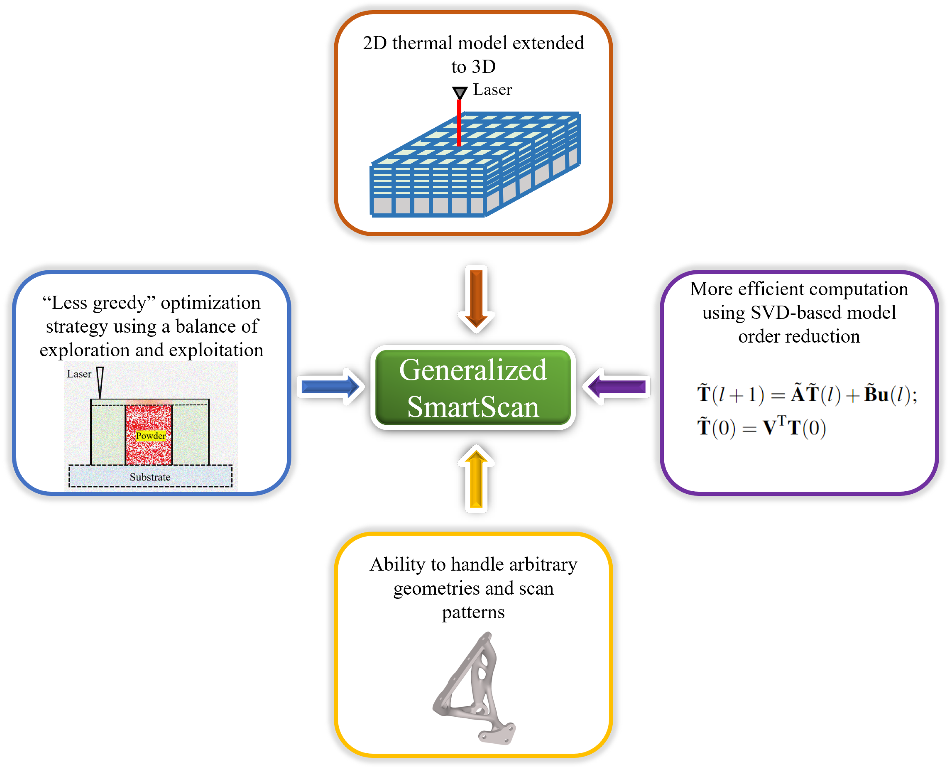
Figure 1. Overview of key features of generalized SmartScan.

Figure 2. Simplified finite difference model of LPBF [31]

Figure 3. (a) Complete and (b) simplified versions of the thermal model adopted for SmartScan in this paper.

Figure 4. The flowchart of the generalized SmartScan.

Figure 5. (a) Cross-sectional view; and (b) top view of the active layer of an example part with an overhang used to demonstrate the greediness problem of the original SmartScan.

Figure 6. (a) Perspective view of a 3D model used in Case Study 1 to show the benefits of probabilistic exploration and SVD-based MOR to generalized SmartScan. (b) Top view of the layer of interest showing the scan pattern.

Figure 7. Simulated thermal uniformity metric (R) and computation time of the layer of interest in Figure 6 for SmartScan with and without probabilistic exploration and/or SVD-based MOR.

Figure 8. Simulated temperature distribution of the layer of interest at four instances (25, 50, 75 and 100% completion) during the scanning process with and without probabilistic exploration.

Figure 9. Printed parts using SmartScan without and with exploration used to validate the benefits of adding exploration on part accuracy.

Figure 10. The scan results of the front surface of the parts printed using SmartScan without and with exploration showing significant improvements in shape accuracy achieved by adding exploration. This benefit is achieved due to reduced local heat accumulation when exploration is added

Figure 11. Cantilever beam geometry used for simulations and experiments in Case Study 2.

Figure 12. Simulated thermal uniformity metric (R) of Layer A for different scan sequences using a bidirectional vector pattern.

Figure 13. Simulated temperature distribution of Layer A at four instances (25, 50, 75 and 100% completion) during the scanning process using a bidirectional vector pattern.

Figure 14. Simulated thermal uniformity metric (R) of Layer B for different scan sequences using a bidirectional vector pattern.

Figure 15. Simulated temperature distribution of Layer B at four instances (25, 50, 75 and 100% completion) during the scanning process using the bidirectional vector pattern.

Figure 16. Printed parts using (a) Sequential, (b) Alternating, and (c) SmartScan sequences and the analysis of the laser scans of their top surfaces for deformation.

Figure 17. Residual stress measurement in cantilever beams.

Figure 18. Complex bracket geometry used for testing SmartScan plug-in: (a) without supports; (b) with supports added by commercial slicer; (c) sample slice of a layer showing fragments that are filled with a hatch pattern.

Figure 19. Comparison of prints of complex bracket geometry obtained using default scan sequence and the optimal scan sequence generated using the SmartScan plug-in to a commercial slicer. The print using the default scan sequence fails while that using SmartScan is successful.

Figure 20. Comparison of the scan sequences of Layer 600 (near the location of the defect in Figure 19) obtained using the default approach of a commercial slicer and SmartScan

Table 1. Parameters used in simulations and experiments.

Parameter (Units)	Value
Laser power, P (W)	290
Laser spot diameter ( $μ m$ )	77
Absorptance, $η$	0.37
Mark/scan speed (mm/s)	1200
Jump speed (mm/s)	6000
Hatch spacing ( $μ m$ )	100
Layer thickness ( $μ m$ )	50
Conductivity, $k_{t}$ ( $\frac{W}{m \cdot K}$ )	22.5
Diffusivity, $α$ ( $\frac{m^{2}}{s}$ )	$5.632 \times 10^{- 6}$
Melting temperature, $T_{m}$ (K)	1658
Convection coefficient, h ( $\frac{W}{m^{2} \cdot K}$ )	25
Ambient temperature, $T_{a}$ (K)	293

Table 2. Printing time for the evaluated scan sequences.

Vector Pattern	Print Time [min]
Sequential	37
Alternating	37
SmartScan	39

Disclaimer/Publisher’s Note: The statements, opinions and data contained in all publications are solely those of the individual author(s) and contributor(s) and not of MDPI and/or the editor(s). MDPI and/or the editor(s) disclaim responsibility for any injury to people or property resulting from any ideas, methods, instructions or products referred to in the content.

© 2024 by the authors. Licensee MDPI, Basel, Switzerland. This article is an open access article distributed under the terms and conditions of the Creative Commons Attribution (CC BY) license (http://creativecommons.org/licenses/by/4.0/).

Copyright: This open access article is published under a Creative Commons CC BY 4.0 license, which permit the free download, distribution, and reuse, provided that the author and preprint are cited in any reuse.

Alerts

MDPI Initiatives

Important Links

Choose an area of interest and we will send you notifications of new preprints at your preferred frequency.

Disclaimer

Generalized SmartScan: An Intelligent LPBF Scan Sequence Optimization Approach for 3D Part Geometries

Abstract

Keywords:

Subject:

1. Introduction

2. Methodology

2.1. Extension of FDM Modeling to Arbitrary 3D Geometries and Scan Patterns

2.2. Objective Function and Optimization

2.3. Relaxation of the Greediness of the Optimization Algorithm

2.4. SVD-based Model Order Reduction

3. Simulation and Experimental Case Studies

3.1. Simulation and Experimental Setup

3.2. Case Study 1: Block with Circular and Diamond-shaped Channels

3.3. Case Study 2: Cantilever Beam

3.4. Case Study 3: Complex 3D Part

4. Conclusions and Future Work

Author Contributions

Acknowledgments

Conflicts of Interest

Abbreviations

Appendix A

Appendix A.1. Validation of the Effectiveness of the Chosen Values for k *

Appendix A.2. Construction of the System Matrix Included in Equation (uid11)

References

MDPI Initiatives

Important Links

Subscribe