1. Introduction
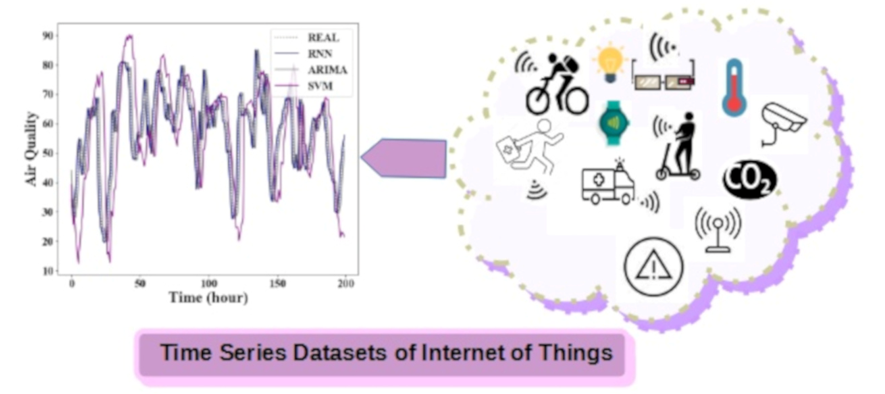
Internet of Things (IoT) is a growing technology development branch in the market, providing solutions in various social an economic aspect through the establishment of development standards on low-operational cost computational systems. IoT can be used in monitoring with sensor devices in different types of scenarios, such as, industry, health, environmental monitoring, smart cities, among others. Indeed, the widespread distribution of these devices implies a large volume of data being continuously created.
Commonly, sensor data are ordered by time, formatted as Time Series. According to [
1], a time series can be defined as a set of observations ordered by time. These observations may demonstrate various behaviors: (i) Trend - Long-term elements related to the time series; (ii) Cycle - Relatively regular waves, around a trend line; (iii) Seasonality - Regular patterns of the time series; (iv) Randomness - Effects that were not incorporated by the time series through the three components cited above. In other words, the residue.
Time series analysis is not only related to the time series behavior identification, but also to the prediction of future values. This feature is important in some contexts, such as reservoirs level monitoring, earthquakes, air quality, among others.
Nowadays, there are different time series prediction models, from the simplest and easy to implement to the most complicated, based on mathematical formalities and statistics involving a great effort in the prediction of future values. As prediction is not a trivial task, it must be combined powerful algorithms, such as those mentioned above, with large data processing capabilities, to reach good results with the least possible response time.
This paper brings as its main contribution a Prediction Model Based in Recurrent Neural Networks (RNN) [
2] for dataset in time series format. Recurrent Neural Networks differ from traditional neural networks (feedforward) because the RNN has the ability to receive signals from both the input layer and the hidden layer in the previous iteration [
2]. In a way, the hidden layer simulates how memory works. Furthermore, RNN works with sequential data in both the input layer and the output layer, fitting perfectly into the context of time series.
In the literature, approaches for predicting time series based on bio-inspired Algorithms, Machine Learning, Big Data, Deep Learning, Neural Networks, and others are found, which have great data processing capacity to achieve good results with the shortest possible response time. As prediction is not a trivial task, this work, in turn, intend to purpose a model easy to implement and capable of dealing with any time-series generated by IoT sensors.
To verify the accuracy of the model, experiments were carried out with five datasets from IoT monitoring applications. It’s them: Data from air quality sensors [
3]; Power consumption data [
4]; Estuarine water quality monitoring data [
5]; Data of Carbon Dioxide emission records [
6]; Dental chairs compressors monitoring [
7]. The proposed solution was compared to the models, Autoregressive Integrated Moving Average (ARIMA) [
8] and Support Vector Machine (SVM) [
9].
The road map of this paper is organized as follows.
Section 2 presents the related work;
Section 3 describes the proposed Prediction Model with Recurrent Neural Networks;
Section 4 presents the results obtained and discussion, and finally, in
Section 5, the conclusions and future work.
2. Current State of the Art
In this section, the background of the work is presented to give a brief context of the model that deal with the problem of time series prediction based on Neural Networks.
2.1. Time Series Prediction
Data Prediction technique aims to estimate future values based on historical data. Based on this principle, the measurements history from a particular sensor node can be used by the sink node to predict future measurements. According to [
10], prediction models can be classified into, statistics-based and machine learning-based.
Regarding statistical models, the Autoregressive Integrated Moving Average (ARIMA) [
11] model stands out. The following stand out among the models based on machine learning:
Support Vector Machine (SVM) [
12] and Recurrent Neural Networks (RNN) [
13].
An autoregressive integrated moving average (ARIMA) model [
11] is a statistical time series forecasting model that aims to find autocorrelations in observations of a given time series in order to make future predictions. According to [
14], the ARIMA model is composed of two models: autoregressive (AR) and moving averages (MA). Autoregressive (AR) and moving average (MA) models deal only with stationary time series [
15]. A time series is stationary if the series mean and the covariance among its observations do not change over time and do not follow trends. Therefore, time series with a tendency or seasonality cannot be considered stationary [
16].
For the prediction of non-stationary time series to be possible, it is necessary to apply differentiation [
17]. Differentiation aims to transform non-stationary time series into stationary time series by calculating the difference between consecutive values of the time series. The differentiation process aims to stabilize the time series average by removing large variations, resulting in the reduction of trend and seasonal behavior. ARIMA is a time series prediction model composed of the combination of autoregressive (AR) and moving average (MA) models, together with the differentiation process.
The
Support Vector Machine (SVM) [
12] is a machine learning technique widely used in different domains, such as text categorization, image analysis and Bioinformatics. SVM has a set of supervised learning methods for data analysis and pattern recognition and can be applied to both classification and regression.
SVR is a derivation of SVM, proposed by [
18], considered a non-parametric technique, as it depends on the use of kernels, which are mathematical functions used to receive input data and transform it into the required form. According to [
19,
20], several
kernels can be used in SVR for time series prediction, such as: linear kernel, radial basis function kernel (Radial Basis Function), least square kernel (Least Square), among others.
Artificial Neural Networks are computational models inspired by biological neural networks. Such models seek to learn how to perform certain tasks through the analysis of examples. Artificial Neural Networks’ main objective is to learn how to solve complex problems in a reasonable amount of time [
21]. Artificial Neural Networks have been massively used in several areas, such as image classification [
22], speech recognition [
23], natural language processing [
24] and time series prediction [
25].
Artificial Neural Networks are composed of an input layer, one or more hidden layers, and an output layer. Each layer contains a certain number of neurons, with each neuron being connected to all neurons in the next layer through synapses. According to [
26], the function of synapses is to assign a weight to transferred data. The neurons in the input layer are responsible for inserting data into the network, while the neurons in the hidden layers receive the weighted sums of their inputs and pass on the new data through a non-linear activation function.
There are neural networks in which connections between neurons form cycles, with the purpose of capturing temporal and contextual information in time series data. These networks are called Recurrent Neural Networks [
27]. Recurrent Neural Networks receive data from the input layer and keep it to be used in the next iteration. The flow of information does not go in one direction, nor does the result depend exclusively on the current input, but also on previous inputs.
[
28] explains that the hidden state of the Recurrent Neural Network receives information from the independent variables, as well as its own processing result from the previous iteration. The activity of neurons in Recurrent Neural Networks is like the behavior of a short-term memory, being very useful in the context of time series prediction, considering that the data from the input and output layers are sequential data.
Data Prediction in Internet of Things can be challenging due to the heterogeneity of the dataset and the volume of monitoring data, which can be massive. To address this challenge, researchers have proposed various data Prediction solutions.
2.2. Related Works
The work presented by [
29], proposes a solution based on single-layer feedforward neural networks with an Online Sequential Learning Algorithm (OSLA). This work presents a mathematical perspective that aims to map the current and previous values through a General Non-Linear System. Comparisons with other models using several datasets are shown and the results confirm that the OSLA obtained better performance than the other models compared.
The paper [
30] proposes a model for predicting multivariate time series using Hierarchical Neural Networks allied to single cycle reservoirs (SCR) and machine learning. The particle swarm optimization algorithm (PSO) is used as training set to optimize SCR parameters. Simulation results show that the proposed model surpasses the other models evaluated. Its hierarchical structure is specially designed to capture the dynamic and complex characteristics of multivariate time series.
In the work [
31], the authors present a method based on Coevolutionary Recurrent Neural Networks for the prediction of chaotic time series with a focus on predictions of many steps ahead. For the training of the neural network, the techniques of Backpropagation Through Time (BPTT) and Cooperative Neuro-Evolution (CNE) were used. For the tests, synthetic and real datasets were used. The results showed that the prediction of many steps ahead is still a great challenge, since the accumulation of errors in the predictions end up with big errors in the results.
In [
32], the authors proposed an adaptive gradient learning method for Recurrent Neural Networks to predict time series with anomalies. The proposed algorithm aims to incrementally learn the time series and provide robust predictions by adapting to changing patterns as well as resisting outliers. Experiments have shown that the proposed approach shows superiority over other methods evaluated.
Although the works mentioned above demonstrate good results, the implementations aim at very specific objectives and are quite complex. This work aims to propose a simple and easy implementation model for the prediction of any type of time series generated by devices from Internet of Things.
3. Time Series Prediction Model with Recurrent Neural Networks
This section describes the proposed solution for time series prediction based on RNN in datasets from IoT sensors.
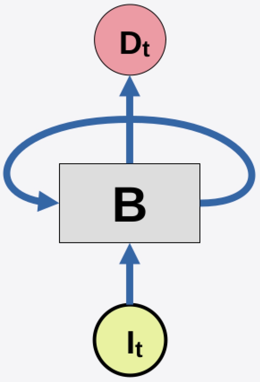
As pointed out in [
33], the RNN receives information from the independent variables, as well as from its own processing result from the previous iteration, as illustrated in
Figure 1.
In this example,
is the input data in the time iteration
t, which is going to be processed by the neuron
B.
is the output from neuron
B in the time iteration
t, that can be used in the next iteration by the same neuron, as a recurrence standard behavior. It is quite similar to the behavior of a short-term memory and it is quite useful in the time series prediction context, given that the data of the input and output layers are sequential [
28].
Neural Networks are commonly used for regression and classification problems. The proposed model uses Recurrent Neural Networks for a regression problem. Which means an equation to estimate the expected value of a variable y, given the values of some other variables i.
When developing the model, we used TensorFlow [
35]. TensorFlow is a project from Google to large scale machine learning models. It’s a flexible dataflow-like programming model and can be applied in different platforms of hardware.
TensorFlow can even be used to express a wide variety of algorithms, including training algorithms for scalable neural networks. The main Application Programming Interface (API) is in the Python programming language and in C ++ [
35]. TensorFlow supports both CPU and GPU processing to reach higher level of parallelization in executions. In this work, the Python programming language was used, together with some libraries used for data manipulation, such as Pandas [
36], NumPy [
37] and MatPlotLib [
38].
3.1. Definition of Cost Function and Metrics
In Machine Learning, there is a cost, also called
loss, which is related to the learning process. [
28] states that this cost is represented by the size of the obtained error according to the parameter values that were used. Effectively, cost is the obtained deviation size to specific parameters set. In this case, it is necessary minimize the cost function so that the learning process can be improved.
The Gradient Descent method is used in optimization for the purpose of minimize the cost function using an iterative scheme. Given that the function in question is convex, the negative direction of the gradient is taken at each iteration, until the overall minimum is reached. Nevertheless, the Gradient Descent method may not be ideal when the data set is very large, because the algorithm would loop through the whole data set to compute the gradient and make just one move towards the optimization process.
Since IoT data is massive, in this work it was used the Stochastic Gradient Descent method [
39]. In this method, mini batches of data are created randomly to be looped through the algorithm. Consequently, it is not necessary to loop through the entire data set to compute the gradient. It is possible to obtain an approximation just looping through some examples of the data set. However, to get closer of the global minimum, it will be necessary a great number of iterations. Either way, the time of each iteration should be remarkably short, and the learning should be faster [
39]. It is common to find this method being used for training of Neural Networks and linear regression problems and this motivated the use of this method in our work.
When evaluating the accuracy of the prediction model, some metrics need to be defined. The most used metrics in machine learning are the Mean Absolute Error (MAE) and the Coefficient of Determination ().
The MAE measures the average distance from the predictions related to the observed values, focusing the estimation on the conditional median. The coefficient of determination measures the adjustment of a generalized linear statistical model, such as linear regression, in relation to the observed values. The value of
vary between 0 and 1, indicating in percentage, how much the model can explain the observed values [
40].
4. Performance Evaluation
In this section, we present results of experiments conducted on a computer with the following characteristics: AMD Phenom (tm) II X4 B93 Processor with 4 cores and 4Gb of RAM running Ubuntu Linux 16.04.
The results obtained with the proposed approach in
Section 3 are compared with the results obtained by the Autoregressive Integrated Moving Average (ARIMA) [
8] and the Support Vector Machine (SVM) [
9] algorithms. All models were implemented with the Python programming language.
In experiments, five datasets from Internet of Things were used:
Data from air quality sensors - University of California, Irvine [
3].
Power consumption data from Low Carbon London Project - UKPN [
4].
Burnett river estuarine water quality monitoring data - Queensland Government (Australia) [
5].
Globally averaged Carbon Dioxide emission records - Earth System Research Laboratory (U.S. Federal Government) [
6].
Dental chairs compressors monitoring [
7]. Often, a portion of the air compressors suffer condensation, and the compressors get full of water, leading to the need to purge the water.
Table 1 presents the details of each dataset in terms of sampling, period and number of samples.
In the tests carried out, the aim is to identify whether the model can predict one step ahead according to the latest data observed in each data set.
4.1. Training and Test sets
When a RNN receives sequential data in the input layer, each data sample needs to be a sequence whose format is composed by time periods and variables. As a result, once various data samples are stacked, the mini batches will show a three-dimensional aspect: number of samples, time and variables. In this way, it will be possible to submit the data to the training and test sets. Therefore, each mini batch must contain the discrepancy of one or more rows so that the data maintains the sequential pattern.
To obtain an accurate approximation of the real scenario, it is necessary to split the last data from the time series for the test set. Thus, we defined that the first 70% of each dataset would be used as the training set and the last 30% would be used for the set test.
Since the Stochastic Gradient Descent method is used in the proposed model, it is necessary to shuffle the mini batches for the training set so that the cost function can be optimized. It is possible to choose randomly the number of iterations for the training set. It was observed that the iterations number for the mean absolute error varies according to each dataset.
The parameter related to the number of iterations for the training set was implemented in an online and deterministic way, based on [
41]. The algorithm measures the mean absolute error and concludes the training set if the error doesn’t decrease after a certain number of iterations. The value of this parameter was specified as 20.
Other parameters from the RNN were adjusted: number of neurons, learning rate and mini-batches size. The adjustment was performed in the offline way, that is, before the algorithm execution. These values were chosen empirically, based on algorithm behavior. They are: number of neurons: 64; Learning Rate: 0.001 and finally, mini batches size: 64.
The ARIMA model parameters were defined based on [
14]:
and
q, with
p being the number of delay observations included in the model,
d the degree of differentiation and
q the size of the moving average window. The algorithm implemented in ARIMA follows the steps: (i) Call the
function and pass the parameters
and
q; (ii) Define the training data using the
function; (iii) Make predictions by calling the
function, which performs the one-step-ahead forecast.
The SVM model [
12] is made up of a set of supervised learning methods used for classification and regression. To deal with the regression problem the Support Vector Regression (SVR) [
18] method was used. Therefore, it is necessary to define the SVR
kernel function. In this implementation, the RBF [
20] kernel was used.
4.2. Results and Analysis
In this section, we present results of experiments based on real datasets from Internet of Things monitoring applications. Specifically, only the last 10,000 detections from the air compressor monitoring dataset were used to predict future values, because it is an extensive dataset (almost four million detections). The remaining datasets were used in their entirety. In the results, the confidence interval is 95%.
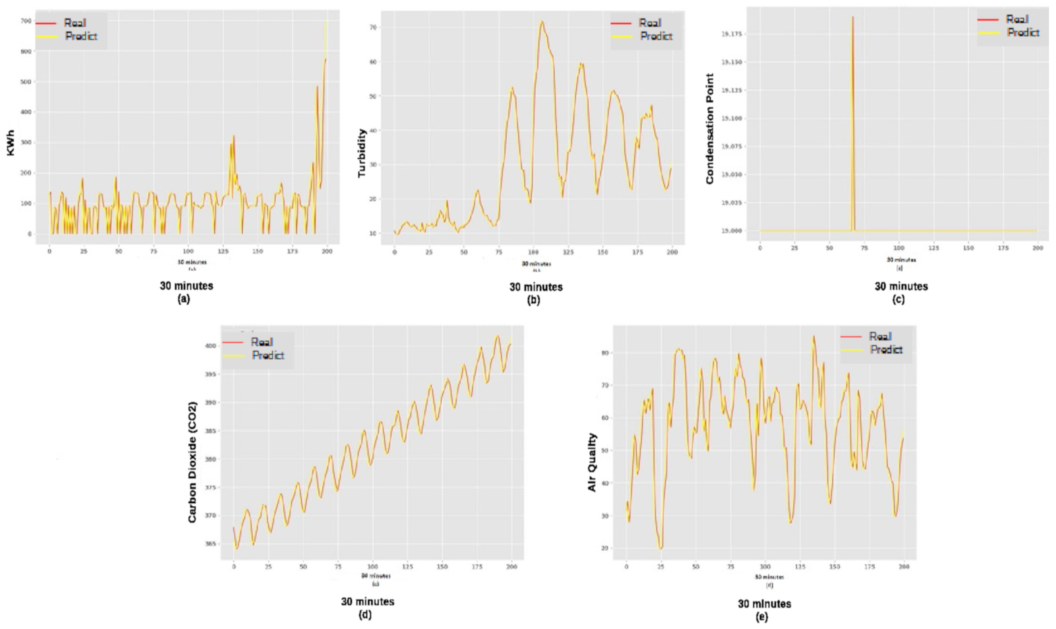
The
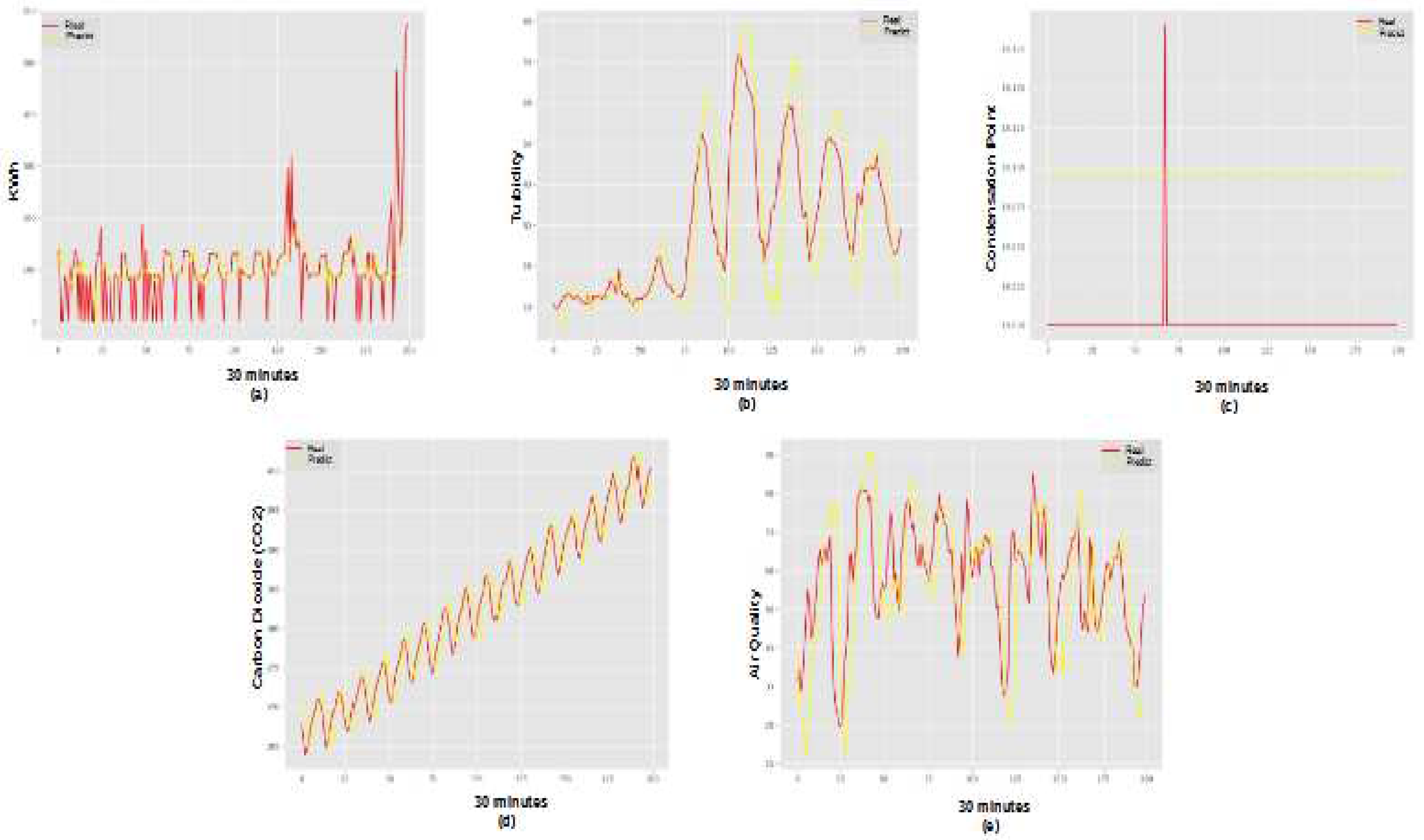
Figure 2 presents the results of predictions, Real and Predicted, obtained with the Recurrent Neural Networks (of the following datasets: SmartMeter (a), Water Quality (b), Dental Compressors (c), CO2 Emission (d) and Air Quality (e).
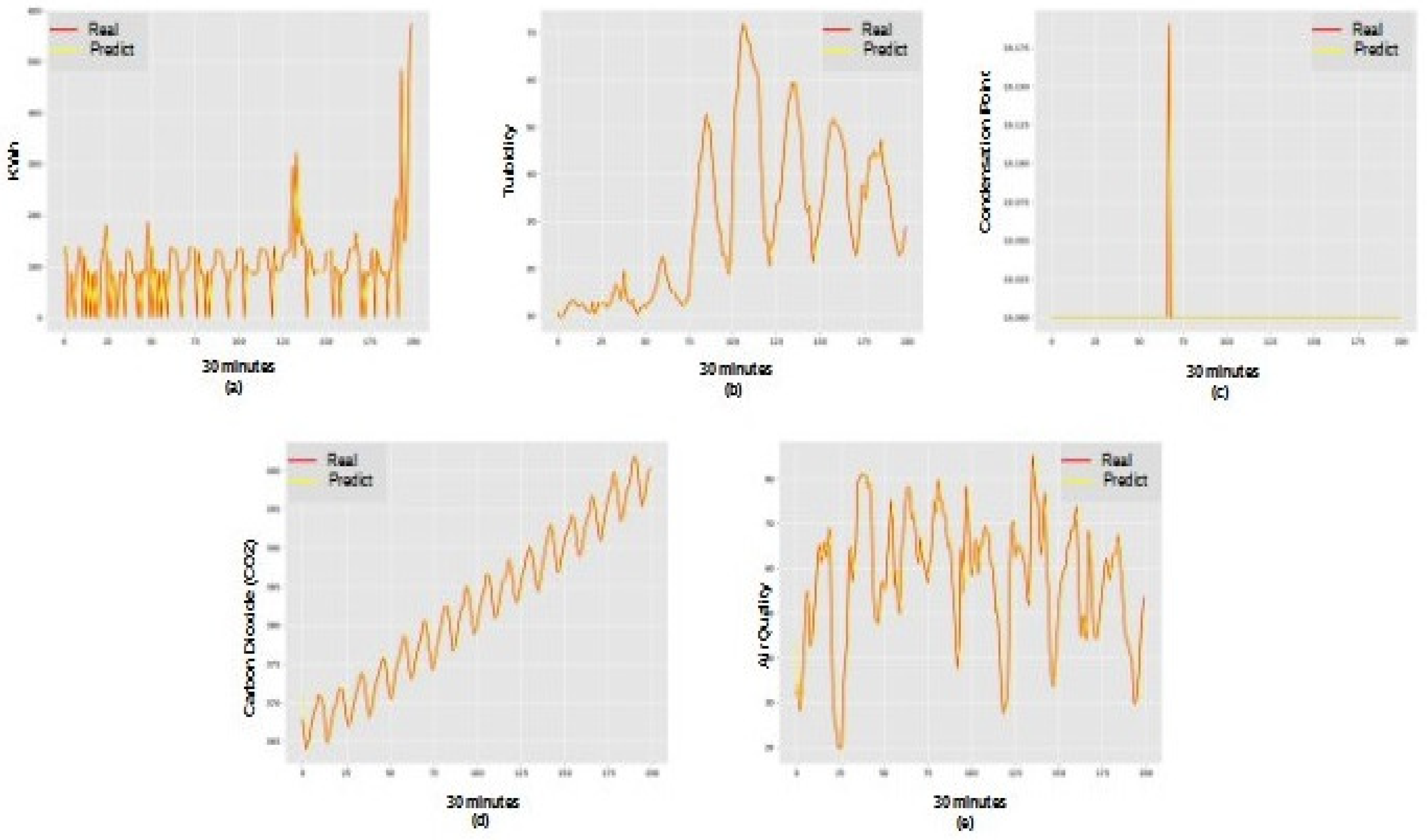
Based on the results, it was found that the prediction model with Recurrent Neural Networks finds it difficult to deal with values positioned at the ends of the series. Therefore, prediction in series with predominantly seasonal behavior may not achieve the best possible performance. The ARIMA model (
Figure 3), in turn, demonstrates more assertiveness in predicting values positioned at the extremities, but ends up accumulating errors throughout the series, demonstrating a lower final performance than the Neural Network in this context.
However, compared with ARIMA (see
Figure 3) and SVM (see
Figure 4) models, the Recurrent Neural Network obtains better results. For instance, from the results with Turbidity (Burnett River) time series, it was found that, the model based on ARIMA obtained a lower value of Mean Absolute Error (MAE), but the model based on Recurrent Neural Network reached the highest level of Coefficient of Determination (
).
Regarding the execution time, results in
Figure 5 show that the ARIMA model was faster than Recurrent Neural Network model. This behavior in the Recurrent Neural Network model is explained by the fact that the execution time comprises the training and test phases. Furthermore, the number of iterations in the training set depends on minimizing the Mean Absolute Error (EAM), which can lead to a very high number of iterations.
Based on the search results in
Figure 5a, it appears that SVM models generally outperform ARIMA models in terms of processing time. It has been identified that the time taken by the SVM algorithm to completion is directly proportional to the size of the training set.
The box plots presented in
Figure 5b and
Figure 5c demonstrate the variation in observed data of Mean Absolute Error (EAM), Coefficient of Determination (
) through quartiles. The time series prediction model with Recurrent Neural Networks achieved the lowest mean of Mean Absolute Error and the highest mean of Coefficient of Determination.
In
Figure 5c, in certain cases, the values obtained were negative, demonstrating the low quality of the prediction. According to [
42], in cases where negative values of
arise, the average of the actual data provides a better fit to the results than the values predicted by the prediction model.
Table 2 shows the values of Mean Absolute Error (MAE), Coefficient of Determination (
) and Execution Time (ET) obtained in the prediction from evaluated datasets. The model based on Recurrent Neural Network was executed 10 times for each dataset. The values presented in RNN column represent the average of the executions.
Statistical tests were performed to investigate the statistical difference between the results obtained from the EAM in each model presented in
Table 2. The results do not follow a normal distribution, and it was identified, with a confidence interval calculated at 95%, that there is a statistical difference in the results obtained by the prediction models. The SVM model obtained the best result, followed by the Recurrent Neural Network and the ARIMA model, respectively.
In summary, the results presented regarding Prediction in the evaluated IoT datasets, EAM, and execution time with the models, RNN, ARIMA and SVM indicate that the Recurrent Neural Networks may have some difficulties in dealing with outliers. It is concluded that, the predictions of predominantly seasonal behavior series may not perform well with Recurrent Neural Network.
On the other hand, the model ARIMA presents better accuracy in dealing with outliers, but ends up accumulating errors throughout the time series, presenting an inferior performance regarding the EAM when compared with the RNN.
5. Conclusion
This paper presented a time series prediction model based on Recurrent Neural Networks implemented with the Stochastic Gradient Descent method to minimize cost. RNN was compared to the models, Auto-Regressive Integrated Moving Average (ARIMA) and Support Vector Machine (SVM). In the experiments, real datasets from IoT applications were used. We analyzed the prediction for many steps ahead with the optimization of the Mean Absolute Error and Coefficient of Determination.
The model based on the Recurrent Neural Network obtained better performance when compared to the SVM model, which attained higher Mean Absolute Error (MAE) and lower Coefficient of Determination ().
As future work, it is suggested to improve the model so that it can use the multi-variety of the time series to obtain more assertive predictions in seasonal series. Also, to carry out new comparative tests with other datasets that demonstrate different behaviors (cycle, tendency, randomness).
References
- Morettin, P.A.; de Castro Toloi, C.M. Modelos para previsão de séries temporais; Vol. 1, Instituto de Matemática Pura e Aplicada: Rio de Janeiro, 1981.
- Sundermeyer, M.; Ney, H.; Schlüter, R. From Feedforward to Recurrent LSTM Neural Networks for Language Modeling. IEEE/ACM Transactions on Audio, Speech, and Language Processing 2015, 23, 517–529.
- Vito, S.D.; Massera, E.; Piga, M.; Martinotto, L.; Francia, G.D. On field calibration of an electronic nose for benzene estimation in an urban pollution monitoring scenario. Sensors and Actuators B: Chemical 2008, 129, 750–757.
- Networks, U.P. SmartMeter Energy Consumption Data in London Households. https://data.london.gov.uk/dataset/smartmeter-energy-use-data-in-london-households, 2015. [Accessed: 08/03/2018].
- Queensland Government. Ambient estuarine water quality monitoring data (includes near real-time sites) - 2012 to present day. https://data.qld.gov.au/dataset/ambient-estuarine-water-quality-monitoring-data-near-real-time-sites-2012-to-present-day, 2015. [Accessed: 08/03/2018].
- Dlugokencky, E.; Tans, P. Trends in Atmospheric Carbon Dioxide. https://www.esrl.noaa.gov/gmd/ccgg/trends/gl_data.html, 2017. [Accessed: 08/03/2018].
- Castañeda, W.A.C. Metodologia de gestão ubíqua para tecnologia médico-hospitalar utilizando tecnologias pervasivas. PhD thesis, Federal University of Santa Catarina, Florianópolis, Brazil, 2016.
- Wu, J.; Wei, S. Time series analysis; Hunan Science and Technology Press, ChangSha, 1989.
- Smola, A.J.; Schölkopf, B. A tutorial on support vector regression. Statistics and computing 2004, 14, 199–222.
- Boukary, N.A. A COMPARISON OF TIME SERIES FORECASTING LEARNING ALGORITHMS ON THE TASK OF PREDICTING EVENT TIMING. PhD thesis, Royal Military College of Canada, 2016.
- Box, G.E.; Jenkins, G.M.; Reinsel, G.C.; Ljung, G.M. Time series analysis: forecasting and control; John Wiley & Sons: San Francisco, CA, 2015.
- Sapankevych, N.I.; Sankar, R. Time Series Prediction Using Support Vector Machines: A Survey. IEEE Computational Intelligence Magazine 2009, 4, 24–38. [CrossRef]
- He, X.; Xu, S. Artificial neural networks. Process Neural Networks: Theory and Applications 2010, pp. 20–42.
- Marcellino, M.; Stock, J.H.; Watson, M.W. A comparison of direct and iterated multistep AR methods for forecasting macroeconomic time series. Journal of Econometrics 2006, 135, 499 – 526.
- Deb, C.; Zhang, F.; Yang, J.; Lee, S.E.; Shah, K.W. A review on time series forecasting techniques for building energy consumption. Renewable and Sustainable Energy Reviews 2017, 74, 902 – 924.
- Farhath, Z.A.; Arputhamary, B.; Arockiam, D.L. A Survey on ARIMA Forecasting Using Time Series Model, 2016.
- Hyndman, R.J.; Athanasopoulos, G. Forecasting: principles and practice; OTexts, 2018.
- Drucker, H.; Burges, C.J.; Kaufman, L.; Smola, A.J.; Vapnik, V. Support vector regression machines. In Proceedings of the Advances in neural information processing systems, 1997, pp. 155–161.
- Rüping, S. SVM kernels for time series analysis. Technical report, Technical Report, SFB 475: Komplexitätsreduktion in Multivariaten Datenstrukturen, Universität Dortmund, 2001.
- Rubio, G.; Pomares, H.; Herrera, L.J.; Rojas, I. Kernel Methods Applied to Time Series Forecasting. In Computational and Ambient Intelligence; Springer Berlin Heidelberg, 2007; pp. 782–789.
- van Gerven, M.; Bohte, S. Artificial neural networks as models of neural information processing; Frontiers Media SA, 2018.
- Fadaeddini, A.; Eshghi, M.; Majidi, B. A deep residual neural network for low altitude remote sensing image classification. In Proceedings of the 2018 6th Iranian Joint Congress on Fuzzy and Intelligent Systems (CFIS), Kerman, Iran, Feb 2018.
- Lokesh, S.; Malarvizhi Kumar, P.; Ramya Devi, M.; Parthasarathy, P.; Gokulnath, C. An Automatic Tamil Speech Recognition system by using Bidirectional Recurrent Neural Network with Self-Organizing Map. Neural Computing and Applications 2018. [CrossRef]
- Goldberg, Y. Neural Network Methods for Natural Language Processing. Synthesis Lectures on Human Language Technologies 2017, 10, 1–309.
- Lang, K.; Zhang, M.; Yuan, Y.; Yue, X. Short-term load forecasting based on multivariate time series prediction and weighted neural network with random weights and kernels. Cluster Computing 2018.
- Dertat, A. Applied Deep Learning - Part 1: Artificial Neural Networks. https://towardsdatascience.com/applied-deep-learning-part-1-artificial-neural-networks-d7834f67a4f6, 2017. [Online; acessado em: 14/09/2018].
- Liu, Z.; Sullivan, C.J. Prediction of weather induced background radiation fluctuation with recurrent neural networks. Radiation Physics and Chemistry 2018.
- Goodfellow, I.; Bengio, Y.; Courville, A. Deep Learning; MIT Press, 2016. http://www.deeplearningbook.org.
- George, K.; Mutalik, P. A Multiple Model Approach to Time-Series Prediction Using an Online Sequential Learning Algorithm. IEEE Transactions on Systems, Man, and Cybernetics: Systems 2017, PP, 1–15. [CrossRef]
- Xu, M.; Han, M.; Wang, X. Hierarchical neural networks for multivariate time series prediction. In Proceedings of the 2016 35th Chinese Control Conference (CCC), July 2016, pp. 6971–6976. [CrossRef]
- Hussein, S.; Chandra, R.; Sharma, A. Multi-step-ahead chaotic time series prediction using coevolutionary recurrent neural networks. In Proceedings of the 2016 IEEE Congress on Evolutionary Computation (CEC), July 2016, pp. 3084–3091. [CrossRef]
- Guo, T.; Xu, Z.; Yao, X.; Chen, H.; Aberer, K.; Funaya, K. Robust Online Time Series Prediction with Recurrent Neural Networks. In Proceedings of the 2016 IEEE International Conference on Data Science and Advanced Analytics (DSAA), Oct 2016, pp. 816–825. [CrossRef]
- Barreto, J.M. Introduçaoas redes neurais artificiais. V Escola Regional de Informática. Sociedade Brasileira de Computaçao, Regional Sul, Santa Maria, Florianópolis, Maringá 2002, pp. 5–10.
- Olah, C. Understanding LSTM Networks. http://colah.github.io/posts/2015-08-Understanding-LSTMs/, 2014. [Accessed: 06/12/2017].
- Abadi, M.; Agarwal, A.; Barham, P.; Brevdo, E.; Chen, Z.; Citro, C.; Corrado, G.S.; Davis, A.; Dean, J.; Devin, M.; et al. Tensorflow: Large-scale machine learning on heterogeneous distributed systems. arXiv preprint arXiv:1603.04467 2016.
- McKinney, W.; et al. Data structures for statistical computing in python. In Proceedings of the Proceedings of the 9th Python in Science Conference. Austin, TX, 2010, Vol. 445, pp. 51–56.
- Harris, C.R.; Millman, K.J.; van der Walt, S.J.; Gommers, R.; Virtanen, P.; Cournapeau, D.; Wieser, E.; Taylor, J.; Berg, S.; Smith, N.J.; et al. Array programming with NumPy. Nature 2020, 585, 357–362. [CrossRef]
- Hunter, J.D. Matplotlib: A 2D graphics environment. Computing In Science & Engineering 2007, 9, 90–95.
- Bottou, L. Large-scale machine learning with stochastic gradient descent. In Proceedings of COMPSTAT’2010; Springer, 2010; pp. 177–186.
- Nagelkerke, N.J. A note on a general definition of the coefficient of determination. Biometrika 1991, 78, 691–692.
- André, L.; Parpinelli, R.S. Tutorial Sobre o Uso de Técnicas para Controle de Parâmetros em Algoritmos de Inteligência de Enxame e Computação Evolutiva. Revista de Informática Teórica e Aplicada 2014, 21, 90–135.
- Imdadullah, M. Coefficient of Determination: A model Selection Criteria. http://itfeature.com/correlation-and-regression-analysis/coefficient-of-determination, 2012. [Online; acessado em 13/07/2018].
|
Disclaimer/Publisher’s Note: The statements, opinions and data contained in all publications are solely those of the individual author(s) and contributor(s) and not of MDPI and/or the editor(s). MDPI and/or the editor(s) disclaim responsibility for any injury to people or property resulting from any ideas, methods, instructions or products referred to in the content. |
© 2023 by the authors. Licensee MDPI, Basel, Switzerland. This article is an open access article distributed under the terms and conditions of the Creative Commons Attribution (CC BY) license (http://creativecommons.org/licenses/by/4.0/).
