Submitted:
06 November 2023
Posted:
06 November 2023
You are already at the latest version
Abstract
In this paper, intrusion detection systems are thoroughly investigated utilizing the CSE-CIC-IDS-2018 dataset. The research is divided into three key phases: first, applying Data Cleaning, Exploratory Data Analysis, and Data Normalization techniques (min-max and z-score) for preparing data across distinct classifiers. Second, feature importance is reduced using a combination of Principal Component Analysis (PCA) and Random Forest (RF), with the goal of improving processing speed and decreasing model complexity. This stage comprises a comparison with the entire dataset. Finally, machine learning algorithms (XGBoost, CART, DT, KNN, MLP, RF, LR, and Bayes) are applied to specific features and preprocessing approaches. Surprisingly, the XGBoost, DT, and RF models outperform in both ROC values and CPU runtime. Following evaluation, which includes PCA and RF feature selection, an optimal set is produced.
Keywords:
intrusion detection system
; machine learning techniques
; Exploratory Data Analysis
; Performance Evaluation
; feature selection
; CSE-CIC-IDS-2018 dataset
; Three phase models
1. Introduction
In today’s world, the Internet has become an invaluable tool, effortlessly integrated into human life. People all over the world utilize it as a communication and information exchange medium. Information and communication technology (ICT) is essential in both business and daily life. However, in the age of big data, cyber-attacks on ICT systems have become increasingly sophisticated and broad, making network risks a key issue in modern life. Malicious attacks are continually developing, emphasizing the critical need for improved network security solutions. Given the world’s growing reliance on digital technologies such as computers and the Internet, building safe and reliable programs, frameworks, and networks that can withstand these attacks is a critical task [1,2].
Intrusion detection systems (IDS) are critical for protecting computer networks. They effectively recognize and respond to security threats. Intrusion it used to detect irregularities in network traffic to improve security. Detection accuracy, detection times, false alarm alerts, and the identification of unknown assaults are currently issues for IDS technology [3] They are classified into three types: signature-based systems, anomaly-based systems, and hybrid systems. Anomaly-based systems can detect unknown hostile actions by recognizing deviations from a model based on typical behavior, whereas signature-based systems can identify known assaults by employing established signatures. Signature-based systems, on the other hand, have a high rate of false alarms [4]. Existing anomaly intrusion detection systems have accuracy problems. Certain datasets lack network traffic diversity and volume, others lack diverse or recent attack patterns, and still others lack crucial feature set metadata. The hybrid IDS, which includes both anomaly-based and misuse-based IDSs, proved to be a more robust and effective solution. Network Intrusion Detection Systems (NIDS) are critical in resolving security issues. NIDS monitors network traffic for unusual activity, then analyzes the data to discover security breaches such as invasions, misuse, and anomalies. NIDS must deal with difficulties like large data dimensionality and high traffic volumes [5]. While many research projects have used machine learning techniques approaches are useful in NIDS, they have limits when confronted with large amounts of network data. Feature selection (FS) has become widely used in selecting relevant features for building strong models. It has significantly influenced the efficiency and performance of IDS models [6]. As a result, three critical aspects of NIDS development are preprocessing, feature reduction, and classifier methods. Nonetheless, network intrusion detection systems encounter issues such as managing massive amounts of data, high false alarm rates, and skewed data.
Machine learning techniques (ML) have been widely. It used in the field of information security in recent years. ML have found widespread application in network security during the last two decades [7]. ML approaches are becoming more popular as a method of spotting anomalies [8]. ML includes automating the process of learning from examples. It is used to build models that distinguish between regular and aberrant classes [9].
The goal of this study was to find the most effective classifier by Methods for preprocessing and feature selection are translated into machine learning approaches that are extensively used by we in intrusion detection systems. Popular classification algorithms such as eXtreme Gradient Boosting (XGBoost), Classification and Regression Trees (CART), Decision Tree (DT), k-Nearest Neighbors (KNN), Multilayer Perceptron (MLP), Random Forest (RF), Logistic Regression (LR), and Naïve Bayes (Bayes) are included. The evaluation of performance encompasses several dimensions as nine important criteria: In average accuracy k-fold cross-validation, accuracy, precision, recall, F1 score, PCC/BA, MCC, ROC, and average were calculated. Classification CPU Time and Model Size.
The following are the main contributions of this study:
- Investigation of large amounts of data linked with harmful network activity.
- Identification of feature dimensions influencing classification performance in a labeled dataset with both benign and malicious traffic, resulting in improved detection accuracy.
- Use of the CSE-CIC-IDS-2018 dataset for NIDS and testing of seven different machine learning classifiers and scripts for identifying various sorts of assaults.
- In general, researchers frequently work with incomplete data. In contrast, this study uses all accessible DDoS data in the experiment, correlating with reality by adopting the concept of data imbalance.
- Presenting various performance assessments has many elements. Furthermore, the evaluation considers CPU processing time, which is an important component in intrusion detection, as well as the size of the experimentally obtained model, which has the possibility for future extension.
The rest of the paper is structured as follows: Section 2 describes the research sequence, as well as the research concept and process. The methodology and proposed framework are described in Section 3. The experimental setup is described and defined in Section 4. The experiments and related discussions are presented in Section 5. Finally, Section 6 concludes the essay by discussing the model’s strengths and flaws and suggesting future study directions.
2. Related work
There are very few datasets for network intrusion detection compared to datasets for malicious code. KDD CUP 99 (KDD) is the most widely used dataset for the evaluation of IDS. Numerous studies on ML-based IDS have been using KDD or the upgraded versions of KDD. In this work, we develop an IDS model using CSE-CIC-IDS-2018, a dataset containing the most up-to-date common network attacks [10]. The Canadian Institute for Cybersecurity’s CSE-CIC-IDS-2018 dataset incorporates the concept of profiles. The most recent edition of this dataset provides versatility, allowing both agents and individuals to generate network events. These profiles can be applied to a variety of network protocols and topologies. Furthermore, the dataset has been updated by adding the standards used in the development of CIC-IDS-2017. In addition to meeting the necessary requirements, it provides the following benefits: minimum duplicate data, nearly no unclear information, and the dataset is already in CSV format, making it ready for use without further processing [11].
As data dimensionality grows, feature selection has become a critical preprocessing step in the development of intrusion detection systems. Feature selection entails removing irrelevant and superfluous features and picking the optimal subset that best characterizes patterns in various classes. There are various advantages to feature selection. It reduces feature dimensionality, which leads to better algorithm performance. By removing redundant, irrelevant, or noisy data, it improves data efficiency and thus learning technique performance. It also improves the correctness of the output model and aids in understanding the underlying operations that generated the data [12,13].
Following a study of relevant documents and research articles, it was discovered that several studies used Machine Learning techniques in conjunction with the CEC-CIC-IDS- 2018 dataset to detect intrusions. The following is an overview of these findings:
- S. Ullah et al. [14].proposed comparing some of the most efficient machine learning algorithms RF, Bayes, LR, KNN, DT and feature selection by RF (30 features). Use CSE-CIC-IDS-2018 dataset. The research results showed that the decision tree had the most results.
- Khan [15] developed a HCRNNIDS: Hybrid Convolutional Recurrent Neural Network-Based NIDS and feature selection by RF (30 features). Compare with machine learning algorithms DT, LR and XGBoost. Use CSE-CIC-IDS-2018 dataset. The research results showed that the HCRNNIDS had the most results.
- Kim et al. [10] discuss the creation and testing of IDS models using various machine learning algorithms such as artificial neural networks (ANN), support vector machines (SVM), and deep learning approaches such as convolutional neural networks (CNN) and recurrent neural networks (RNN). When applied to datasets such as CSE-CIC-IDS-2018, the experimental results suggest that machine learning models, notably CNN, outperform traditional techniques.
- R. Qusyairi et al. [3] suggest an ensemble learning technique that incorporates various detection algorithms. LR, DT, and gradient boosting were chosen for the ensemble model after comparisons with single classifiers. The study identified 23 significant traits out of 80 using the CSE-CIC-IDS-2018 dataset.
- S. Chimphlee et.al. [4] focuses on Intrusion Detection Systems (IDS) and presents an efficient classification scheme using the CSE-CIC-IDS-2018 dataset. The study examined the best-performing model for classifying invaders by using data preprocessing approaches such as under-sampling and feature selection, as well as seven classifier machine learning algorithms. Notably, the study investigated the use of random forest (RF) for feature selection as well as machine learning approaches such as MLP and XGBoost. According to the experimental results, MLP provided the most successful and best-performing outcomes based on evaluation parameters.
As a result, previous researchers investigated a variety of techniques based on standard machine learning for intrusion detection.
3. Methods
We learn about the problem and its solutions by studying information and relevant research publications. This knowledge has been translated by the we into a framework, which is illustrated in Figure 1, and is divided into three distinct phases. The study makes use of standardized data and is primarily concerned with intrusion detection systems. It specifically makes use of the CSE-CIC-IDS-2018 dataset [16]. Data Cleaning, Exploratory Data Analysis, and Data Normalization employing two techniques: min-max normalization and z-score normalization are all part of the Data Preprocessing process in Phase 1. This is done to evaluate the effectiveness of these strategies when applied to different classifier models. Following that, the research moves on to Phase 2, which involves assessing the significance of each feature in the experimental dataset. The goal here is to reduce data complexity, which improves both processing speed and model size. This is accomplished by combining two techniques: Principal Component Analysis (PCA) [17] and Random Forest (RF) [18]. The investigation includes using the complete dataset without feature reduction, allowing for a comparison of their efficiency when applied to multiple classifier models. In the final phase, the dataset, which has undergone Data Preprocessing and Feature Selection based on predetermined criteria, is used with machine learning algorithms chosen by the we common classification techniques such as XGBoost [19], CART [20], DT [21], KNN [22], MLP [23], RF [24], LR [25], and Bayes [26] are used to assess performance across multiple dimensions, as mentioned in the following section.
4. Experimental Setup
This study used a 64-bit Windows operating system (Windows 11) with the following specifications: an 11th Gen Intel(R) Core(TM) i7-11800H at 2.30GHz, 32 GB of 2933 MHz DDR4 Memory. The Python 3.11 environment was utilized, and the recommended model was implemented and evaluated using the Numpy, pandas, and sklearn data preparation tools. Pandas and Numpy libraries were used for data handling, preprocessing, and analysis, while Scikit Learn was used for model training, evaluation, and evaluation metrics. The Seaborn package and Matplotlib were used to visualize the data. The subsections that follow go into greater detail.
4.1. CSE-CIC-IDS-2018 Data Set
The data set given for the CSE-CIC-IDS-2018 [16] was developed through a collaborative project between the Communications Security Establishment (CSE) and the Canadian Institute for Cybersecurity (CIC). It was created with the goal of evaluating intrusion detection research, and it has now become a benchmark data set for the evaluation of IDSs. The data was obtained a ten-day period, eighty columns, and There are fifteen sorts of attacks: FTP-BruteForce, SSH-Bruteforce, DoS attacks-GoldenEye, DoS attacks-Slowloris, DoS attacks-Hulk, DoS attacks-SlowHTTPTest, DDoS attacks-LOIC-HTTP, DDOS attack-HOIC, DDOS attack-LOIC-UDP, Brute Force-Web, Brute Force-XSS, SQL Injection, Infilteration, Label and Bot. The study focuses on DDoS intrusions [14], because a difficult type of assault to counter. We found and use that the data contained DDoS intrusion types for 2 days, namely 02-20-2018.csv and 02-21-2018.csv.
4.2. Data Preprocessing
4.2.1. Data Cleaning
We chose two unique days’ datasets, 02-20-2018.csv (with 84 features) and 02-21-2018.csv (with 80 features). To normalize the dataset, we reduced it to 80 features after removing the first four: Flow ID, Src IP, Src Port, and Dst IP. These excluded attributes from the two days were combined. Machine learning models were created using the remaining 84 features and compared to models created using the reduced 80 features. The primary focus was on DDoS attacks. The labels were divided into four categories, yielding a dataset of 8,997,323 rows and 80 columns. Label 0 denotes benign, Label 1 denotes DDoS attacks-LOIC-HTTP, Label 2 denotes DDOS attacks-HOIC, and Label 3 denotes DDOS attacks-LOIC-UDP.
4.2.2. Exploratory Data Analysis
The analysis included determining the minimum, maximum, standard deviation, and mean values of the data for all 80 attributes, including the labels. Bwd PSH Flags, Fwd URG Flags, Bwd URG Flags, CWE Flag Count, Fwd Byts/b Avg, Fwd Pkts/b Avg, Fwd Blk Rate Avg, Bwd Byts/b Avg, Bwd Pkts/b Avg, and Bwd Blk Rate Avg were all removed. Additionally, features of the Timestamp type defined as Object were eliminated to improve classification appropriateness. To prepare the dataset for classification, the feature with the Timestamp type classified as Object was eliminated. This change was made to improve the dataset’s usability for classification applications. The initial dataset contained 8,997,323 rows and 69 characteristics. To assure data quality, several procedures were done, including the removal of NaN values (36,767 rows), the elimination of +inf and -inf values (22,686 rows), and the deletion of duplicate rows (2,302,927 rows). The dataset was refined to 6,634,943 rows after cleaning operations that included deleting NaN, +-inf values, and duplicates, making it ready for future study and use.
The Table 1 displays data statistics before and after cleaning. Initially, there were 8,997,323 rows grouped into different labels, with “Benign” accounting for 85.95% of the records, “DDoS attacks-LOIC-HTTP” accounting for 6.40%, “DDOS attack-HOIC” accounting for 7.62%, and “DDOS attack-LOIC-UDP” accounting for 0.02%. The dataset was cleaned and reduced to 6,634,943 rows. “Benign” entries made up 88.31% of the cleaned data, indicating a reduction from the original dataset. “DDoS attacks-LOIC-HTTP” and “DDOS attack-HOIC” percentages increased somewhat, while “DDOS attack-LOIC-UDP” remained at 0.03%. These modifications represent the effect of data cleansing on the distribution of the various attack categories.
4.2.3. Data Normalization
Normalization is used in data preparation step of Machine Learning to standardize numerical column values and ensure they are on a consistent scale [27]. Normalization, a transformation method, improves a model’s performance and accuracy greatly, especially when the distribution of information is uncertain. Without a consistent pattern, effective Normalization relies on large datasets to smooth data by removing outliers. This technique, which is critical in data preprocessing for Network Intrusion Detection Systems (NIDS), standardizes data to a given scale, often ranging from 0 to 1. This ensures that all features have consistent scales and ranges, thereby improving the performance and accuracy of NIDS. Several normalization approaches are employed in data pre-processing. Some of the most common are [28].
- Min Max Normalization: This approach reduces the values of a feature to a range between 0 and 1. It accomplishes this by subtracting the minimum value of the feature from each data point and then dividing the result by the range of the feature. This technique’s equivalent mathematical equation is shown below (1), where X is an original value, X’ is the normalized value [29]
- Z Score Normalization: This method scales a feature’s values to have a mean of 0 and a standard deviation of 1. This is accomplished by removing the feature’s mean from each value and then dividing by the standard deviation. mathematical equation for this strategy is given below (2), where X is an original value, X’ is the normalized value [30].
4.3. Feature Selection
We compared two feature selection methods in this study: Principal Component Analysis (PCA) and Random Forest (RF). Here are the comparison’s specifics.
4.3.1. PCA
Principal Component Analysis is a sophisticated statistical approach used in data analysis and machine learning to reduce complex datasets. Its major goal is to decrease the amount of characteristics or dimensions in a dataset while retaining critical information. PCA does this by changing the original variables into a new set of variables known as principle components. These components, which are linear combinations of the original features, are intentionally made uncorrelated in order to capture the maximum variation in the data. PCA allows academics and data scientists to analyze high-dimensional data more effectively, identify patterns, and maximize the performance of machine learning algorithms by selecting the principal components that elucidate the most variability. PCA, in essence, simplifies both data interpretation and processing by condensing the information into a more comprehensible and insightful format [17].
4.3.2. RF
Random Forest, in addition to being a powerful prediction model, is also a useful tool for feature selection in machine learning. Random Forest evaluates the value of each feature throughout the training process by determining how much it contributes to lowering impurity or inaccuracy in the model. Higher significance scores are ascribed to features that play a substantial influence in decision-making across multiple trees. Data scientists can find the most influential aspects in their dataset by examining these ratings. This inbuilt feature ranking capability simplifies the selection process, allowing practitioners to focus on the factors that will have the greatest impact on their study. The capacity of Random Forest to do feature selection improves model efficiency, reduces overfitting, and improves the general interpretability of machine learning systems [18].
4.4. Classification model
Classification is the process of predicting the class of data. The IDS categorizes attacks as binary or multiclass, determining whether the network traffic is benign or malicious. Binary classification has two clusters, whereas multiclass datasets have n clusters. Because it requires categorizing into more than two categories, multiclass classification is considered more sophisticated than binary classification. This complexity imposes a strain on algorithms in terms of computational power and time, perhaps resulting in less effective algorithm outcomes. In the process of classification, each dataset is evaluated and categorized as either typical or unusual. Existing structures are maintained, and new instances are generated. Classification is employed for both identifying irregular patterns and detecting anomalies, although it is more frequently utilized for recognizing misuse. In the current study, eight machine learning techniques were applied, along with feature selection methods addressing class imbalances [31].
4.4.1. XGBoost
XGBoost is a very effective machine learning method noted for its high predicted accuracy and speed. It is classified as ensemble learning since it combines predictions from numerous decision trees to generate strong models. What distinguishes XGBoost is its emphasis on overcoming the constraints of existing gradient boosting methods, resulting in a highly efficient algorithm. It accomplishes this by training simple models iteratively to repair faults and optimize performance using techniques such as regularization and parallelization. The capacity of XGBoost to handle complicated data relationships has made it a popular choice in a variety of industries, winning multiple machine learning competitions and finding applications in data science and finance [19].
4.4.2. CART
CART is a versatile machine learning approach capable of performing both classification and regression problems. It divides the dataset recursively based on feature values, resulting in a tree structure with each node representing a feature and a split point. This operation is repeated until the specified halting requirements are met, resulting in the creation of a binary tree. CART is well-known for its simplicity and interpretability, making it a popular choice across a wide range of industries. It’s notably useful for detecting non-linear correlations in data and producing accurate predictions for both category and numerical outcomes [20].
4.4.3. DT
A Decision Tree is a fundamental machine learning technique that can be used for classification and regression. It works by recursively splitting the dataset into subsets based on the values of the input features. These splits are determined by selecting traits and criteria that produce the best class separation or the most accurate predictions. Decision Trees have a tree-like structure with each internal node representing a feature and a split point and each leaf node representing the output, which is often a class label for classification tasks or a numerical value for regression tasks. The technique divides the data until a stopping condition is met, such as a maximum tree depth or a minimum amount of samples in a leaf node. Because they are simple to read and illustrate, decision trees are popular for exploratory analysis and decision-making processes [21].
4.4.4. KNN
KNN is a basic powerful machine learning method that may be used for classification and regression problems. Predictions in KNN are based on the majority class or the average of the k-nearest data points in the feature space. “K” represents the number of nearest neighbors considered, and the method calculates distances between the query point and all other points in the dataset to discover the closest ones. In classification, the most prevalent class among these neighbors determines the forecast, whereas in regression, the average of the nearby values defines the prediction. KNN is non-parametric and instance-based, which means it makes no assumptions about the underlying data distribution, making it adaptable and simple to grasp. However, its performance can be affected by the option selected [22].
4.4.5. Multilayer Perceptron (MLP)
MLP is a machine learning artificial neural network. It is made up of several interconnected layers, including an input layer, one or more hidden layers, and an output layer. Each node connection has a weight, and the network learns by altering these weights during training in order to minimize the discrepancy between expected and actual outputs. MLPs can describe complicated patterns and relationships in data, making them useful for applications like as classification, regression, and pattern recognition. They are very good at handling huge and complex datasets because of their capacity to capture nonlinear correlations, but they require careful tuning and a significant amount of training data to avoid overfitting [23].
4.4.6. RF
RF is a machine learning technique that, during training, generates a set of decision trees. Each tree in the ensemble is built with a random subset of the data and a random subset of the features. For regression tasks, the algorithm makes predictions by averaging the forecasts of these individual trees, whereas for classification tasks, the algorithm takes a majority vote. Random Forest is well-known for its precision, robustness, and ability to handle complex data interactions. It reduces overfitting by pooling the predictions of several trees, making it one of the most popular and powerful machine learning techniques [24].
4.4.7. LR
LR is a statistical technique used to perform binary classification tasks. Contrary to its name, it is utilized for classification rather than regression. The algorithm calculates the likelihood that a given input belongs to a specific class. The logistic function (also known as the sigmoid function) is applied to the linear combination of input features and their associated weights. The result is converted into a value between 0 and 1, signifying the likelihood of the input falling into the positive category. If this probability exceeds a certain threshold (typically 0.5), the input is considered positive; otherwise, it is considered negative. Logistic Regression is an essential tool in machine learning due to its simplicity, interpretability, and efficiency for linearly separable data [25].
4.4.8. Bayes
Nave Bayes is a probabilistic machine learning technique that is used for classification jobs. It is based on Bayes’ theorem, which assesses the likelihood of a certain event occurring based on prior knowledge of factors that may be relevant to the occurrence. In the context of Nave Bayes, it is assumed that features in the dataset are conditionally independent, which means that the presence of one feature does not affect the presence of another. Despite this simplistic assumption (thus the term “nave”), Nave Bayes performs admirably in many actual applications, particularly text classification and spam filtering. It’s computationally efficient, simple to implement, and performs well with huge datasets, making it a popular choice for a variety of classification jobs [26].
4.5. Evaluation model
This research evaluates an intrusion detection method using nine important criteria: In average accuracy k-fold cross-validation, accuracy, precision, recall, F1 score, PCC/BA, MCC, ROC, and average were calculated. Classification CPU Time and Model Size.
4.5.1 Evaluation accuracy, sometimes known as accuracy, is a fundamental parameter in analyzing the performance of machine learning models, notably in classification tasks. It computes the proportion of accurately predicted cases out of all instances in the dataset. High accuracy shows that the model’s predictions closely match the actual outcomes.
- F1 score contains both Recall and Precision and mathematical equation for this strategy is given below (3)
The F1 score gives more weight to the lower of the two values and is the harmonic mean of precision and recall. This indicates that if either precision or recall is low, the F1 score will be much lower as well. However, if both precision and recall are strong, the F1 score will be close to 1. This can result in a biased outcome if one of the measurements is significantly greater than the other [4].
- The Matthews correlation coefficient (MCC) is a more reliable statistical rate that produces a high score only if the prediction performed well in all four confusion matrix categories (true positives, false negatives, true negatives, and false positives), proportionally to the size of positive and negative elements in the dataset. MCC’s formula takes into account all of the cells in the Confusion Matrix. In machine learning, the MCC is used to assess the quality of binary (2-class) classification. MCC is a correlation coefficient that exists between the exact and projected binary classifications and typically returns a value of 0 or 1. mathematical equation for this strategy is given below (4) [32], where TP as correctly predicted positives are called true positives, FN as wrongly predicted negatives are called false negatives, TN Actual negatives that are correctly predicted negatives are called true negatives, and FP Actual negatives that are wrongly predicted positives are called false positives
- Receiver Operating Characteristic (ROC) as Most indicators can be influenced by dataset class imbalance, making it difficult to rely on a single indication for model differentiation [33]. ROC curves are used to differentiate between attack and benign instances, with the x-axis representing the False Alarm Rate (FAR) and the y-axis representing the Detection Rate (DR).
- The Probability of Correct Classification (PCC) is a probability value between 0 and 1 that examines the classifier’s ability to detect certain classes. It’s critical to understand that relying only on overall accuracy across positive and negative examples might be misleading. Even if our training data is balanced, performance disparities in different production batches are possible. As a result, accuracy alone is not a reliable measure, emphasizing the need of metrics such as PCC, which focus on the classifier’s accurate classification probabilities for individual classes.
- Balanced accuracy (BA) is calculated as the average of sensitivity and specificity, or the average of the proportion corrects of each individually. It entails categorizing the data into two categories. mathematical equation for this strategy is given below (5) When all classes are balanced, so that each class has the same TN number of samples, TP + FN TN + FP and binary classifier’s “regular” Accuracy is approximately equivalent to balanced accuracy.
- ROC score handled the case of a few negative labels similarly to the case of a few positive labels. It’s worth noting that the F1 score for the model is nearly same because positive labels are plentiful, and it only cares about positive label misclassification. The probabilistic explanation of the ROC score is that if a positive example and a negative case are chosen at random. In this case, rank is defined by the order of projected values.
- Average Accuracy in k-fold cross-validation is a metric used to evaluate a machine learning model’s performance. The dataset is partitioned into k subsets, or folds, in k-fold cross-validation. The model is trained on one of these folds and validated on the other. This procedure is performed k times, with each fold serving as validation data only once. Averaging the accuracy ratings obtained from each fold is used to calculate accuracy. It ensures that the model is evaluated on multiple subsets of data, which helps to limit the danger of overfitting and provides a more trustworthy estimate of how the model will perform on unseen data.
- In the context of evaluation, CPU time refers to the overall length of time it takes a computer’s central processing unit (CPU) to complete a certain job or process. When analyzing algorithms or models, CPU time is critical for determining computational efficiency. Evaluating CPU time helps determine how quickly a given algorithm or model processes data, making it useful for optimizing performance, particularly in applications where quick processing is required, such as real-time systems or large scale data processing jobs. Lower CPU time indicates faster processing and is frequently used to determine the efficiency and practical applicability of algorithms or models.
- The memory space occupied by a machine learning model when deployed for prediction tasks is referred to as model size in classification. Model size must be considered, especially in applications with limited storage capacity, such as mobile devices or edge computing environments. A lower model size is helpful since it minimizes memory requirements, allowing for faster loading times and more efficient resource utilization. However, it is critical to strike a balance between model size and forecast accuracy; highly compressed models may forfeit accuracy. As a result, analyzing model size assures that the deployed classification system is not only accurate but also suited for the given computer environment, hence increasing its practicality and usability.
As a result, they are better suited for cases where the data is uneven.
5. Experimental Results & Discussions
In phase 1. We did preprocessing with Data Cleaning, Exploratory Data Analysis and Normalization. We double-checked for duplicates after selecting features. The dataset is divided into three sections: training, testing, and validation. To begin, the sample data is divided into two parts: 80 percent train data and 20 percent test data. See Figure 2.
- We deleted 10 features that included zero for every instance: Bwd PSH Flags, Fwd URG Flags, CWE Flag Count, Fwd Byts/b Avg, Fwd Pkts/b Avg, Fwd Blk Rate Avg, Bwd Byts/b Avg, Bwd Pkts/b Avg, and Bwd Blk Rate Avg.
- Remove columns (‘Timestamp’) since we didn’t want learners to discriminate between attack forecasts depending on time, especially when dealing with more subtle attacks.
- The labels were divided into four categories, where Label 0 denotes Benign, Label 1 represents DDoS attacks-LOIC-HTTP, Label 2 represents DDOS attack-HOIC, and Label 3 represents DDOS attack-LOIC-UDP.
- We Remove feature contain NaN value, inf value, and rows containing duplicate values. There will be 6,634,943 records and 69 features.
After Data Cleaning and Exploratory Data Analysis we normalization dataset and converting the values of each feature to a specified scale, often ranging from 0 to 1. Min-Max normalization is a common method for this purpose, in which data are adjusted to fit inside a given range by subtracting the minimum value and dividing by the range. Z-score normalization is another strategy that standardizes features by subtracting the mean and dividing by the standard deviation, resulting in a mean of 0 and a standard deviation of 1. Normalization is especially crucial for algorithms that are sensitive to varied feature scales, since it ensures constant and fair comparisons of different qualities during the training phase.
In Phase 2, we split the process into two parts. Firstly, they reduced the number of features using PCA and RF techniques, then fed the processed data into classification models. Secondly, they used all the data without feature reduction and applied various classification models to evaluate the outcomes of data classification, including CPU runtime and model size.
We used PCA to minimize the number of features depending on certain variance ratios, resulting in several feature sets: 11 features as PCA11 for variance ratios greater than or equal to 0.006586494, 9 features as PCA9 for variance ratios greater than or equal to 0.017037139, 7 features as PCA7 for variance ratios greater than or equal to 0.036543147, 5 features as PCA5 for variance ratios greater than or equal to 0.052597381, and 3 features as PCA3 for variance ratios greater than or equal to 0.125926325. Figure 3. depicts the importance of these variance ratios. Once these critical qualities were found, they were employed in phase 3 for data classification and further evaluation.
We used Random Forest (RF) to narrow down the feature set based on particular variance ratios. The following criteria were used to choose features: 22 features as RF22 for variance ratios greater than or equal to 0.02, 13 features as RF13 for variance ratios greater than or equal to 0.03, and 4 features as RF4 for variance ratios greater than or equal to 0.05. Figure 4. Following the identification of these essential features, they were employed in phase 3 for data classification and further evaluation.
Phase 3 is the final stage in which the produced dataset is analyzed further. Methods for preprocessing and feature selection are translated into machine learning approaches that are extensively used by researchers in intrusion detection systems. Popular classification algorithms such as XGBoost, CART, DT, KNN, MLP, RF, LR, and Bayes are included. The evaluation of performance encompasses several dimensions, and the results are summarized here show in Table 2.
Table 2 contains two sections: normalized data using the Min-Max and Z Score. The Min-Max Normalization section presents various classifiers’ performance metrics of various classifiers. XGBoost outperforms in all categories, including accuracy (0.999950), precision (0.975427), recall (0.982578), and F1 score (0.978946). It also has a high MCC and area under the ROC curve, showing that it performs well overall. DT and CART classifiers outperform XGBoost in terms of accuracy and balanced metrics, but with smaller model sizes and cheaper computing costs. RF has a high recall rate (0.982593) but a much greater model size and computational load. The recall of Bayes is impressive (0.984988), but it comes at the sacrifice of precision and overall accuracy. LR achieves an excellent balance of precision and recall, whereas MLP and KNN, respectively, specialize in high precision and recall. The classifier should be chosen based on specific needs such as accuracy, computational efficiency, or the trade-off between precision and recall, while also taking into account aspects such as model size and processing time. and The performance metrics of the classifiers based on Z-score scaling are reported in this investigation. XGBoost delivers high accuracy (0.999948) as well as high precision, recall, F1 score, and MCC. DT and CART classifiers outperform XGBoost in a variety of metrics while being more computationally efficient and requiring smaller model sizes. RF has a high recall rate (0.982353), but it has a much greater model size and a higher computational cost. Bayes excels in recall at the expense of precision and overall accuracy. LR achieves a good mix of accuracy and recall, whereas MLP has a high recall and KNN has a high precision. Specific needs, like as accuracy, computational efficiency, or trade-offs between precision and recall, should be considered when selecting a classifier, as should model size and processing time.
Because of the multiple evaluation criteria available, we chose to consider the ROC values, as well as the CPU time and model size. Among these factors, we chose three classifiers: DT, XGBoost, and RF, all of which produced very comparable evaluation findings. This choice was made when conducting feature selection trials.
Following that, the model was used in conjunction with feature selection approaches such as PCA and RF. Table 3 displays the results of these tests.
Table 3 compares the efficacy of DT, XGBoost, and RF classifiers. The comparison is based on the use of both the min-max and Z-score normalization methods, as well as the deployment of feature selection approaches. The major goal is to shorten CPU runtime and reduce model size. It can be explained as follows.
The Min-Max Normalization and feature selection with PCA and RF section. The data presented provides a full comparison of various classifier settings as well as their performance indicators. Higher PCA dimensions often lead to greater accuracy, precision, and recall when assessing RF models with various feature selection approaches (PCA) and dimensions. Notably, RF-PCA11 and RF-PCA9 have accuracy levels more than 0.996145, illustrating the efficiency of feature selection in improving model performance. DT models combined with PCA also provide competitive accuracy, particularly at higher PCA dimensions. When the RF and XGBoost models are coupled, they exhibit extraordinary precision and recall, making them strong options for applications requiring balanced performance. When determining the best configuration for a given task, it’s critical to consider the trade-offs between accuracy, computational complexity (as measured by CPU time), and model size. This study emphasizes the significance of carefully selecting feature selection strategies and classifier combinations to produce best results tailored to individual needs. To improve understanding of model performance evaluation metrics, the researcher showed the data in the form of a radar graph, as shown in Figure 5.
The data supplied demonstrates a thorough evaluation of multiple classifiers performance measures using Z-score scaling. When examining RF models in conjunction with principal component analysis (PCA) at various dimensions, greater PCA dimensions typically result in improved accuracy, precision, and recall. Specifically, RF-PCA11 and RF-PCA9 exhibit outstanding accuracy above 0.997387, demonstrating PCA’s usefulness in optimizing model outputs. DT models paired with PCA also perform well, especially with larger PCA dimensions. Furthermore, combining RF and XGBoost with PCA results in good precision and recall, making them solid candidates for applications requiring balanced performance. However, when choosing the optimal model configuration, it is critical to carefully analyze the trade-offs between accuracy and computational complexity, as indicated by CPU time and model size. This analysis emphasizes the importance of choosing appropriate PCA dimensions and classifier combinations to produce optimal and personalized outcomes based on unique job requirements. To improve understanding of model performance evaluation metrics, the researcher showed the data in the form of a radar graph, as shown in Figure 6.
Following that, the models were used in conjunction with feature selection approaches such as PCA and RF. When used in conjunction with XGBoost, feature selection using PCA employing 11 features produced the best performance (considering ROC values combined with CPU run time). This was true whether the data was standardized using Min-Max or Z Score approaches, because the evaluation findings and CPU processing times were extremely similar (insignificant differences). As a result, both methodologies can be used effectively. Table 4 displays the PCA features that were chosen, a total of 11 variables and show in Table 4.
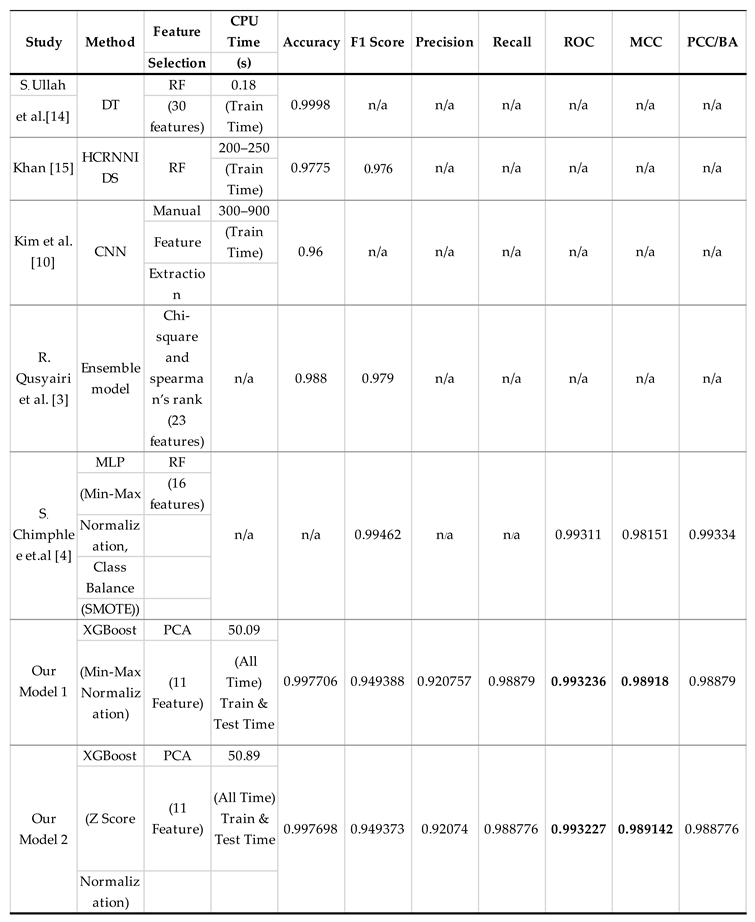
The Table 5 compares various models to the CSE-CIC-IDS-2018 dataset, measuring their accuracy, training time, and other performance measures. S. Ullah et al. [14] employed a Decision Tree (DT) with random feature selection (30 features) to achieve an astounding 0.9998 accuracy in a very low training period (0.18 seconds). Khan [15] Used random feature selection to implement an HCRNNIDS model, obtaining 0.9775 accuracy in 200-250 seconds. F1 score and precision values were not specified. Kim et al. [10] Convolutional Neural Network (CNN) with manual feature extraction was used. In a training duration ranging from 300 to 900 seconds, I achieved an accuracy of 0.960. F1 score, precision, and recall measures were not provided in detail. R. Qusyairi et al. [3] Applied an ensemble model with 23 randomly chosen features. Although the accuracy was 0.988, no precise F1 score, precision, or recall statistics were provided. S. Chimphlee et al. [4] used Min-Max normalization, Random Forest feature selection, and Class Balance (SMOTE), as well as Multi-Layer Perceptron (MLP). A high accuracy of 0.99462 was achieved, with significant precision and recall values.
Our Model 1 and Model 2: Both models used XGBoost with Principal Component Analysis (PCA) to pick features. Our Model 1 was 0.997706 accurate, while our Model 2 was 0.997698 accurate. Both models performed well across multiple parameters, including F1 score, precision, recall, ROC, and MCC.In conclusion, the proposed models demonstrate a variety of approaches, with PCA being particularly helpful in lowering feature dimensions while maintaining high accuracy. The models yield remarkable results in intrusion detection, reflecting the ongoing progress in the field of machine learning applied to cybersecurity.
6. Conclusions
After examining the data, it was discovered that three models, namely XGBoost, DT, and RF, had remarkable performance in terms of both ROC values and CPU runtime. As a result, these models were evaluated further in conjunction with feature selection techniques combining PCA and RF. Finally, the combination of XGBoost for classification and feature selection with PCA, resulting in 11 features, produced the best ROC and CPU runtime values. Interestingly, the usefulness of these values remained consistent regardless of whether normalization approaches such as min-max or z-score were used; the changes seen were not significant. Machine learning classification techniques, as is widely accepted, can be used to assess and anticipate infiltrations. The algorithm performed admirably after preprocessing tactics and feature selection approaches were applied. Although this strategy outperformed others, its utility may be limited in some cases. We argue that the trained models are not yet ready for use in real-world scenarios. Existing models must be improved, and new algorithms developed to address the issues given by unbalanced datasets. Furthermore, dynamic testing with multiple types of infiltration is required. In the future, we intend to examine the impact of deep learning on increasing time complexity and model size, consequently boosting the efficiency of network intrusion detection in real-time settings.
Author Contributions
s. Songma; Conceptualization, Methodology, Data curation, Software, Writing original draft, Investigation, Validation and Visualization; T. Sathuphan; Supervision, Formal Analysis, Resources, Writing review and editing, Validation, and Investigation. T. Pamutha; Writing original draft, Writing review and editing, Validation, and Visualization. All authors have read and agreed to the published version of the manuscript.
Funding
This research received no external funding.
Institutional Review Board Statement
Not applicable.
Informed Consent Statement
Not applicable.
Data Availability Statement
The CSE-CIC-IDS-2018 dataset used in the research is available at the following link: https://registry.opendata.aws/cse-cic-ids2018/.
Conflicts of Interest
The authors declare no conflicts of interest.
References
- A. Momand, S. U. Jan, and N. Ramzan, “A Systematic and Comprehensive Survey of Recent Advances in Intrusion Detection Systems Using Machine Learning: Deep Learning, Datasets, and Attack Taxonomy,” Journal of Sensors, vol. 2023. Hindawi Limited, 2023. [CrossRef]
- M. Aljanabi, M. A. Ismail, and A. H. Ali, “Intrusion detection systems, issues, challenges, and needs,” International Journal of Computational Intelligence Systems, vol. 14, no. 1, pp. 560–571, 2021. [CrossRef]
- R. Qusyairi, F. Saeful, and R. Kalamullah, “Implementation of Ensemble Learning and Feature Selection for Performance Improvements in Anomaly-Based Intrusion Detection Systems,” International Conference on Industry 4.0, Artificial Intelligence, and Communications Technology (IAICT), 2020. Accessed: Oct. 23, 2023. [Online]. Available: IEEE.
- S. Chimphlee and W. Chimphlee, “Machine learning to improve the performance of anomaly-based network intrusion detection in big data,” Indonesian Journal of Electrical Engineering and Computer Science, vol. 30, no. 2, pp. 1106–1119, May 2023. [CrossRef]
- N. Kaja, A. Shaout, and D. Ma, “An intelligent intrusion detection system,” Applied Intelligence, vol. 49, no. 9, pp. 3235–3247, Sep. 2019. [CrossRef]
- C. Z. Mubarak Albarka Umar, “Effects of Feature Selection and Normalization on Network Effects of Feature Selection and Normalization on Network Intrusion Detection Intrusion Detection,” Umar, Mubarak Albarka; Zhanfang, Chen (2020): Effects of Feature Selection and Normalization on Network Intrusion Detection. TechRxiv. Preprint. [CrossRef]
- A. S. Jaradat, M. M. Barhoush, and R. B. Easa, “Network intrusion detection system: Machine learning approach,” Indonesian Journal of Electrical Engineering and Computer Science, vol. 25, no. 2, pp. 1151–1158, Feb. 2022. [CrossRef]
- Institute of Electrical and Electronics Engineers, “An Ensemble Approach for Intrusion Detection System Using Machine Learning Algorithms”.
- A. B. Nassif, M. A. Talib, Q. Nasir, and F. M. Dakalbab, “Machine Learning for Anomaly Detection: A Systematic Review,” IEEE Access, vol. 9. Institute of Electrical and Electronics Engineers Inc., pp. 78658–78700, 2021. [CrossRef]
- J. Kim, Y. Shin, and E. Choi, “An Intrusion Detection Model based on a Convolutional Neural Network,” Journal of Multimedia Information System, vol. 6, no. 4, pp. 165–172, Dec. 2019. [CrossRef]
- G. Karatas, O. Demir, and O. K. Sahingoz, “Increasing the Performance of Machine Learning-Based IDSs on an Imbalanced and Up-to-Date Dataset,” IEEE Access, vol. 8, pp. 32150–32162, 2020. [CrossRef]
- M. A. Ambusaidi, X. He, P. Nanda, and Z. Tan, “Building an intrusion detection system using a filter-based feature selection algorithm,” IEEE Transactions on Computers, vol. 65, no. 10, pp. 2986–2998, Oct. 2016. [CrossRef]
- A. R. Muhsen, G. G. Jumaa, N. F. A. Bakri, and A. T. Sadiq, “Feature Selection Strategy for Network Intrusion Detection System (NIDS) Using Meerkat Clan Algorithm,” International Journal of Interactive Mobile Technologies, vol. 15, no. 16, pp. 158–171, 2021. [CrossRef]
- S. Ullah, Z. Mahmood, N. Ali, T. Ahmad, and A. Buriro, “Machine Learning-Based Dynamic Attribute Selection Technique for DDoS Attack Classification in IoT Networks,” Computers, vol. 12, no. 6, Jun. 2023. [CrossRef]
- M. A. Khan, “HCRNNIDS: Hybrid convolutional recurrent neural network-based network intrusion detection system,” Processes, vol. 9, no. 5, 2021. [CrossRef]
- J. L. Leevy and T. M. Khoshgoftaar, “A survey and analysis of intrusion detection models based on CSE-CIC-IDS2018 Big Data,” J Big Data, vol. 7, no. 1, Dec. 2020. [CrossRef]
- Sri Venkateshwara College of Engineering. Department of Electronics and Communication Engineering, Institute of Electrical and Electronics Engineers. Bangalore Section, Institute of Electrical and Electronics Engineers. Bangalore Section. COM Chapter, Sri Venkateshwara College of Engineering, and Institute of Electrical and Electronics Engineers, “Principle Component Analysis based Intrusion”.
- Md. A. M. Hasan, M. Nasser, S. Ahmad, and K. I. Molla, “Feature Selection for Intrusion Detection Using Random Forest,” Journal of Information Security, vol. 07, no. 03, pp. 129–140, 2016. [CrossRef]
- S. S. Dhaliwal, A. Al Nahid, and R. Abbas, “Effective intrusion detection system using XGBoost,” Information (Switzerland), vol. 9, no. 7, Jun. 2018. [CrossRef]
- Institute of Electrical and Electronics Engineers, “An Anomaly-Based Intrusion Detection System for the Smart Grid Based on CART Decision Tree”.
- S. Shilpashree, S. C. Lingareddy, N. G. Bhat, and G. Sunil Kumar, “Decision tree: A machine learning for intrusion detection,” International Journal of Innovative Technology and Exploring Engineering, vol. 8, no. 6 Special Issue 4, pp. 1126–1130, Apr. 2019. [CrossRef]
- R. Wazirali, “An Improved Intrusion Detection System Based on KNN Hyperparameter Tuning and Cross-Validation,” Arab J Sci Eng, vol. 45, no. 12, pp. 10859–10873, Dec. 2020. [CrossRef]
- E. Jamal, M. Reza, and G. Jamal, “Intrusion Detection System Based on Multi-Layer Perceptron Neural Networks and Decision Tree,” in International Conference on Information and Knowledge Technology, 2015.
- N. Farnaaz and M. A. Jabbar, “Random Forest Modeling for Network Intrusion Detection System,” in Procedia Computer Science, Elsevier B.V., 2016, pp. 213–217. [CrossRef]
- Academy of Technology and Institute of Electrical and Electronics Engineers, “Proposed GA-BFSS and Logistic Regression based Intrusion Detection System”.
- IEEE Women in Engineering Committee, Institute of Electrical and Electronics Engineers. Bangalore Section. Women in Engineering Affinity Group, W. in E. A. Group. Institute of Electrical and Electronics Engineers. Bangladesh Section, Defence Research & Development Organisation (India), and Institute of Electrical and Electronics Engineers, Intrusion Detection System using Naive Bayes algorithm.
- W. Li and Z. Liu, “A method of SVM with normalization in intrusion detection,” in Procedia Environmental Sciences, Elsevier B.V., 2011, pp. 256–262. [CrossRef]
- G. Ketepalli and P. Bulla, “Data Preparation and Pre-processing of Intrusion Detection Datasets using Machine Learning,” in 6th International Conference on Inventive Computation Technologies, ICICT 2023—Proceedings, Institute of Electrical and Electronics Engineers Inc., 2023, pp. 257–262. [CrossRef]
- ICT Research Institute, Institute of Electrical and Electronics Engineers, Institute of Electrical and Electronics Engineers. Iran Section., Iran. Vizarat-i Irtibatat va Fanavari-i Ittilaat., and Iranian Association of Electrical and Electronics Engineers., Intrusion Detection Based on MinMax K-means Clustering.
- Z. Zeng, W. Peng, and B. Zhao, “Improving the Accuracy of Network Intrusion Detection with Causal Machine Learning,” Security and Communication Networks, vol. 2021, 2021. [CrossRef]
- T. T. H. Le, H. Kim, H. Kang, and H. Kim, “Classification and Explanation for Intrusion Detection System Based on Ensemble Trees and SHAP Method,” Sensors, vol. 22, no. 3, Feb. 2022. [CrossRef]
- D. Chicco and G. Jurman, “The advantages of the Matthews correlation coefficient (MCC) over F1 score and accuracy in binary classification evaluation,” BMC Genomics, vol. 21, no. 1, Jan. 2020. [CrossRef]
- M. Sarhan, S. Layeghy, N. Moustafa, M. Gallagher, and M. Portmann, “Feature extraction for machine learning-based intrusion detection in IoT networks,” Digital Communications and Networks, Sep. 2022. [CrossRef]
Figure 1.
This proposed framework.
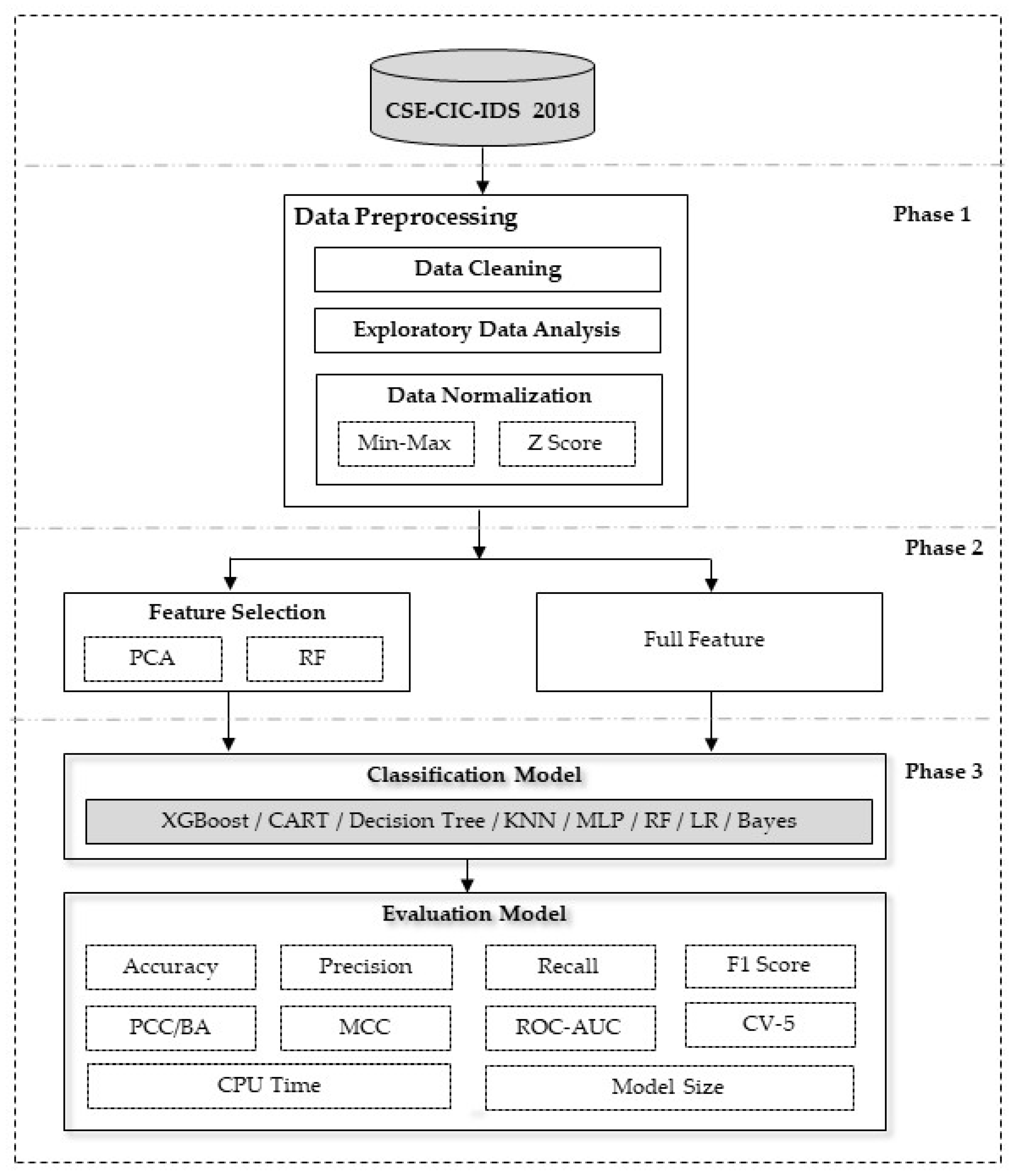
Figure 2.
Network traffic distribution.
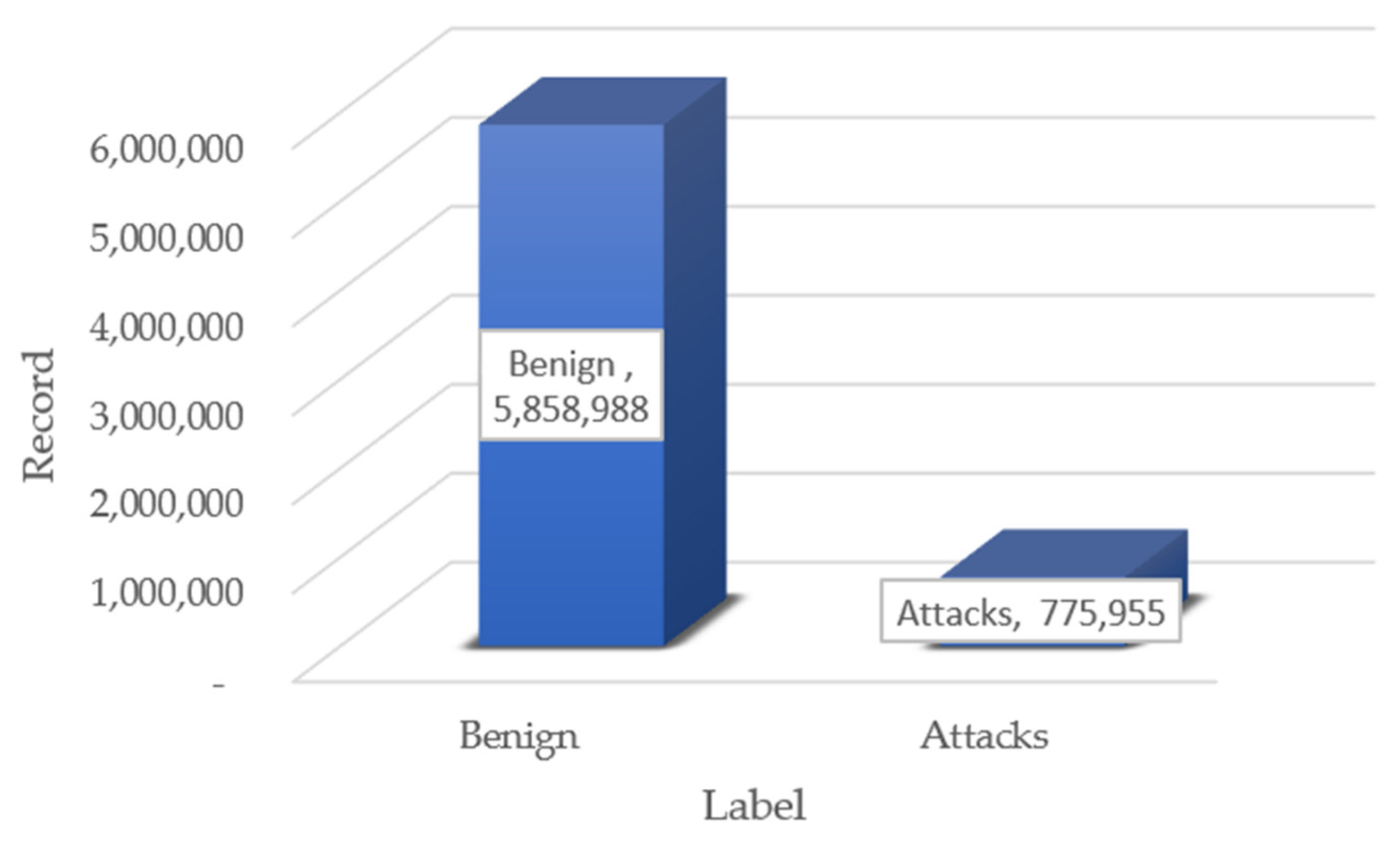
Figure 3.
Feature selection by using PCA considering variance ratios.
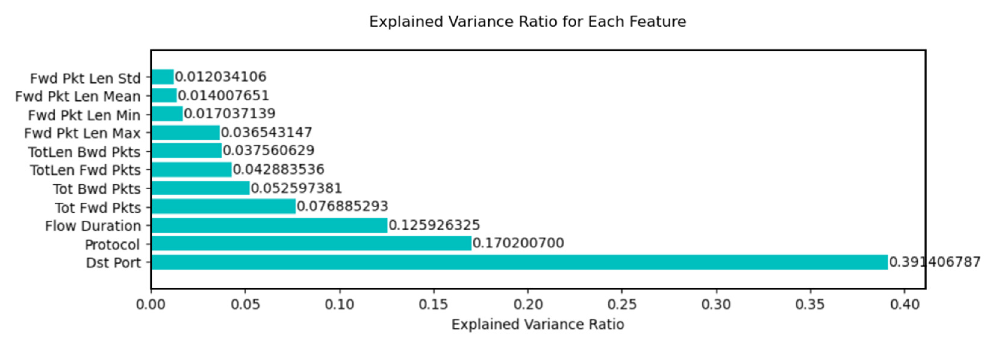
Figure 4.
Feature selection by using RF considering variance ratios.
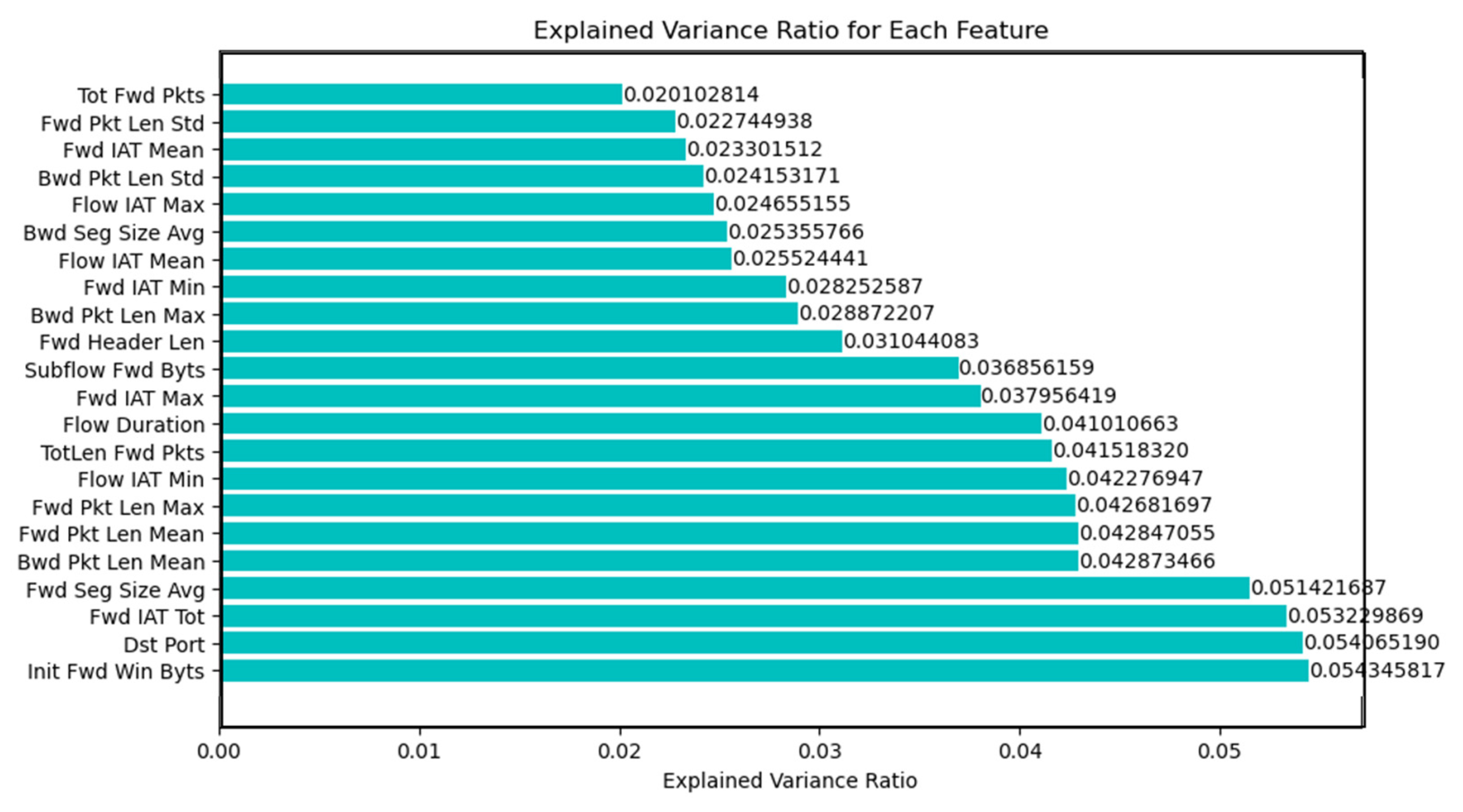
Figure 5.
Radar Chart for Classification Performance with Feature Selection and Min-Max Normalization.
Figure 5.
Radar Chart for Classification Performance with Feature Selection and Min-Max Normalization.
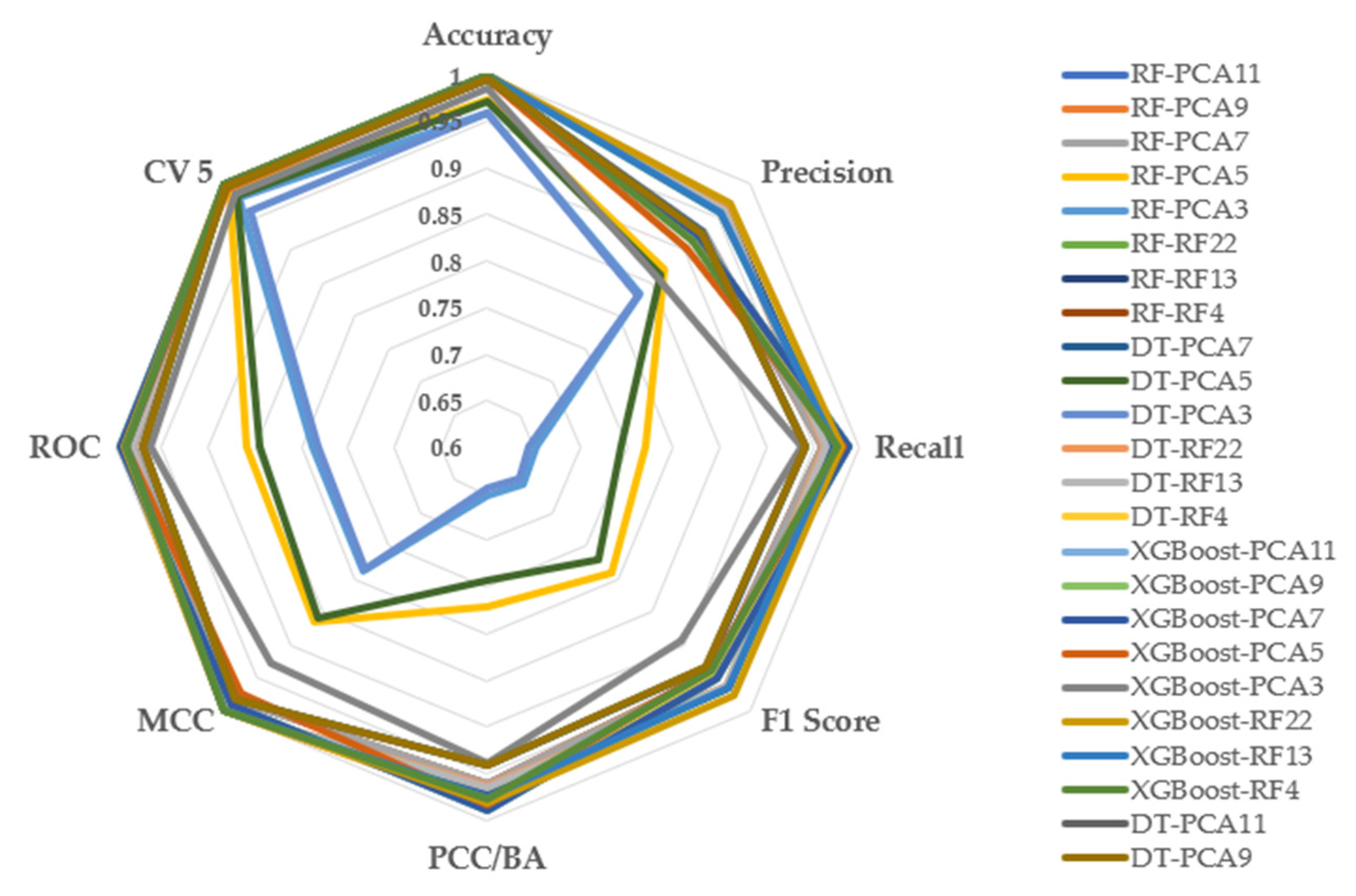
Figure 6.
Radar Chart for Classification Performance with Feature Selection and Z Score Normalization.
Figure 6.
Radar Chart for Classification Performance with Feature Selection and Z Score Normalization.
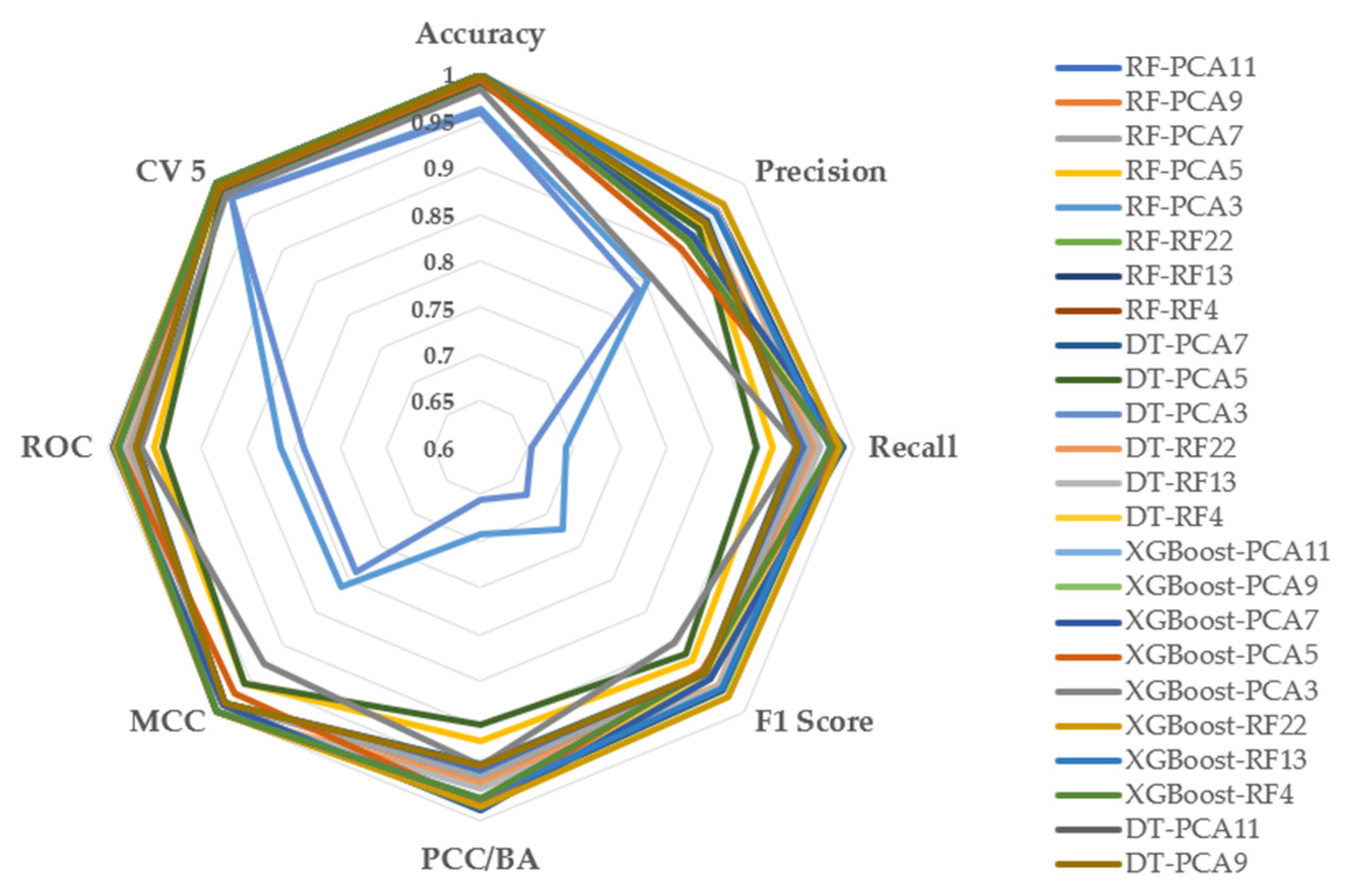

Table 1.
The Effect of Data Cleaning on Attack Category Distribution.
| Type | Original Data | After Clean Data | ||
|---|---|---|---|---|
| Label Feature | Record | Percent | Record | Percent |
| Benign | 7,733,390 | 85.95 | 5,858,988 | 88.31 |
| DoS attacks-LOIC-HTTP | 576,191 | 6.40 | 575,364 | 8.67 |
| DDOS attack-HOIC | 686,012 | 7.62 | 198,861 | 3.00 |
| DDOS attack-LOIC-UDP | 1,730 | 0.02 | 1,730 | 0.03 |
| total | 8,997,323 | 100.00 | 6,634,943 | 100.00 |
Table 2.
Summary of Classifier Performance Metrics using Min-Max and Z Score Normalization.
| Classifiers | Accuracy | Precision | Recall | F1 Score | PCC/BA | MCC | ROC | CV 5 | CPU Time (S) |
Model Size (KB) |
|---|---|---|---|---|---|---|---|---|---|---|
| Min-Max | ||||||||||
| XGBoost | 0.999950 | 0.975427 | 0.982578 | 0.978946 | 0.982578 | 0.999765 | 0.991281 | 0.999930 | 92.86 | 590.85 |
| CART | 0.999917 | 0.967775 | 0.960877 | 0.964270 | 0.960877 | 0.999609 | 0.980424 | 0.997995 | 112.79 | 57.31 |
| DT | 0.999911 | 0.958447 | 0.960853 | 0.959643 | 0.960853 | 0.999580 | 0.980413 | 0.999889 | 65.41 | 68.74 |
| RF | 0.999631 | 0.956304 | 0.982593 | 0.968626 | 0.982593 | 0.998260 | 0.991064 | 0.999560 | 131.67 | 7,860.20 |
| Bayes | 0.950489 | 0.747992 | 0.984988 | 0.831505 | 0.984988 | 0.820660 | 0.986005 | 0.950566 | 7.02 | 6.65 |
| LR | 0.992956 | 0.898140 | 0.989497 | 0.937082 | 0.989497 | 0.967303 | 0.992159 | 0.989964 | 860.09 | 4.58 |
| MLP | 0.999835 | 0.938870 | 0.993869 | 0.962856 | 0.993869 | 0.999221 | 0.996879 | 0.998905 | 2,220.53 | 291.93 |
| KNN | 0.999848 | 0.947640 | 0.963627 | 0.955322 | 0.963627 | 0.999281 | 0.981772 | 0.999815 | 6,460.54 | 2,861,321.35 |
| Z Score | ||||||||||
| XGBoost | 0.999948 | 0.977524 | 0.977526 | 0.977525 | 0.977526 | 0.999755 | 0.988754 | 0.999934 | 89.12 | 581.15 |
| CART | 0.999921 | 0.968903 | 0.964489 | 0.966674 | 0.964489 | 0.999626 | 0.982229 | 0.997749 | 151.42 | 56.89 |
| DT | 0.999918 | 0.960671 | 0.967360 | 0.963963 | 0.967360 | 0.999612 | 0.983669 | 0.999881 | 76.50 | 68.93 |
| RF | 0.999739 | 0.966118 | 0.982353 | 0.973918 | 0.982353 | 0.998769 | 0.991008 | 0.999603 | 153.25 | 17,055.20 |
| Bayes | 0.949471 | 0.752121 | 0.984739 | 0.834724 | 0.984739 | 0.817708 | 0.985739 | 0.950838 | 7.43 | 6.65 |
| LR | 0.996893 | 0.912855 | 0.994199 | 0.947252 | 0.994199 | 0.985584 | 0.996643 | 0.995351 | 6920.85 | 4.58 |
| MLP | 0.998974 | 0.923494 | 0.998375 | 0.954336 | 0.998375 | 0.995160 | 0.998676 | 0.998805 | 1167.41 | 291.81 |
| KNN | 0.999840 | 0.945759 | 0.967207 | 0.955923 | 0.967207 | 0.999246 | 0.983554 | 0.999803 | 11,468.02 | 2,861,321.35 |
Table 3.
A Comparison of Classifier Performance with Different Feature Selection and Normalization Techniques.
Table 3.
A Comparison of Classifier Performance with Different Feature Selection and Normalization Techniques.
| Classifiers | Accuracy | Precision | Recall | F1 Score | PCC/BA | MCC | ROC | CV 5 | CPU Time (S) |
Model Size (KB) |
|---|---|---|---|---|---|---|---|---|---|---|
| Min-Max | ||||||||||
| RF-PCA11 | 0.996154 | 0.925325 | 0.960638 | 0.942236 | 0.960638 | 0.982109 | 0.979327 | 0.997329 | 135.52 | 31,307.31 |
| RF-PCA9 | 0.996145 | 0.926899 | 0.960586 | 0.943059 | 0.960586 | 0.982067 | 0.979291 | 0.997325 | 131.46 | 31,335.76 |
| RF-PCA7 | 0.996159 | 0.927997 | 0.960655 | 0.943677 | 0.960655 | 0.982134 | 0.979337 | 0.997324 | 137.16 | 31,305.15 |
| RF-PCA5 | 0.972420 | 0.869089 | 0.770071 | 0.789002 | 0.770071 | 0.863637 | 0.859193 | 0.991191 | 168.64 | 55,616.56 |
| RF-PCA3 | 0.958392 | 0.832067 | 0.652148 | 0.655230 | 0.652148 | 0.788547 | 0.787589 | 0.977432 | 197.05 | 334,645.57 |
| RF-RF22 | 0.999870 | 0.955205 | 0.975940 | 0.965073 | 0.975940 | 0.999385 | 0.987934 | 0.999761 | 188.84 | 10,281.29 |
| RF-RF13 | 0.999920 | 0.960641 | 0.970969 | 0.965681 | 0.970969 | 0.999623 | 0.985472 | 0.999881 | 154.06 | 5,400.85 |
| RF-RF4 | 0.999837 | 0.913762 | 0.983025 | 0.942297 | 0.983025 | 0.999232 | 0.991467 | 0.999819 | 129.30 | 1,241.54 |
| DT-PCA11 | 0.996097 | 0.925248 | 0.940889 | 0.932627 | 0.940889 | 0.981836 | 0.969390 | 0.997278 | 8.67 | 1,173.92 |
| DT-PCA9 | 0.996098 | 0.925831 | 0.940891 | 0.932914 | 0.940891 | 0.981840 | 0.969392 | 0.997278 | 6.77 | 1,174.43 |
| DT-PCA7 | 0.996099 | 0.925985 | 0.941614 | 0.933358 | 0.941614 | 0.981843 | 0.969753 | 0.997283 | 6.20 | 1,174.20 |
| DT-PCA5 | 0.971348 | 0.861854 | 0.743431 | 0.769738 | 0.743431 | 0.858021 | 0.844684 | 0.981260 | 5.35 | 2,028.59 |
| DT-PCA3 | 0.957864 | 0.829175 | 0.643716 | 0.647520 | 0.643716 | 0.785412 | 0.782492 | 0.959822 | 5.95 | 12,713.26 |
| DT-RF22 | 0.999918 | 0.961201 | 0.963030 | 0.962111 | 0.963030 | 0.999612 | 0.981504 | 0.999884 | 40.10 | 83.07 |
| DT-RF13 | 0.999916 | 0.960222 | 0.964468 | 0.962324 | 0.964468 | 0.999602 | 0.982222 | 0.999882 | 25.03 | 84.21 |
| DT-RF4 | 0.999836 | 0.913430 | 0.983022 | 0.942066 | 0.983022 | 0.999224 | 0.991465 | 0.999816 | 5.47 | 42.21 |
| XGBoost-PCA11 | 0.997706 | 0.920757 | 0.988790 | 0.949388 | 0.988790 | 0.989180 | 0.993236 | 0.997635 | 50.74 | 660.01 |
| XGBoost-PCA9 | 0.997705 | 0.920756 | 0.988784 | 0.949385 | 0.988784 | 0.989177 | 0.993233 | 0.997634 | 46.13 | 667.18 |
| XGBoost-PCA7 | 0.997705 | 0.920752 | 0.988784 | 0.949383 | 0.988784 | 0.989177 | 0.993233 | 0.997631 | 44.52 | 661.26 |
| XGBoost-PCA5 | 0.994354 | 0.902693 | 0.982245 | 0.936947 | 0.982245 | 0.973601 | 0.988806 | 0.994281 | 45.00 | 787.88 |
| XGBoost-PCA3 | 0.984300 | 0.858634 | 0.938125 | 0.893717 | 0.938125 | 0.927370 | 0.961847 | 0.983735 | 44.21 | 741.86 |
| XGBoost-RF22 | 0.999940 | 0.969710 | 0.981110 | 0.975265 | 0.981110 | 0.999719 | 0.990545 | 0.999933 | 54.15 | 572.66 |
| XGBoost-RF13 | 0.999917 | 0.956144 | 0.974560 | 0.964956 | 0.974560 | 0.999609 | 0.987267 | 0.999916 | 44.84 | 573.72 |
| XGBoost-RF4 | 0.999812 | 0.912773 | 0.976517 | 0.939387 | 0.976517 | 0.999111 | 0.988202 | 0.999809 | 40.56 | 564.10 |
| Z Score | ||||||||||
| RF-PCA11 | 0.997387 | 0.939662 | 0.948200 | 0.943840 | 0.948200 | 0.987658 | 0.972616 | 0.997016 | 139.92 | 40,746.06 |
| RF-PCA9 | 0.997396 | 0.940383 | 0.955569 | 0.947705 | 0.955569 | 0.987658 | 0.976323 | 0.996991 | 145.87 | 40,614.20 |
| RF-PCA7 | 0.997396 | 0.939566 | 0.953297 | 0.946201 | 0.953297 | 0.987702 | 0.975172 | 0.997000 | 143.99 | 40,533.90 |
| RF-PCA5 | 0.991311 | 0.933681 | 0.913607 | 0.922487 | 0.913607 | 0.958517 | 0.949896 | 0.991049 | 183.93 | 69,791.18 |
| RF-PCA3 | 0.962557 | 0.854850 | 0.692485 | 0.724899 | 0.692485 | 0.812001 | 0.813312 | 0.978074 | 222.77 | 353,408.88 |
| RF-RF22 | 0.999882 | 0.958170 | 0.977381 | 0.967350 | 0.977381 | 0.999441 | 0.988660 | 0.999794 | 202.37 | 12,587.54 |
| RF-RF13 | 0.999918 | 0.957692 | 0.977453 | 0.967121 | 0.977453 | 0.999612 | 0.988714 | 0.999879 | 192.22 | 5,940.48 |
| RF-RF4 | 0.999837 | 0.913762 | 0.983025 | 0.942297 | 0.983025 | 0.999232 | 0.991467 | 0.999817 | 130.35 | 1,221.85 |
| DT-PCA11 | 0.997312 | 0.941784 | 0.940745 | 0.941254 | 0.940745 | 0.987290 | 0.968679 | 0.996832 | 9.58 | 1,290.92 |
| DT-PCA9 | 0.997311 | 0.941636 | 0.940022 | 0.940820 | 0.940022 | 0.987286 | 0.968317 | 0.996831 | 7.39 | 1,289.56 |
| DT-PCA7 | 0.997311 | 0.942492 | 0.938582 | 0.940528 | 0.938582 | 0.987286 | 0.967597 | 0.996835 | 6.65 | 1,289.70 |
| DT-PCA5 | 0.990910 | 0.931768 | 0.896305 | 0.912423 | 0.896305 | 0.956527 | 0.940553 | 0.990634 | 5.99 | 2,385.40 |
| DT-PCA3 | 0.958382 | 0.839611 | 0.655594 | 0.670713 | 0.655594 | 0.788676 | 0.789885 | 0.977744 | 6.86 | 13,686.38 |
| DT-RF22 | 0.999913 | 0.959644 | 0.960858 | 0.960249 | 0.960858 | 0.999591 | 0.980417 | 0.999889 | 45.22 | 84.20 |
| DT-RF13 | 0.999916 | 0.959630 | 0.964470 | 0.962023 | 0.964470 | 0.999605 | 0.982224 | 0.999882 | 29.13 | 82.90 |
| DT-RF4 | 0.999836 | 0.913430 | 0.983022 | 0.942066 | 0.983022 | 0.999224 | 0.991465 | 0.999816 | 6.44 | 41.84 |
| XGBoost-PCA11 | 0.997698 | 0.920740 | 0.988776 | 0.949373 | 0.988776 | 0.989142 | 0.993227 | 0.997635 | 50.89 | 667.12 |
| XGBoost-PCA9 | 0.997693 | 0.920721 | 0.988770 | 0.949360 | 0.988770 | 0.989117 | 0.993225 | 0.997634 | 45.37 | 668.91 |
| XGBoost-PCA7 | 0.997697 | 0.920736 | 0.988770 | 0.949367 | 0.988770 | 0.989138 | 0.993223 | 0.997633 | 42.65 | 673.14 |
| XGBoost-PCA5 | 0.994341 | 0.902696 | 0.982201 | 0.936926 | 0.982201 | 0.973534 | 0.988765 | 0.994289 | 42.59 | 784.36 |
| XGBoost-PCA3 | 0.984288 | 0.858767 | 0.939827 | 0.894489 | 0.939827 | 0.927392 | 0.962789 | 0.983736 | 42.28 | 732.69 |
| XGBoost-RF22 | 0.999943 | 0.968946 | 0.984719 | 0.976556 | 0.984719 | 0.999733 | 0.992350 | 0.999935 | 52.72 | 573.66 |
| XGBoost-RF13 | 0.999918 | 0.956262 | 0.975282 | 0.965350 | 0.975282 | 0.999612 | 0.987628 | 0.999916 | 44.31 | 573.12 |
| XGBoost-RF4 | 0.999812 | 0.912765 | 0.976521 | 0.939385 | 0.976521 | 0.999111 | 0.988207 | 0.999809 | 40.07 | 563.23 |
Table 4.
List Feature and Importance score with PCA11.
| Feature Name | Importance Score |
|---|---|
| Dst Port | 0.391406787 |
| Protocol | 0.170200700 |
| Flow Duration | 0.125926325 |
| Tot Fwd Pkts | 0.076885293 |
| Tot Bwd Pkts | 0.052597381 |
| TotLen Fwd Pkts | 0.042883536 |
| TotLen Bwd Pkts | 0.037560629 |
| Fwd Pkt Len Max | 0.036543147 |
| Fwd Pkt Len Min | 0.017037139 |
| Fwd Pkt Len Mean | 0.014007651 |
| Fwd Pkt Len Std | 0.012034106 |
Table 5.
Comparison of Intrusion Detection Models Using the CSE-CIC-IDS-2018 Dataset.
 |
Disclaimer/Publisher’s Note: The statements, opinions and data contained in all publications are solely those of the individual author(s) and contributor(s) and not of MDPI and/or the editor(s). MDPI and/or the editor(s) disclaim responsibility for any injury to people or property resulting from any ideas, methods, instructions or products referred to in the content. |
© 2023 by the authors. Licensee MDPI, Basel, Switzerland. This article is an open access article distributed under the terms and conditions of the Creative Commons Attribution (CC BY) license (http://creativecommons.org/licenses/by/4.0/).
Copyright: This open access article is published under a Creative Commons CC BY 4.0 license, which permit the free download, distribution, and reuse, provided that the author and preprint are cited in any reuse.


