Preprint

Article

Optimal Control Law for the Flutter Suppression of a Wing Section in Compressible Flows

Altmetrics

Downloads

Views

Comments

Álvaro Muñoz,

Pablo García-Fogeda^*

Álvaro Muñoz,

Pablo García-Fogeda^*

This version is not peer-reviewed

Submitted:

03 November 2023

Posted:

06 November 2023

You are already at the latest version

Alerts

Abstract

This paper presents various procedures for determining the optimal control law for a wing section in compressible flow. The flow regime includes subsonic as well as supersonic flows. For the evolution of the system in the Laplace plane the present method makes use of the exact unsteady aerodynamic forces in the Laplace plane once the control law is established. This is a great advantage against other results previously published, where the unsteady aerodynamics in the Laplace plane are just approximations of the curve-fitted values in the frequency domain (imaginary axis). Different control techniques are investigated like pole-placement, LQR and H-infinity norm. Among these, the H-infinity norm emerges as the optimal choice, exhibiting a norm magnitude approximately two orders of magnitude lower than the LQR case. Furthermore, the H-infinity controller demonstrates lower pole values that those of the pole placement and LQR compensator, showing the advantage of the H-infinity controller in terms of economic efficiency.

Keywords:

Subject: Engineering - Aerospace Engineering

1. Introduction

New high-aspect-ratio lightweight wings development is now the main objective in aviation, with the objective of reducing fuel consumption and to diminish greenhouse gas emissions. However, these advanced wings are more susceptible to aeroelastic instabilities, such as flutter or divergence. A solution to overcome such instabilities is the implementation of active control on the wing structure thus extending its flight envelope. Active flutter suppression (AFS) has been known for some time, see for example [1] and [2]. Despite its potential, the practical implementation of AFS faces several challenges. These include the need for a robust method to compute unsteady aerodynamics valid in the Laplace domain, devising a control law that remains effective across the full compressible regime, and determining an optimal control strategy capable of minimizing energy consumption.

As mentioned by Livne [3], for any AFS solution to be accepted it must be fully understood and supported by reliable tools. Consequently, there exists a pressing need for a practical and robust AFS system suitable for integration into aircraft systems. For multi-input-output systems, AFS often requires many trial designs before achieving satisfactory results. Modern state-space control design methods seem more compatible with general multi-input-output systems, and many techniques like linear quadratic Gaussian (LQG) [4],

H_{\infty}

control [5,6], or pole and partial or complete eigenstructures assignment [7,8] have proven their validity for applications with multiple-input multiple-output systems. However, when applied to active-flutter suppression, these methods suffer from the need of greatly augmenting the states of the model in order to express the generalized aerodynamic forces matrix in the state space. These additional states are fictitious, unmeasurable, and very sensitive to the modeling approximation inherent in the aerodynamic formulation used.

Linear Matrix Inequalities (LMIs) have proven to derive suboptimal designs for linear control problems [9]. Chiali and Gahinet [10] extended the LMI approach to multi-objective output feedback synthesis. Gahinet and Apkarian [11] used LMI and extended the concept of

H_{\infty}

controllers replacing the Ricatti equations by Ricatti inequalities to parameterize the suboptimal

H_{\infty}

controllers, including reduced-order variants.

In this study, we focus on the implementation of AFS for a wing section with three degrees of freedom, within the full compressible regime. The aerodynamics in the Laplace domain presented at [12] will be used, and different procedures to determine the optimal control law will be investigated. It will be shown that the

H_{\infty}

controllers provide the best result in terms of stability for all the cases presented.

The paper’s organization is as follows: Section 2 presents the equations of motion for the state-space model, Section 3 delves into the development of the standard compensator for system stabilization, Section 4 introduces the

H_{\infty}

controller and discusses its internal stability, Section 5 presents the results obtained in compressible regime and Section 6 offers the concluding remarks for this work.

2. Equations of motion and State-Space modelization

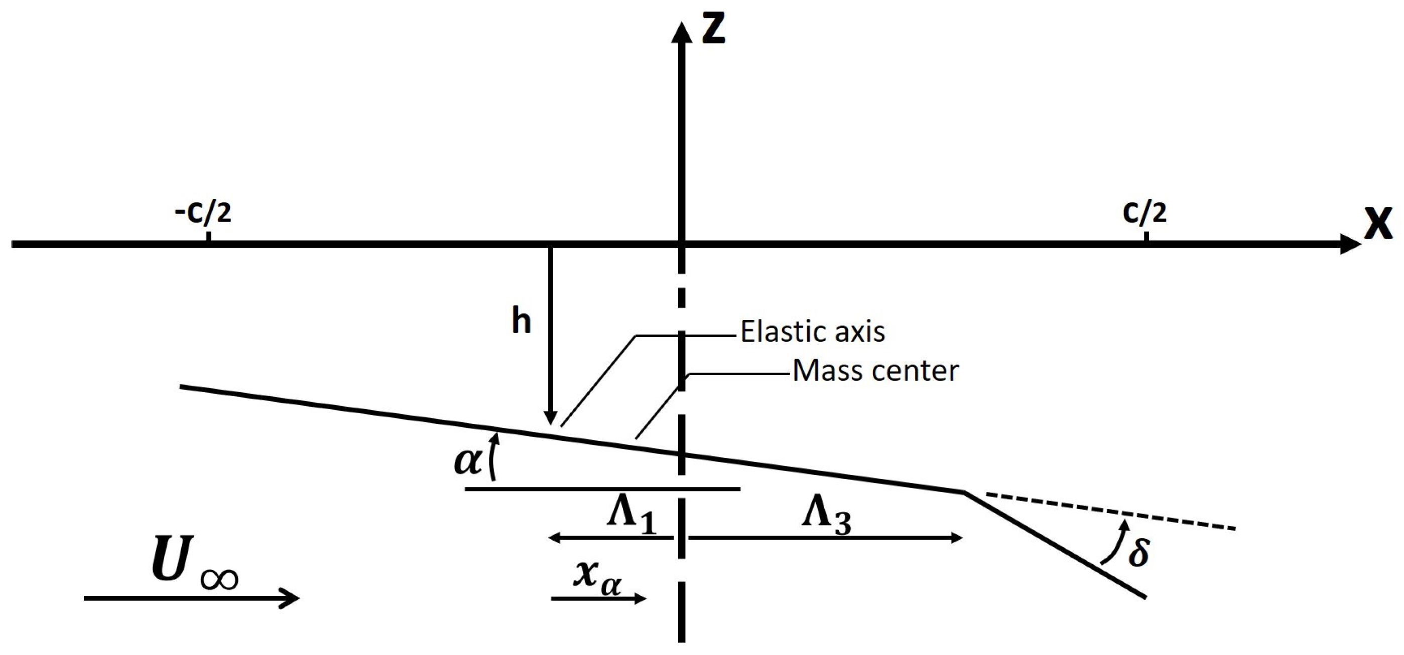
This paper deals with the control of a three degrees of freedom airfoil (Figure 1) in compressible regime. The dynamics of such plant is taken from [12], as well as the analytic expressions for the unsteady aerodynamic loads. The dynamic equation of the system in the Laplace domain is:

(M_{s} p^{2} + B_{s} p + K_{s}) x_{q} = \frac{η}{2} {(\frac{U}{b})}^{2} Q (\frac{p b}{U}) x_{q} + G u

(1)

where

η = \frac{1}{π μ}

μ

is the non-dimensional mass ratio,

{x_{q}} = {[\frac{h}{b} α δ]}^{T}

is the state of the plant,

Q (\frac{p b}{U})

the unsteady aerodynamic loads and u the external moment applied to the control surface. Matrices

M_{s}

B_{s}

K_{s}

and G can be obtained directly from Edwards[13].

Introducing the non-dimensional Laplace variable,

s = \frac{p b}{U}

Equation 1 is expressed as:

(M_{s} {(\frac{U}{b})}^{2} s^{2} + B_{s} (\frac{U}{b}) s + K_{s} - \frac{η}{2} {(\frac{U}{b})}^{2} Q (s)) x_{q} = G u

(2)

In order to manipulate the system and to obtain an adequate control law, the system’s equations of motion must be transformed to the state-space. For the control law evaluation, a Rational Function Approximation (RFA) methodology will be employed, following Roger´s model[14]. It must be noted that the use of RFAs introduces inherent inaccuracies in the model, since the data fitting may not be exact. Therefore, the RFA will only be used to compute the control law, and the exact dynamic equation will be applied when presenting the resulting behaviour in a closed-loop configuration, being this one of the main advantages of the proposed method in this work.

This Roger´s approximation contains a number of common lags, representing the aerodynamic lag of the system and is expressed as:

Q (s) = - A_{0} - A_{1} s - A_{2} s^{2} - \sum_{j = 3}^{N} \frac{A_{j} s}{s + γ_{j - 2}}

(3)

As the model’s order exhibits linear growth in correspondence to the number of lags, it is not advisable to select a high number of lag states. Typically,

N = 6

is enough for most applications, as suggested by Karpel[2]. When represented in matrix form, this RFA can be conveniently expressed as:

Q (s) = - A_{0} - A_{1} s - A_{2} s^{2} - D {(s I - R)}^{- 1} E s

(4)

where R contains the lags of the system and D acts as a summation matrix.

To determine the matrices

A_{0}

A_{1}

A_{2}

, and E, one must provide an adequate number of generalized aerodynamic force matrices to fit the model. A conventional approach involves computing these loads under the assumption of simple harmonic oscillations, i.e. pure imaginary reduced frequencies. However, by incorporating data from across the Laplace plane, the model is expected to increase its accuracy far from the imaginary axis. These aerodynamic loads serve as the foundation for fitting the model through the utilization of a least squares method[15]. Additionally, the incorporation of Lagrange multipliers enables the imposition of steady load values, with the flexibility to introduce additional constraints if necessary, such as the frequency derivative of the loads in the proximity to

s = 0

After obtaining the coefficients of the RFA, the equations of the augmented aerodynamic states

x_{a}

, which are based on the lags within the RFA, can be expressed in function of the system states

x_{q}

through linear relation with the s variable. These aerodynamic states are defined as follows:

x_{a} = {(s I - R)}^{- 1} E s x_{q}

(5)

Subsequently, the aerodynamic loads can be expressed as:

Q (s) x_{q} = (- A_{0} - A_{1} s - A_{2} s^{2}) x_{q} - D x_{a}

(6)

By incorporating these aerodynamic loads into the dynamic system and reorganizing the matrices, the resulting state equation takes the form:

[M_{t} s^{2} + B_{t} s + K_{t}] x_{q} + D_{t} x_{a} = G u

(7)

where

\begin{matrix} M_{t} = (M_{s} + \frac{η}{2} A_{2}) {(\frac{U}{b})}^{2}, B_{t} = (B_{s} + \frac{η}{2} (\frac{U}{b}) A_{1}) (\frac{U}{b}) \\ K_{t} = K_{s} + \frac{η}{2} {(\frac{U}{b})}^{2} A_{0}, D_{t} = \frac{η}{2} {(\frac{U}{b})}^{2} D \end{matrix}

Here, the matrices

M_{t}

B_{t}

K_{t}

, and

D_{t}

are defined in terms of airspeed and Mach number, considering that the RFA is computed for that

M_{\infty}

. These matrices collectively represent the system dynamics for a given operating condition.

Gathering these equations in a matricial form, the resulting state-space model possesses a total of

N_{d o f} x N

states (with

N_{d o f}

typically being 3), and it is expressed as:

s \{\begin{matrix} x_{q} \\ s x_{q} \\ x_{a} \end{matrix}\} = [\begin{matrix} 0 & I & 0 \\ - M_{t}^{- 1} K_{t} & - M_{t}^{- 1} B_{t} & - M_{t}^{- 1} D_{t} \\ 0 & E & R \end{matrix}] \{\begin{matrix} x_{q} \\ s x_{q} \\ x_{a} \end{matrix}\} + [\begin{matrix} 0 \\ M_{t}^{- 1} G \\ 0 \end{matrix}] u

(8)

The expanded states, together with the initial vector

x_{q}

and its non-dimensional derivatives, form a new state vector, x. The equation determining the internal dynamics of the state-space system is then expressed as:

s x = A x + B u

(9)

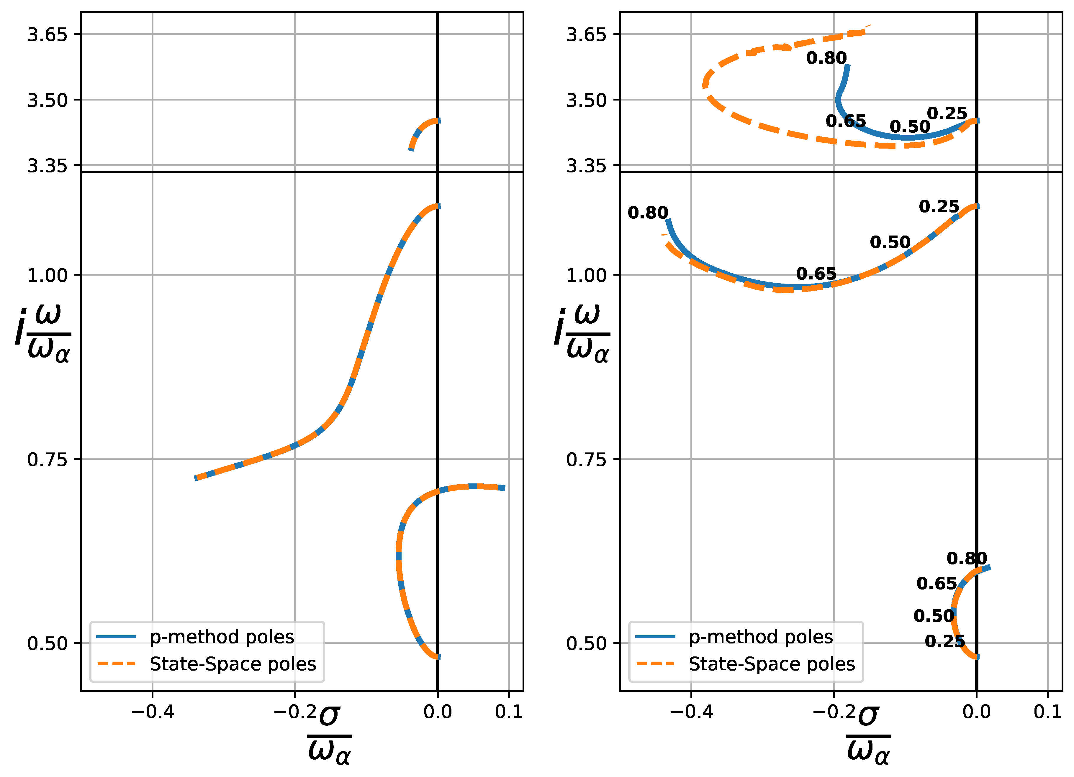
This time-invariant system is validated by comparing the root locus of a typical airfoil obtained using the p-method with the poles of the state-space model and the RFA applied, as illustrated in Figure 2. The specific airfoil parameters are detailed in Table 1, extracted from Edward’s work[13]. This system will be used to present the results obtained throughout the paper.

In this context,

x_{α}

represents the nondimensional distance from the center of mass to the elastic axis,

r_{α}^{2}

the nondimensional radius of gyration of the airfoil,

x_{δ}

the nondimensional distance from the center of mass of the control surface to the hinge axis, and

r_{δ}^{2}

stands for the nondimensional radius of gyration of the control surface. Additionally, a corresponds to the nondimensional location of the elastic axis, c to the nondimensional separation between the elastic axis and the hinge axis of the control surface, and

ζ_{δ}

denotes the nondimensional damping coefficient of the control surface mode.

It is seen that while for the incompressible regime our state-space analysis closely matches the results derived from the exact Theodorsen solution [16] expressed in the Laplace plane [12,13]. However, in the case of compressible flow, we notice a significant mismatch in the aileron mode. This difference can be attributed to inaccuracies in our fitting process, where the frequency is either too high or far from the imaginary axis. Despite these discrepancies, we’ll proceed our calculations as the plunging and torsion modes align well with our model.

3. Standard compensator

In order to stabilize the system, the following approach involves the implementation of a control law based on the state-space system. Various control strategies have been studied either theoretically or implemented in active flutter suppression, including PID control, pole-placement, the Linear Quadratic Regulator (LQR) method, and Kalman filters[17], among other options. In this work, a first approach will be to study the stabilization of the system by the use of pole-placement and LQR method.

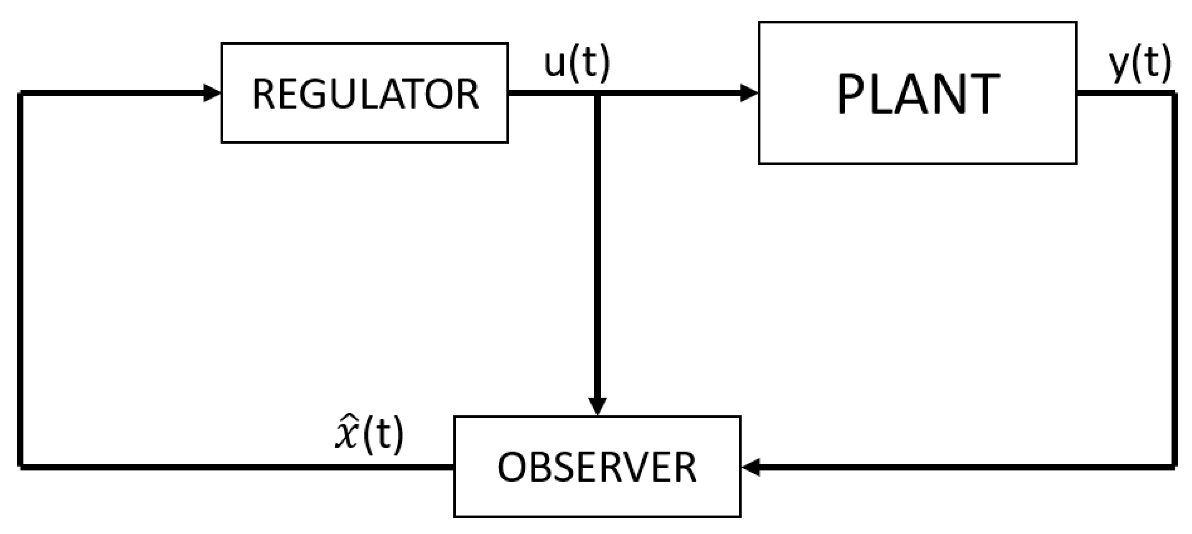
The control loop can be split into two essential parts, each serving a specific role in the overall control strategy. First, we have the feedback gain matrix, known as K, which is responsible for generating the control input u. This input relies on the estimated full state vector,

\hat{x}

, representing the internal states. These states are estimated using a linear observer, which uses the system’s output vector y to track the system evolution over time. The separation principle states that the regulator and the estimator can be implemented separately, simplifying the control system design. The implementation of an observer together with a regulator is often referred to as a compensator.

In this section, a control law will be derived based on the previously presented state-space system. First, the state-space system will be completed. Subsequently, an examination of the system’s controllability and observability will be undertaken. Then, an observer and a regulator will be separately obtained. Finally, the effectiveness and efficiency of the resulting control law will be assessed.

3.1. Completion of the state-space model

The state-space system presented in Equation 8 must be completed, since it only has information of the states of the system and its inputs. To accomplish this, the output matrix, C is defined here. In our particular system, the moment applied to the control surface cannot be measured directly, so the direct transmission matrix of the system, D, is set to zero. Hence, the output equation is:

y = C x + D u = C x

(10)

As established earlier, the system’s states include both physical and aerodynamic states. Only the physical states (h,

α

δ

and its derivatives) can be measured directly, therefore the output matrix is defined as:

C = [\begin{matrix} {[\begin{matrix} I \end{matrix}]}_{6 x 6} & {[\begin{matrix} 0 \end{matrix}]}_{6 x (N - 2))} \end{matrix}]

(11)

In this case, it is assumed that we are measuring all physical states of the system. In practice, one should include here only the states that can be measured using the available sensor infrastructure.

Gathering the state-space matrices, a linear time-invariant system is obtained, represented through the standard formulation:

\begin{matrix} \begin{matrix} s x & = A x + B u \\ y & = C x \end{matrix} \end{matrix}

(12)

3.2. Controllability matrix

Given the high number of states (

6 + 3 (N - 2)

) compared to the number of control inputs (1), it is possible that the system is not fully controllable. The controllability matrix[18] is defined as:

P = [\begin{matrix} B & A B & A^{2} B & . . . & A^{n - 1} B \end{matrix}]

(13)

with n being the rank of matrix A.

By definition, a system is considered controllable if the rank of its controllability matrix matches the rank of the system itself. As expected, the investigated airfoils are uncontrollable. Nevertheless, an uncontrollable system may still be stabilizable. This can be achieved by breaking down the system into controllable and uncontrollable subsystems and, providing that the uncontrollable one is stable, a control law can be derived that stabilized the full system. The decomposition will be carried out hereafter.

3.3. Decomposition into controllable and uncontrollable subsystems

Let P be the controllability matrix of the system, and assume

rank (P) \equiv q < n

. An invertible matrix

T \in R^{n x n}

can be found that transform the system into its echelon form:

T P \equiv \tilde{P} = [\begin{matrix} \tilde{P_{1}} \\ 0 \end{matrix}]

(14)

Let

\tilde{x} = T x = {[\begin{matrix} {\tilde{x}}_{c} & {\tilde{x}}_{u} \end{matrix}]}^{T}

be the new states, with

{\tilde{x}}_{c}

and

{\tilde{x}}_{u}

being the controllable and uncontrollable states. The state-space system then becomes:

\begin{matrix} \begin{matrix} s \tilde{x} & = T A T^{- 1} \tilde{x} + T B u = \tilde{A} \tilde{x} + \tilde{B} u \\ y & = C T^{- 1} \tilde{x} = \tilde{C} \tilde{x} \end{matrix} \end{matrix}

(15)

The resulting matrices

\tilde{A}

\tilde{B}

have the form

\tilde{A} = [\begin{matrix} A_{c} & A_{12} \\ 0 & A_{u} \end{matrix}], \tilde{B} = [\begin{matrix} B_{c} \\ 0 \end{matrix}]

(16)

The system

A_{c}

can be controlled independently from

A_{u}

, since

eig (A) = eig (A_{c}) \cup eig (A_{u})

(17)

Now, a control law can be developed that feeds the controllable states to the input, following the expression

u = K_{c} {\tilde{x}}_{c}

. The control matrix

K_{c}

can be obtained for the subsystem (

A_{c}

B_{c}

) via pole-placement or any other method. To apply the resulting matrix to the original system, the similarity transformation is reversed:

u = K x = \tilde{K} T x = [\begin{matrix} K_{c} & 0 \end{matrix}] T x

(18)

3.4. Regulator implementation

In order to achieve the desired behaviour of the system, the pole-placement method is introduced. This technique is based on the canonical transformation of the system, with its algorithm for MIMO systems presented by Nguyen [19,20].

The application of this algorithm yields a feedback matrix tailored to the controllable subsystem. Following Equation 18, the resulting control law takes the full state as an input:

u = K x

(19)

However, conventional pole-placement arises numerical instabilities during the algorithm implementation. While such instabilities may not significantly impact systems with a limited number of states, due to the large number of aerodynamic states created in this model, an exact placement of the poles cannot be achieved. Valášek and Olgac[21] present a modified approach that minimizes these errors.

The primary challenge in this method lies in the arbitrary selection of the target poles, which often overlooks the significance of the controller’s own poles. The ramifications of this choice will be exposed later.

3.5. Linear observer implementation

A linear observer, often referred to as a state observer or estimator, mimics the behaviour of the system, using available sensor measurements and knowledge of the system’s dynamics. Since the model is a representation of reality, it will not be exact, due to nonlinearities in the original model or to modelling inaccuracies. To amend these differences, the observer is corrected with the available system output. The state equation governing the observer’s behavior is as follows:

\begin{matrix} \begin{matrix} s \hat{x} & = A \hat{x} + B u + L (y - \hat{y}) \\ \hat{y} & = C \hat{x} \end{matrix} \end{matrix}

(20)

with L being the observer gain matrix.

Since the estimated output is available from the second equation, the system can be expressed as:

s \hat{x} = (A - L C) \hat{x} + B u + L y

(21)

The observer’s dynamics is given by the eigenvalues of the matrix

A - L C

. The observer matrix can then be obtained by pole-placement or other methods in a similar manner to the regulator gain, replacing A and B with

A^{T}

and

C^{T}

. It is essential that the observer’s poles are positioned significantly distant from those of the regulator, so the dynamics of the estimated states be faster than those of the regulator. A common practice involves placing the observer poles 10 times farther than those of the regulator.

In this particular case, the matrix L will be computed by the use of a Linear Quadratic Regulator (LQR). The primary objective of LQR is to determine the adequate control inputs that minimize a quadratic cost function. This cost function typically includes terms related to the state of the system and the control input. Consequently, the primary challenge is to find an equilibrium between control effort and performance trade-offs.

3.6. Closed-loop dynamics

After determining the observer gain matrix L and the regulator matrix K, the dynamics of the state-space model is presented and a control law that ensures system stability will be derived.

Mapping the regulator inputs to the estimated state,

u = K \hat{x}

and incorporating the feedback gain into Equation 21 leads us to the following equation:

s \hat{x} = (A + B K - L C) \hat{x} + L y

(22)

where

y = C x

represents information obtained from the original plant. Combining the observer dynamics with the primary state-space model, we obtain an extended representation of the state-space model governing the closed-loop system, expressed as:

\{\begin{matrix} s x \\ s \hat{x} \end{matrix}\} = [\begin{matrix} A & B K \\ L C & A + B K - L C \end{matrix}] \{\begin{matrix} x \\ \hat{x} \end{matrix}\}

(23)

This extended system allows us to derive the controller. Based on Equation 22, the control law is presented as a transfer function like:

u = K {(s I - A + B K - L C)}^{- 1} L y = K_{C o m p} y

(24)

This is the final control law, that stabilizes the state-space model. It relies only on measurable outputs, as well as the system’s reduced frequency. Its analysis in the Laplace domain and its practical implementation for an airfoil system can be carried out following the schematic block-diagram depicted in Figure 3.

3.7. Specific control law and results

To proceed with the actual implementation of the control law, the parameters for the pole-placement and the LQR observer must be configured. To ensure adequate system stability, a stability margin is defined to prevent the poles from approaching the imaginary axis too closely. The stable poles in the closed loop are positioned at the same locations as the open-loop branches, while those on the unstable branches are adjusted to maintain the specified stability margin. For the weight and cost matrices of the LQR controller, identity matrices are selected. For improved performance, the results can be tuned with these matrices.

To circumvent potential inaccuracies arising from the aerodynamic model approximation, the p-method is employed to compute the pole locations. The control law has been computed based on the extended system, as illustrated in Equation 23. However, to make it applicable to the original model, it must be integrated into Equation 2. Considering that the control law relies on the original states

x_{q}

and their derivatives, the following matrix is included in the feedback gain:

y = [\begin{matrix} I \\ s I \end{matrix}] x_{q}

(25)

Consequently, the dynamic equation for the system incorporating the control law takes the form:

[M_{s} {(\frac{U}{b})}^{2} s^{2} + B_{s} (\frac{U}{b}) s + K_{s} - \frac{η}{2} {(\frac{U}{b})}^{2} Q (s) - G K_{C o m p} (s) [\begin{matrix} I \\ s I \end{matrix}]] x_{q} = 0

(26)

with the feedback matrix defined as:

K_{C o m p} (s) = K {(s I - A + B K - L C)}^{- 1} L

(27)

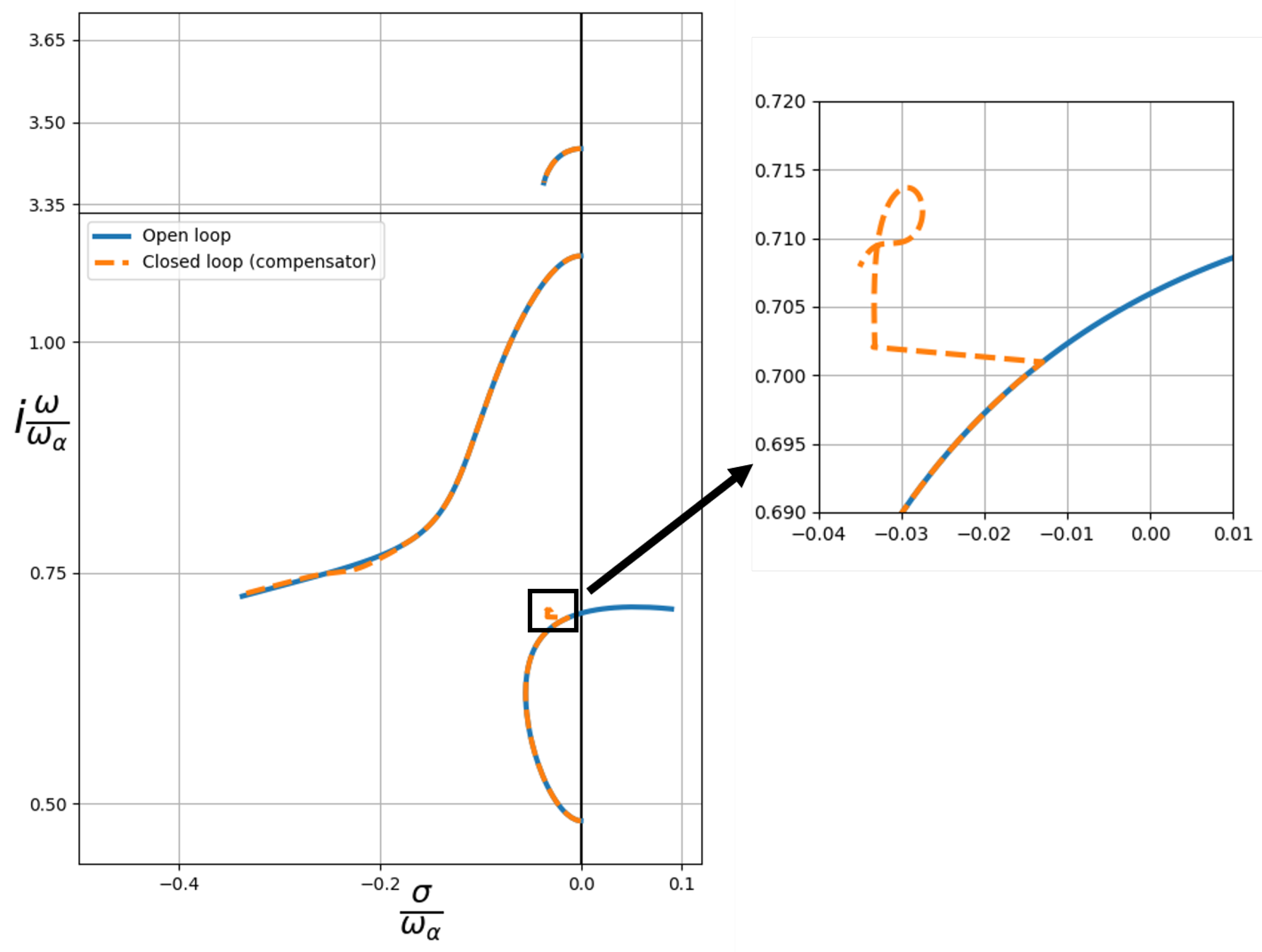
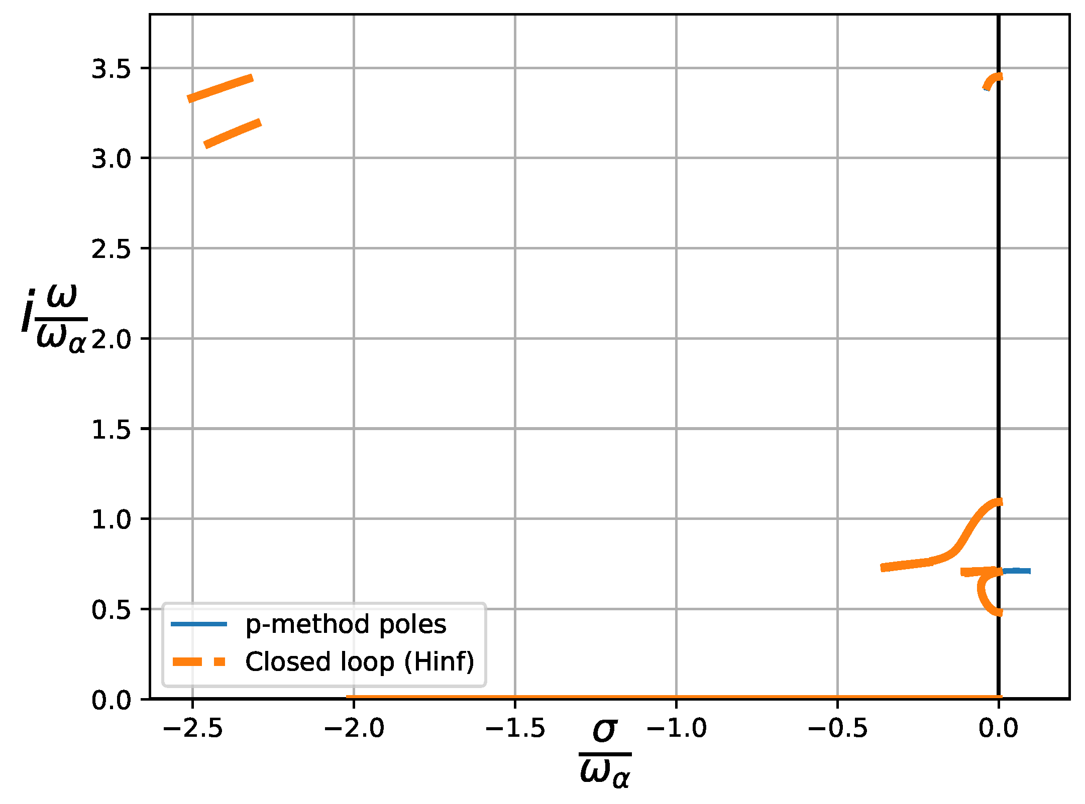
We initiate the analysis by plotting the root locus of the closed-loop system for the airfoil parameters listed in Table 1, as depicted in Figure 4. The control law is activated when an open-loop pole approaches the stability margin, effectively maintaining system stability for every airspeed. The originally unstable branch remains in the left plane, maintaining an stability margin from the imaginary axis. Furthermore, the system’s branches remain continuous, ensuring the smooth operation of the control law across all velocities.

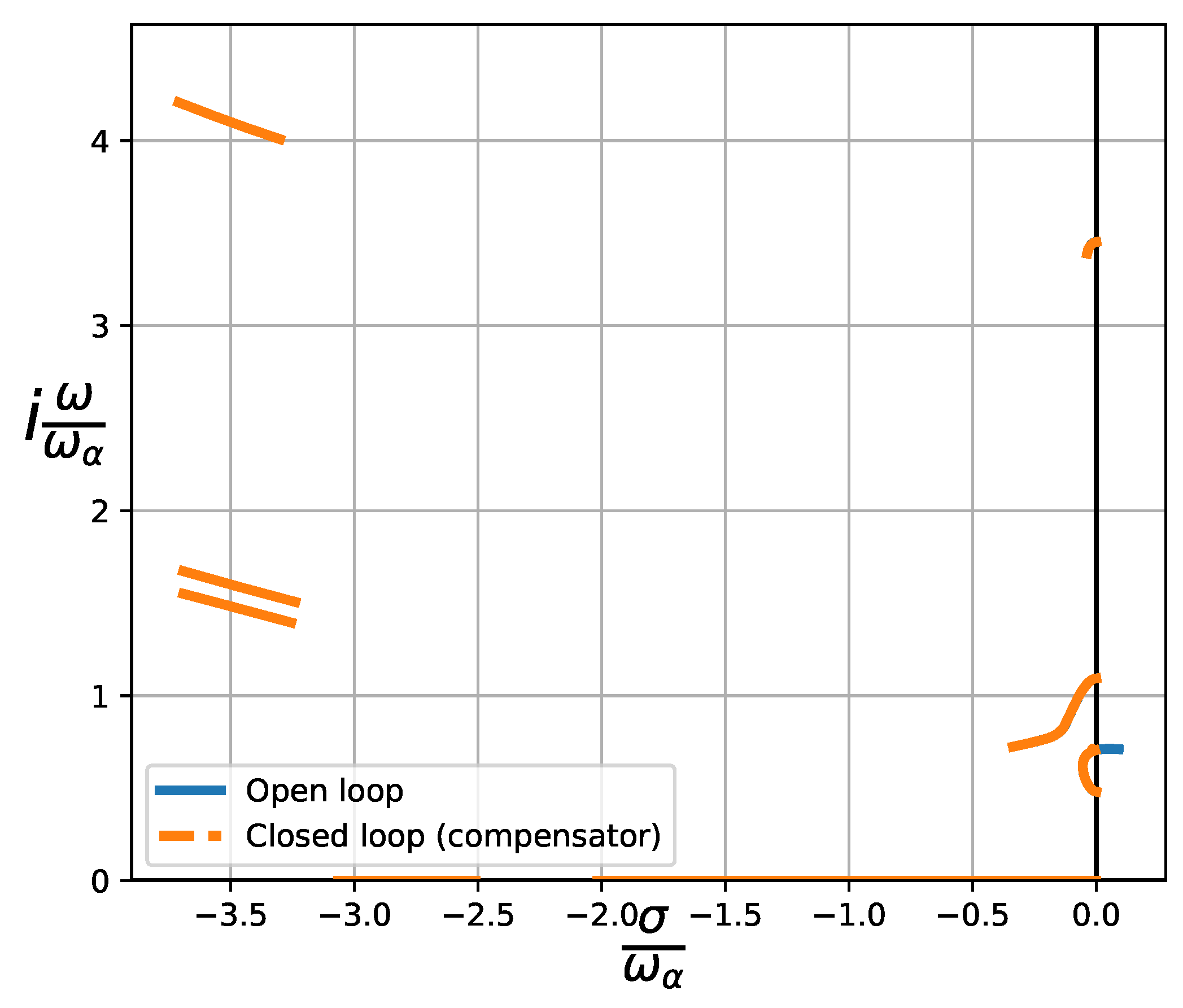
Figure 5 shows the same results, focusing on the rest of the poles from the state-space system. As anticipated, new branches emerge in the left plane, relating to the compensator poles, whose characteristics are directly influenced by the chosen control law parameters. This inherent dependence on parameter selection highlights a key limitation of this approach, as the resulting system dynamics are arbitrarily shaped by these choices.

4. $H_{\infty}$ controller

In the preceding section, the controller derived exhibited a degree of arbitrariness due to the influence of the chosen weighting matrices within the Linear Quadratic Regulator (LQR) framework, as well as the arbitrary location of the poles. This section aims to procure an optimal controller to overcome these issues.

For this purpose, it is imperative to establish a clear definition of optimality. The primary objective herein is to formulate a controller that accomplishes system stabilization while minimizing the energy consumption. Additionally, the optimal controller should demonstrate efficiency across a broad spectrum of frequencies, obviating the need for frequency-specific tuning. With these objectives in mind, the

H_{\infty}

norm of a system is introduced here.

The

H_{\infty}

(H-infinity) norm is a fundamental concept in control theory and signal processing. It serves as a critical measure of the frequency-domain performance of a system, offering insights into its robustness and stability characteristics. The H-infinity norm quantifies the maximum gain from a given input to the system’s output across all frequencies, making it a powerful tool for assessing a system’s susceptibility to external disturbances and uncertainties. In essence, it provides a means to evaluate the worst-case behavior of a system, which is essential for designing robust control systems and ensuring that they perform reliably under a variety of real-world conditions. Moreover,

H_{\infty}

control does not require a precise model of the system. It can accommodate modeling errors and uncertainties, making it suitable for real-world systems where accurate modeling can be challenging.

In the upcoming section, we commence by exploring the computation of the

H_{\infty}

norm. We then shift our focus to the aggregate plant, where we consider a multidimensional system encompassing various inputs and outputs, emphasizing the minimization of the

H_{\infty}

norm for regulated outputs. Next, we investigate suboptimal

H_{\infty}

controller design, highlighting an iterative approach and the advantages of closed-form solutions. Finally, we address the issue of strong stabilization, ensuring controller stability in the presence of various factors, and present a methodology for achieving internal stability. Together, these sections provide a comprehensive overview of the application

H_{\infty}

control to flutter alleviation systems, emphasizing the pursuit of optimal system performance while maintaining stability and reliability.

4.1. Computation of the $H_{\infty}$ norm

As it has been stated, the

H_{\infty}

norm measures the worst-case behaviour of a system. This assessment is achieved through the computation of the maximum singular value, denoted as

σ_{max}

, across the entire frequency domain for a given transfer function,

G (j ω)

. Consequently, the

H_{\infty}

norm is formally expressed as:

{|| G ||}_{\infty} : = sup_{ω} σ_{max} [G (j ω)]

(28)

Traditionally, this computation would include a Bode plot, in which the maximum response of the system would be obtained. However, Boyd, Balakrishnan, and Kabamba [9] introduced an algorithmic approach for the expedient numerical estimation of the

H_{\infty}

norm. The fundamental steps of this algorithm are as follows:

Select an initial guess for value for the norm of the system, $γ$ .
Define the Hamiltonian matrix

$H : = [\begin{matrix} A - B R^{- 1} D^{T} C & - γ B R^{- 1} B^{T} \\ γ C^{T} S^{- 1} C & - A^{T} + C^{T} D R^{- 1} B^{T} \end{matrix}]$

(29)

where $R = (D^{T} D - γ^{2} I)$ and $S = (D D^{T} - γ^{2} I)$ .
Check if H has no eigenvalues on the imaginary axis. If so, then ${|| G ||}_{\infty} < γ$ , and $γ$ is subsequently decreased. Else, increase $γ$ .
Repeat. The calculations finish when the solution converge to ${|| G ||}_{\infty} = γ$ .

This method enables a more systematic and mathematically rigorous approach, reducing the reliance on graphical techniques and facilitating the optimization of systems that demand stringent performance criteria.

4.2. Aggregate plant

The

H_{\infty}

control method considers not only the closed-loop system’s stability but also aims to minimize the control effort and estimation errors. Hence, the system input and outputs must be expanded to account for these variables.

For this purpose, the system is represented as a 9-matrices system, resulting in the creation of an aggregate plant with an augmented set of inputs and outputs. As depicted in Figure 6, the expanded plant includes the following categorizations for inputs and outputs:

Exogenous inputs w: unmodelled dynamics, sensor noise, tracking signal.
Actuator inputs u: effect of actuators.
Regulated outputs z: states to be minimized.
Sensed outputs y: states that can be measured.

The dynamic equations governing the relationships among these variables are expressed

\begin{matrix} \begin{matrix} s x & = A x + B_{1} w + B_{2} u \\ z & = C_{1} x + D_{11} w + D_{12} u \\ y & = C_{2} x + D_{21} w + D_{22} u \end{matrix} \end{matrix}

(30)

Since the objective is to minimize the effect of the exogenous inputs on the regulated outputs, the exogenous inputs must include not only potential noise and inaccuracies but also account for actuator inputs. In the context of our airfoil system, the aggregate plant, when realized in its 9-matrices representation, takes the form:

[\begin{array}{c} A & B_{1} & B_{2} \\ C_{1} & D_{11} & D_{12} \\ C_{2} & D_{21} & D_{22} \end{array}] = [\begin{array}{c} A & [\begin{matrix} B & 0 \end{matrix}] & B \\ [\begin{matrix} C \\ 0 \end{matrix}] & 0 & [\begin{matrix} 0 \\ I \end{matrix}] \\ C & [\begin{matrix} 0 & I \end{matrix}] & 0 \end{array}]

(31)

The stabilization of the aggregate plant is achieved through the incorporation of a feedback loop from the sensed outputs to the actuator inputs. In the closed-loop configuration, the primary objective of this section is to minimize the H-infinity norm of the transfer function from exogenous inputs to regulated outputs, denoted as

{|| T_{z w} ||}_{\infty}

4.3. Suboptimal $H_{\infty}$ controller

Various methodologies for computing an H-infinity controller are available within the control theory domain. Notably, Gahinet and Apkarian[11] presented a method for obtaining an optimal H-infinity controller with the introduction of Linear Matrix Inequalities (LMIs). This optimization framework relies on Semi-Definite Programming (SDP) and is solved through the utilization of convex optimization and Interior-Point optimization algorithms[22][23]. Nevertheless, the original method lacks the flexibility to incorporate specific constraints or limitations. Addressing this limitation, Chilali and Gahinet[10] included the use of Pole Placement Constraints, which can be employed, for instance, to restrict the velocity of the resultant controller. Furthermore, Scherer, Gahinet, and Chilali[24] expanded the method by enabling the incorporation of multi-objective output-feedback optimization.

However, the direct optimization approach using LMIs is considered less suitable for its use in this work. Firstly, the resulting controller is not guaranteed to possess internal stability, which is a crucial attribute for controller performance. Secondly, the computation of suboptimal H-infinity controllers presents a closed-form solution, which renders it a more time-efficient strategy. Consequently, in this case it is more advantageous to derive first suboptimal H-infinity controllers and subsequently search for the optimal controller.

The objective of suboptimal

H_{\infty}

controllers will be to find all admissible controllers K such that

{T_{z w}}_{\infty} < γ

, given an arbitrary scalar

γ

. Doyle el al.[25] present a method to compute this controller, based on the solution to two Algebraic Riccati Equations (ARE). The algorithm is presented hereafter.

For a given

γ

, define the following Hamiltonian matrices:

H_{\infty} = [\begin{matrix} A & γ^{- 2} B_{1} B_{2}^{T} - B_{2} B_{2}^{T} \\ - C_{1}^{T} C_{1} & - A^{T} \end{matrix}], J_{\infty} = [\begin{matrix} A^{T} & γ^{- 2} C_{1}^{T} C_{1} - C_{2}^{T} C_{2} \\ - B_{1} B_{1}^{T} & - A \end{matrix}]

(32)

An admissible controller such that

{T_{z w}}_{\infty} < γ

exists if and only if the following conditions hold:

$H_{\infty} \in dom (Ric)$ and $X_{\infty} : = Ric (H_{\infty}) \geq 0$
$J_{\infty} \in dom (Ric)$ and $Y_{\infty} : = Ric (J_{\infty}) \geq 0$
$ρ (X_{\infty} Y_{\infty}) < γ^{2}$

with

Ric (H_{\infty})

being the Riccati operator,

ρ

the spectral radius, and with

Ric (H_{\infty}) \geq 0

being an LMI, i.e., it refers to the real part of the eigenvalues of

Ric (H_{\infty})

If the three conditions above are fulfilled, then the suboptimal controller is defined as:

K_{s u b} : = [\begin{array}{c} {\hat{A}}_{\infty} & - Z_{\infty} L_{\infty} \\ F_{\infty} & 0 \end{array}]

(33)

where

\begin{matrix} {\hat{A}}_{\infty} : = A + γ^{- 2} B_{1} B_{1}^{T} X_{\infty} + B_{2} F_{\infty} + Z_{\infty} L_{\infty} C_{2} \\ F_{\infty} : = - B_{2}^{T} X_{\infty} \\ L \infty : = - Y_{\infty} C_{2}^{T} \\ Z_{\infty} : = {(I - γ^{- 2} Y_{\infty} X_{\infty})}^{- 1} \end{matrix}

In order to find an optimal controller, an iterative procedure in

γ

is implemented, searching for its minimum value. The implementation of this control strategy demonstrates efficient computation, since the solution to Riccati equations is constructed directly from the eigenvectors of both the

H_{\infty}

and

J_{\infty}

matrices. However, it must be noted that the proof of this algorithm does not ensure the internal stability of the controller. Remarkably, in the cases studied in this paper, the controller obtained is internally unstable, i.e. some poles of the controller are in the right half-plane. The stabilization of the controller is regarded below.

4.4. Strong stabilization

As it has been stated, one notable concern with the

H_{\infty}

approach is the fact that internal stability is not guaranteed[26]. The concept of internal stability remains crucial when implementing such controllers, as any deviation could lead to numerical errors and erratic controller behavior. Consequently, assuring the stability of an

H_{\infty}

design is imperative and demands independent verification.

The foundation of this control strategy rests on the distinct and unique stabilizing solution to the Riccati equations, resulting in what is commonly referred to as the "central controller". Nevertheless, a family of admissible controllers that fulfil the condition

{T_{z w}}_{\infty} < γ

exists. Doyle[25] obtains them through the application of a linear-fractional transformation (LFT[27]) between the central controller and an arbitrary matrix

A_{q}

. The central controller has the following form:

K_{\infty} (s) = [\begin{array}{c} A_{c} & B_{c 1} & B_{c 2} \\ C_{c 1} & D_{c 11} & D_{c 12} \\ C_{c 2} & D_{c 21} & D_{c 22} \end{array}] = [\begin{array}{c} {\hat{A}}_{\infty} & - Z_{\infty} L_{\infty} & Z_{\infty} B_{2} \\ F_{\infty} & 0 & I \\ - C_{2} & I & 0 \end{array}], {|| Q ||}_{\infty} < γ

(34)

Based on this family of controllers, several authors have dealt with this problem. Campos-Delgado and Zhou[28] adopt an iterative approach to stabilize the original controller, creating a series of nested feedback loops. In this case, the main problem lies in the order of the resulting controller, since with each control loop the order increases linearly. Most authors propose a solution based on coprime factorization[29,30].

Here, the approach proposed by Zeren and Özbay[31], which is built around the solution to two additional Algebraic Riccati Equations (AREs) will be applied.

For the existence of a stabilizing controller, the following conditions are necessary:

$(A_{c}, B_{c 2})$ is stabilizable and $(C_{c 2}, A_{c})$ is detectable
$A_{c}$ has no eigenvalues in the imaginary axis

Provided these conditions are fulfilled, then the stabilizing solution X to the following ARE is computed:

A_{c}^{T} X + X A_{c} - X B_{c 2} B_{c 2}^{T} X = 0, X = X^{T} \geq 0

(35)

Then, an stabilizing controller exists if a stabilizing solution exists for the ARE:

A_{X} Y + Y A_{X}^{T} - Y (ρ^{2} C_{c 2}^{T} C_{c 2} - X B_{c 2} B_{c 2}^{T} X) Y + B_{c 2} B_{c 2}^{T} = 0, Y = Y^{T} \geq 0

(36)

with

ρ

being an arbitrary scalar and

A_{X} = A - B_{c 2} B_{c 2}^{T} X, F = - B_{c 2}^{T} X

Under this sufficient condition,

K_{q} (s) = [\begin{array}{c} A_{q} & B_{q} \\ C_{q} & D_{q} \end{array}] = [\begin{array}{c} A_{K} & - L \\ F & 0 \end{array}]

(37)

is a strongly stabilizing controller with

K_{\infty} \leq ρ

, where

A_{K} = A_{c} + B_{c 2} F + L C_{c 2}, L = - ρ^{2} Y C_{c 2}^{T}

Since Equation 34 stated that the subcontroller must have

H_{\infty}

norm under

γ

, then the calculation of the subcontroller

K_{q}

is an iterative procedure, starting with

ρ = γ

, with

ρ

being subsequently decreased so as to find an optimal subcontroller. In case that for

ρ = γ

a solution to the aforementioned AREs cannot be reached, then there does not exist an stabilizing controller.

With this additional feedback loop, the final state-space system of the controller corresponds to the linear fractional transformation

K (s) = LFT (K_{\infty}, K_{q})

. Its state-space form is depicted as follows:

K (s) = [\begin{array}{c} A_{K \infty} & B_{K \infty} \\ C_{K \infty} & 0 \end{array}] = [\begin{array}{c} [\begin{matrix} A_{c} & B_{c 2} C_{q} \\ B_{q} C_{c 2} & A_{q} \end{matrix}] & [\begin{matrix} B_{c 1} \\ B_{q} D_{c 21} \end{matrix}] \\ [\begin{matrix} C_{c 1} & D_{c 12} C_{q} \end{matrix}] & 0 \end{array}]

(38)

Following the same procedure as in the case of the compensator, the controller system is expressed in its transfer function form. This is required so as to be able to apply the p-method in the Laplace plane. The control law is then:

u = C_{K \infty} {(s I - A_{K \infty})}^{- 1} B_{K \infty} y

(39)

Equations 25 and 26 are then used to obtain the dynamic equation of the system in closed loop, substituting the compensator control law by the one here presented.

4.5. Specific control law and results

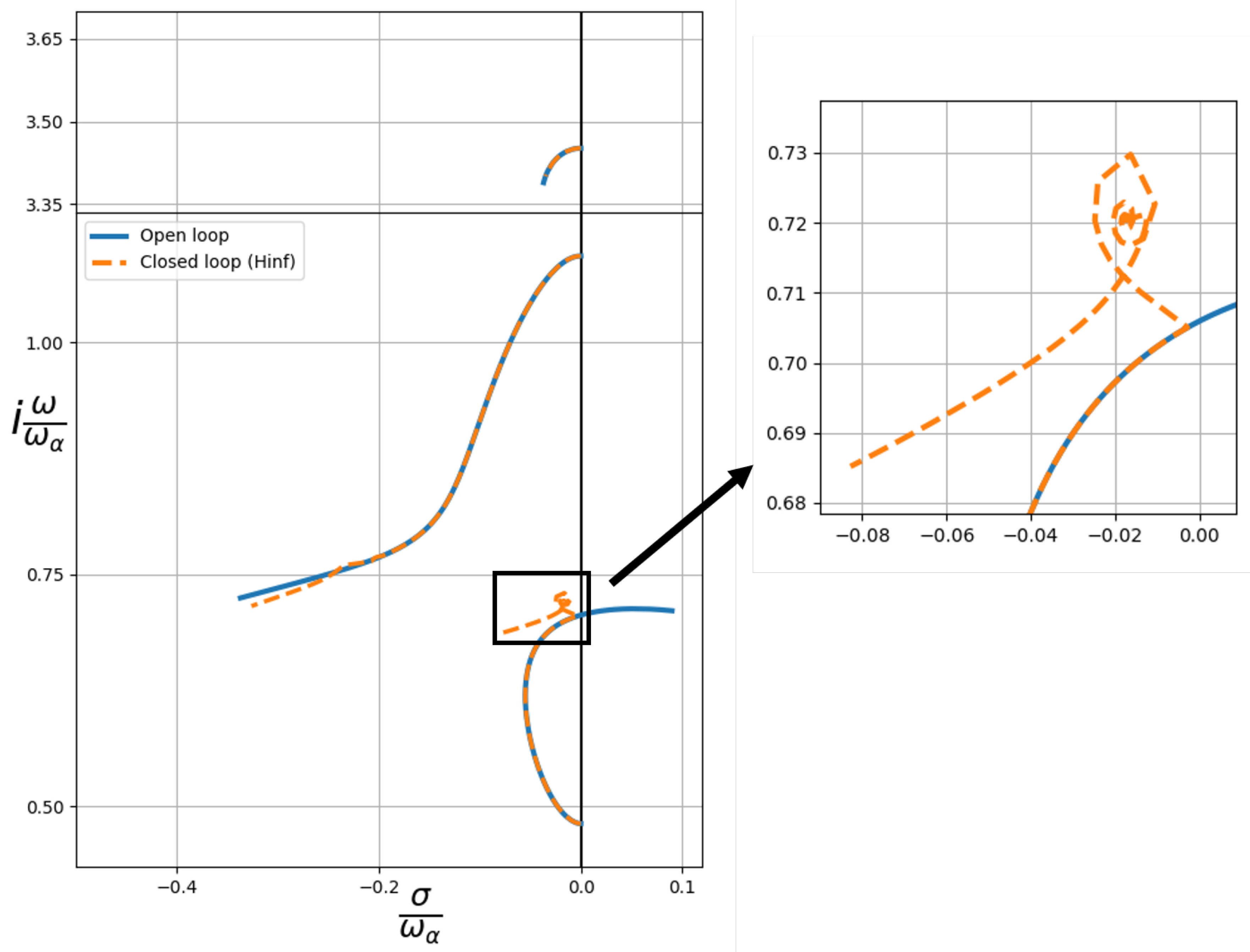
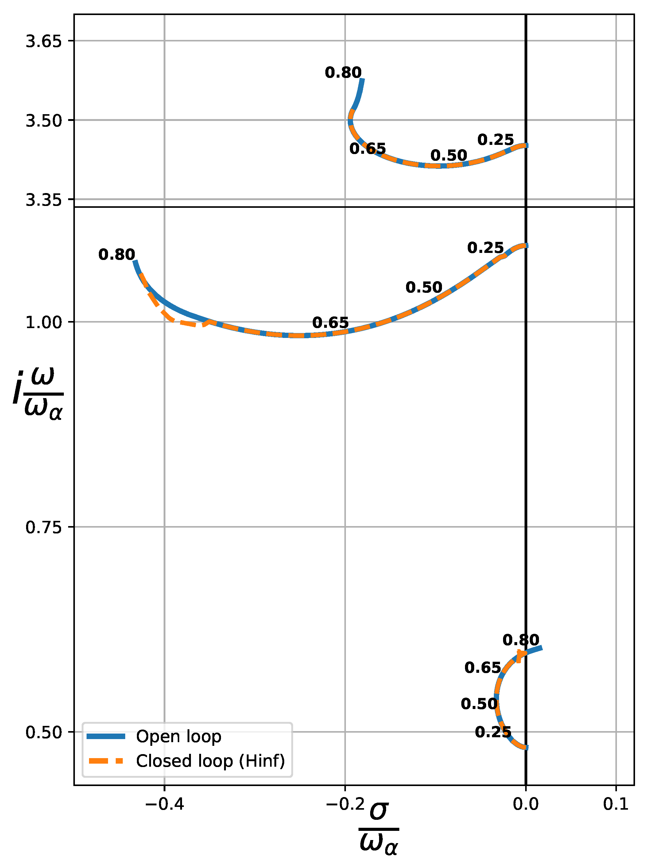
Once again, the control procedure is tested on the airfoil in incompressible regime. Figure 7 shows the results. It can be seen that the branch corresponding to the plunging mode is stabilized before approaching the imaginary axis, averting any potential flutter issues. It is interesting to mention that after mitigating flutter, the system not only remains stable but also moves away from the imaginary axis.

In Figure 8, we present the system’s pole distribution across the complete Laplace plane. A set of new branches has emerged, positioned significantly distant from the imaginary axis, as in the previous case. Unlike the compensator scenario, the closed-loop poles in this case proves to be optimal, and does not depend on arbitrary parameters.

5. Results for a three dof airfoil

Following the results presented above for the closed loop dynamics of the airfoil given in Table 1, a comparison of the two methods employed to obtain the control law is presented here. The effectiveness and efficiency of the system hinge upon the assessment of the

H_{\infty}

norm of the transfer function, specifically from exogenous inputs to regulated outputs, denoted as

{|| T_{z w} ||}_{\infty}

. It is essential to underscore that these regulated outputs encompass not only the system’s states but also its inputs. Hence, a higher norm implies higher control effort from the actuator, which, in turn, may cause mechanical wear and tear on the system’s actuators. Figure 9 shows this comparison. The

H_{\infty}

norm of the system in the case of the compensator is nearly two orders of magnitude higher than that of the

H_{\infty}

controller, thereby showing the efficiency of the

H_{\infty}

approach.

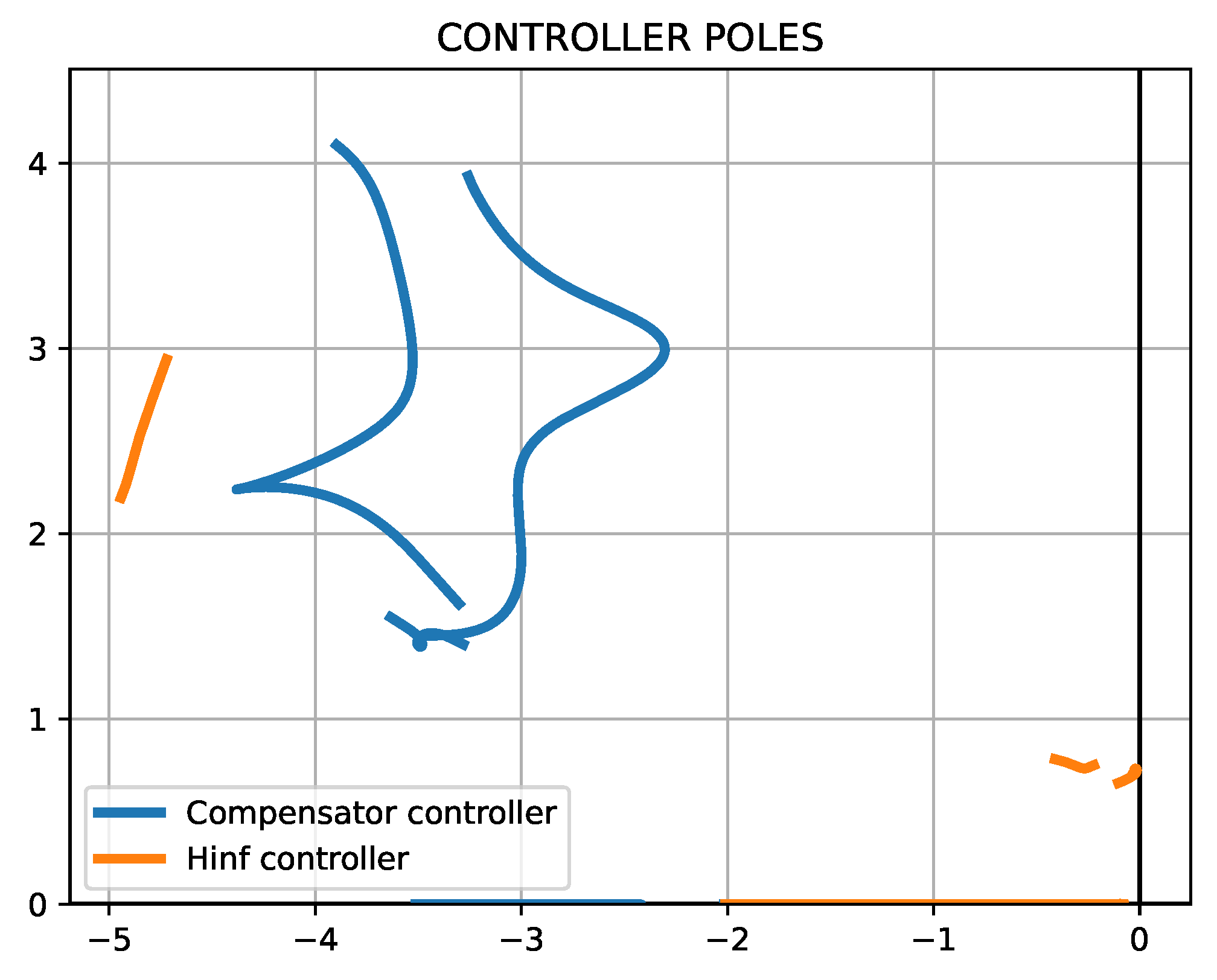
With respect to the dynamics of the control law, Figure 10 shows the root-locus of the two controllers. In both cases the resulting controllers are stable, a prerequisite for the practicable deployment of the control loop, as previously highlighted. However, it is pertinent to acknowledge that the natural frequencies of the

H_{\infty}

poles are lower than the ones from the compensator. This implies that the

H_{\infty}

controller does not require internal dynamics as fast as the compensator, which is a positive point for its implementation (faster controllers are usually more expensive, due to the necessity for high-speed processors and precision components to achieve rapid control responses).

Once the viability of this

H_{\infty}

implementation has been shown, it will be applied to a system in compressible regime. It is important to highlight the fact that even though the control law has been obtained using a state-space modelization of the system, it is applied to the exact dynamic equations, and computed via the p-method. This ensures that the results will be as close to reality as possible.

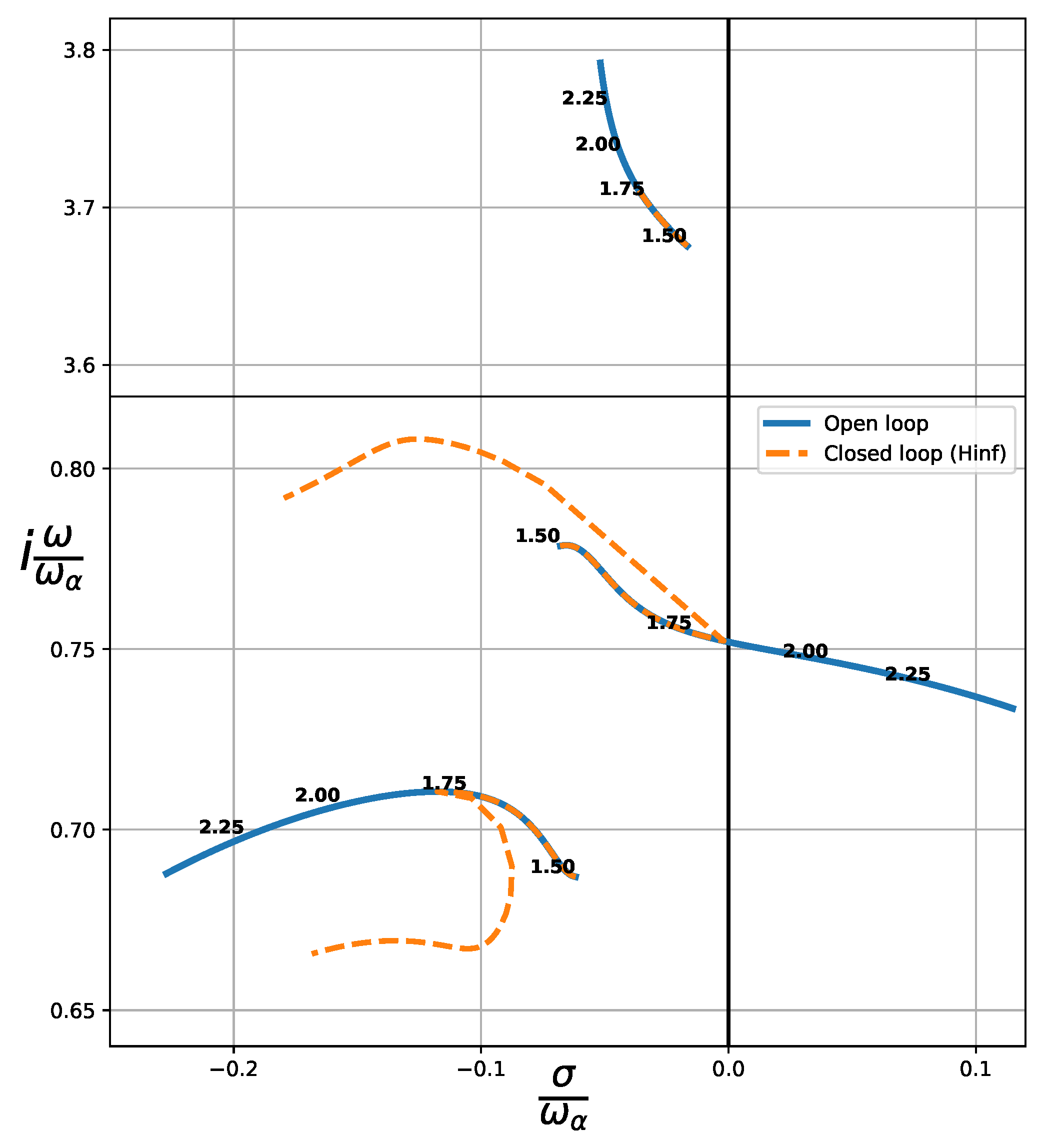
Figure 11 shows the root-locus for the aforementioned airfoil, operating within the subsonic regime, specifically up to Mach

0.8

. Similar to the incompressible case, the controller is able to stabilize the system without any problem. In this case, we observe the influence of the controller on the torsion branch, even though it has little effect on its stability.

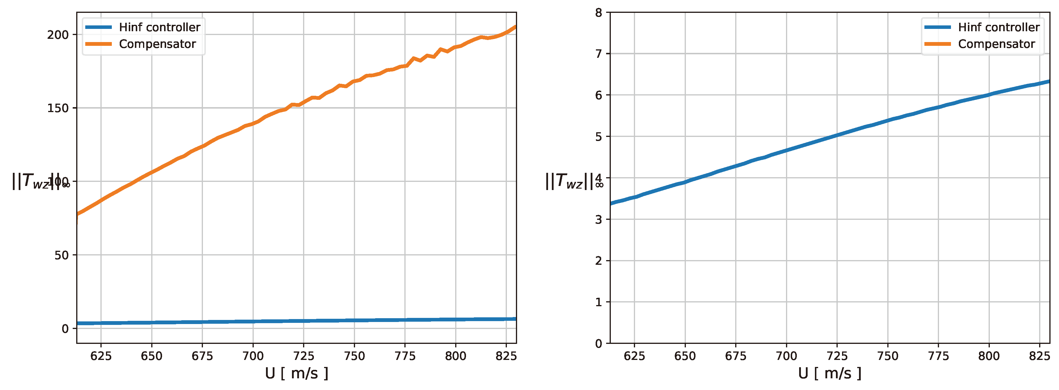
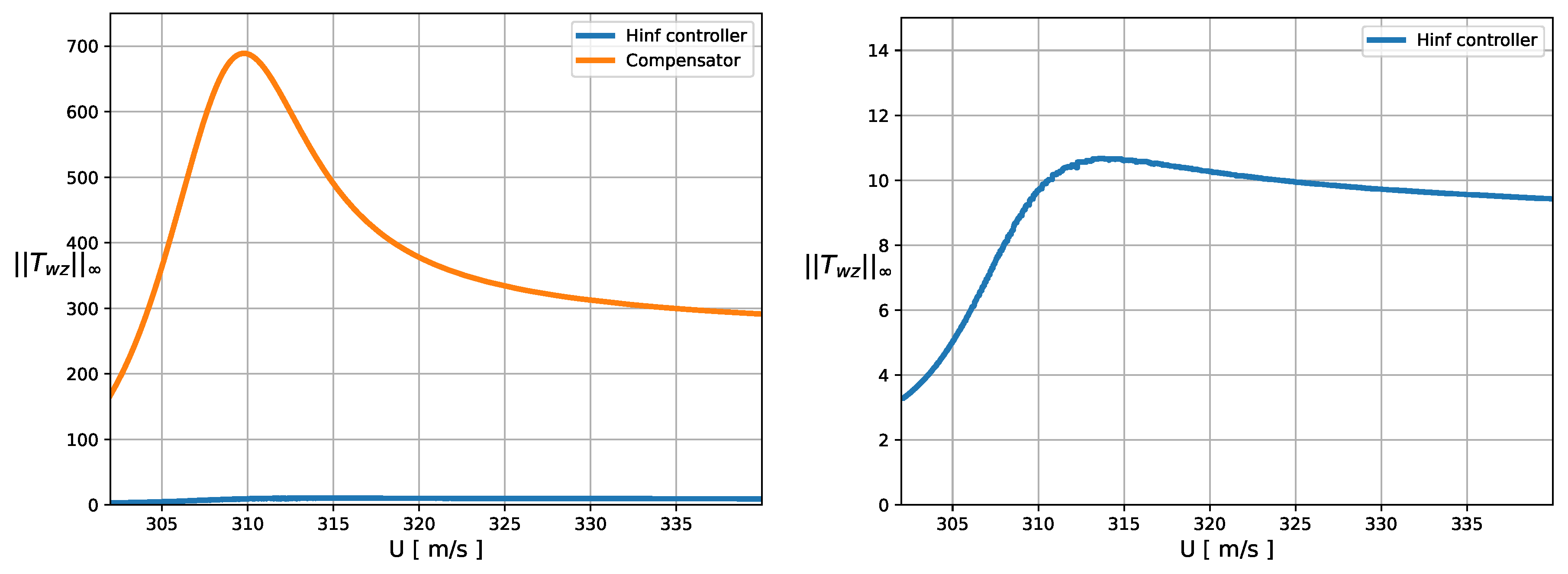
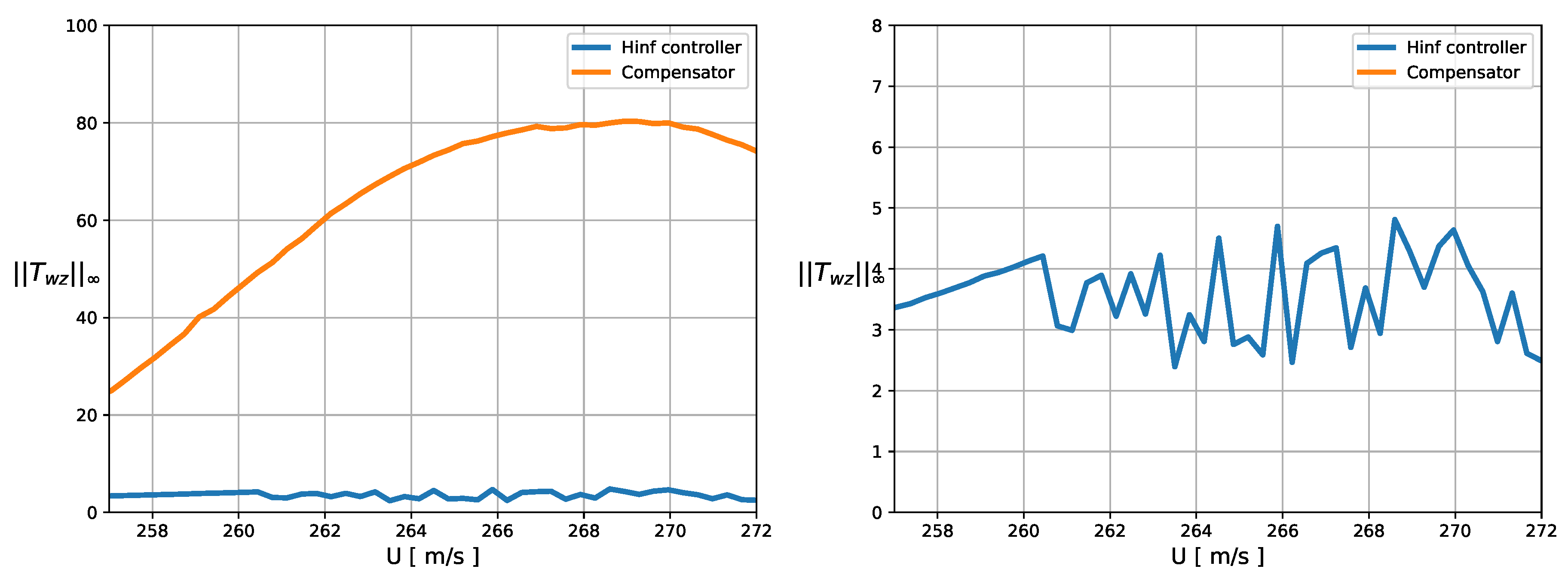
In the examination of the

H_{\infty}

norm for this closed-loop system, a noticeable dispersion in the results becomes apparent. This dispersion stems from the process of computing the state-space model for the airfoil, which involves determining the lags in Roger’s RFA through an optimization procedure. These lags are inherently dependent on the Mach number. While the approximate model closely mimics the exact one, it is essential to acknowledge that numerical optimization is executed for each specific Mach number. Consequently, the obtained lags exhibit non-smooth variations. One potential avenue to address this issue would involve the development of a regression model for the lags to ensure a smoother transition, though this solution requires further investigation to comprehensively consider all contributing factors.

Next, to assess the method’s suitability in supersonic regime, we introduce a different airfoil configuration, characterized by the parameters delineated in Table 2. A sweep in Mach number up to

M_{\infty} = 2.5

is performed, with

a_{\infty} = 333 m / s

. The behaviour of both the plunging and torsion modes is modified. Initially, the lower branch approaches the imaginary axis, subsequently reversing its direction. As the Mach number increases, all the modes seem to increase their stability. Regarding its performance, the

H_{\infty}

controller performance also exceeds that of the compensator in this regime.

Figure 13. Root-locus of a 3 dof airfoil in supersonic regime with a

H_{\infty}

controller. Mach numbers up to

2.5

are considered.

Figure 13. Root-locus of a 3 dof airfoil in supersonic regime with a

H_{\infty}

controller. Mach numbers up to

2.5

are considered.

Figure 14. Evaluation of the

{T_{z w}}_{\infty}

norm a the closed loop system in supersonic regime, comparing compensator and

H_{\infty}

controller efficiency.

Figure 14. Evaluation of the

{T_{z w}}_{\infty}

norm a the closed loop system in supersonic regime, comparing compensator and

H_{\infty}

controller efficiency.

6. Discussion

This report aimed to introduce a method for stabilizing aeroelastic systems that are inherently prone to flutter, a crucial issue in aeroelasticity. To assess the effectiveness of our proposed controller, we used the

H_{\infty}

norm, a standard measure of system robustness. To provide a performance baseline, we applied traditional control techniques like pole placement and Linear Quadratic Regulator (LQR) to a 3 degree-of-freedom airfoil with a trailing-edge control surface.

Our chosen approach involved using an

H_{\infty}

controller, initially derived in a suboptimal closed form, which was later fine-tuned through an optimization process. We began by expressing the aeroelastic system through linear relation with the s variable, transforming the system into a state-space representation, following a 9-matrix formulation. It’s worth noting that the conventional

H_{\infty}

method doesn’t guarantee internal controller stability. In response, we introduced a family of strongly stabilizing controllers, achieved by applying a Linear Fractional Transformation (LFT) to the central controller.

Our distinctive contribution lies in the practical application of the control law, seamlessly integrated into the exact dynamic equations of the aeroelastic system. Although the controller was originated from a state-space model, it was later transformed into a transfer function in the Laplace domain, and directly incorporated into the system’s equations of motion. We used the p-method, a reliable analytical technique, to compute the system’s poles across the three different branches corresponding to the physical modes. This extensive analysis covered both subsonic and supersonic compressible flow regimes, resulting in the successful stabilization of the system. In all cases, the

H_{\infty}

norm outperformed the basic compensator.

Our research continues to progress, with ongoing investigations focused on extending this control methodology to aeroelastic wing systems. This represents a significant step in advancing the understanding and practical implementation of robust control strategies in the field of aeroelasticity.

Author Contributions

Conceptualization, P.G.-F. and A.M.; methodology, A.M. and P.G.-F.; software, A.M.; validation, A.M.; formal analysis, A.M.; investigation, A.M. and P.G.-F.; resources, A.M. and P. G.-F.; writing-review and editing, A.M. and P.G.-F. All authors have read and agreed to the published version of the manuscript.

Funding

This research received no external funding.

Data Availability Statement

Not applicable

Conflicts of Interest

The authors declare no conflict of interest.

References

Edwards, J. W., Ashley, H., and Breakwell, J. V. Unsteady Aerodynamic Modeling for Arbitrary Motions. AIAA Journal 1979, 17, 365–374. [Google Scholar] [CrossRef]
Karpel, Mordechay. Design for Active Flutter Suppression and Gust Alleviation Using State-Space Aeroelastic Modeling. Journal of Aircraft 1982, 19, 221–227. [Google Scholar] [CrossRef]
Livne, E. Aircraft Active Flutter Suppression: State of the Art and Technology Maturation Needs. Journal of Aircraft 2018, 55, 410–449. [Google Scholar] [CrossRef]
Gangsaas, D., and Ly, U. L., Application of a Modified Linear Quadratic Gaussian Design to Active Control of a Transport Airplane. Guidance, Navigation and Control Conferences, AIAA Paper 1979-1746.
Waszak, M. R. Robust Multivariable Flutter Suppression for Bench-mark Active Control Technology Wind-Tunnel Model. Journal of Guidance Control and Dynamics 2001, 24, 147–153. [Google Scholar] [CrossRef]
Theis, J., Pfifer, H., and Seiler, P. J., Robust Control Design for Active Flutter Suppression. AIAA SciTech Forum, AIAA Paper 2016-1751.
Newsom, J. R., Pototzky, A.S. and Abel, I. Design of a Flutter Suppression System for an Experimental Drone Aircraft. Journal of Aircraft 1985, 22, 380–386. [Google Scholar] [CrossRef]
Liebst, B. S., Garrard, W.L., and Adams, W.M. Design of an Active Flutter Suppression System. Journal of Guidance Control and Dynamics 2001, 19, 64–71. [Google Scholar]
Boyd, S., Balakrishnan, V. and Kabamba, P. A bisection method for computing the H_∞ norm. SIAM Review 1990, 32, 318–334. [Google Scholar]
Chilali, M. and Gahinet, P. H_∞ design with pole placement constraints: An LMI approach. IEEE Transactions on Automatic Control 1996, 41, 358–367. [Google Scholar] [CrossRef]
Gahinet, P. and Apkarian, P. A linear matrix inequality approach to H_∞ control. International Journal of Robust and Nonlinear Control 1994, 4, 625–640. [Google Scholar]
Muñoz, Á.; García-Fogeda, P. Active Flutter Suppression of a Wing Section in a Compressible Flow. Aerospace 2022, 9, 804. [Google Scholar] [CrossRef]
Edwards, J.W. Unsteady Aerodynamics Modelling and Active Aeroelastic Control.PhD Thesis, SUDAAR 504, Stanford University, 1977.
Roger, K.L. Airplane Math Modeling Methods for Active Control Design. AGARD-CP-228 1977. [Google Scholar]
Tiffany, Sherwood H. and Adams; William M., Jr. Nonlinear Programming Extensions to Rational Function Approximation Methods for Unsteady Aerodynamic Forces. National Aeronautics and Space Administration. Scientific and Technical Information Division 1988. [Google Scholar]
Theodorsen, T. General Theory of Aerodynamic Instability and the Mechanism of Flutter. NACA Report Nº 496 1935. [Google Scholar]
Peters, D. A. Practical Applications of the Kalman Filter to Flutter Prediction and Control. Journal of Guidance, Control, and Dynamics 1991, 14, 531–537. [Google Scholar]
P. Caines. Review of ’Linear Systems’ (Kailath, T.; 1980). IEEE Transactions on Information Theory 1981, 27, 385–386. [Google Scholar] [CrossRef]
Nguyen, Charles C. Arbitrary eigenvalue assignments for linear time-varying multivariable control systems. Int. J. Control 1987, 45, 1051–1057. [Google Scholar] [CrossRef]
Nguyen, Cuong and Lee, Ting N. Design of a State Estimator for a Class of Time-Varying Multivariable Systems. IEEE Transactions on Automatic Control 1985, 30.
Valášek, Michael and Olgac, Nejat. Efficient Eigenvalue Assignments for General Linear MIMO Systems. Automatica 1995.
Dantzig, George B. et al. “Notes on Linear Programming: Part 1. The Generalized Simplex Method for Minimizing a Linear Form under Linear Inequality Restraints.” (1954).
Helmberg, Christoph and Rendl, Franz and Vanderbei, Robert J. and Wolkowicz, Henry. An Interior-Point Method for Semidefinite Programming. SIAM Journal on Optimization 1996, 6, 342–361. [CrossRef]
Scherer, C. W., Gahinet, P. and Chilali, M. Multi-objective output-feedback control via LMI optimization. IEEE Transactions on Automatic Control 1997, 42, 896–911. [Google Scholar] [CrossRef]
Doyle, J. C., Glover, K., Khargonekar, P.P. and Francis, B. A. State-space solutions to standard H/sub 2/ and H/sub infinity / control problems. IEEE Transactions on Automatic Control 1989, 34, 831–847. [Google Scholar] [CrossRef]
Tewari, A. Adaptive Aeroservoelastic Control; Aerospace Series, Ed.; Wiley: West Sussex, United Kingdom, 2015. [Google Scholar]
Packard, A. and Safonov, M. An overview of the linear-fractional transformation approach to control system analysis and synthesis. International Journal of Control 1988, 48, 653–698. [Google Scholar]
D. U. Campos-Delgado and K. Zhou, "H/sub /spl infin// strong stabilization," in IEEE Transactions on Automatic Control, vol. 46, no. 12, pp. 1968-1972, Dec. 2001. [CrossRef]
Gumussoy, Suat and Özbay, Hitay. (2006). Remarks on strong stabilization and stable H_∞ controller design. Automatic Control, IEEE Transactions on. 50. 2083 - 2087. [CrossRef]
Zeren, M. and Özbay, H. (1997). On stable H_∞ controller design. Proceedings of the American control conference 1997 2. 1302 - 1306. [CrossRef]
Zeren, M. and Özbay, H. On the strong stabilization and stable H_∞-controller design problems for MIMO systems. Automatica 2000, 36. 1675-1684. [CrossRef]

Figure 1. Airfoil section with 3 degrees of freedom.

Figure 2. Root-locus comparison of the p-method poles and the state-space system poles for a 3 dof airfoil. Left figure assumes an incompressible regime, while right figure extends to the compressible regime (Mach number is indicated in the figure, and

a_{\infty} = 340 m / s

a_{\infty} = 340 m / s

Figure 3. Block diagram of the compensator (regulator and observer).

Figure 4. Root-locus plot of a 3 dof airfoil for

M_{\infty} = 0

in closed loop. The control law has been obtained by the use of a compensator.

Figure 4. Root-locus plot of a 3 dof airfoil for

M_{\infty} = 0

in closed loop. The control law has been obtained by the use of a compensator.

Figure 5. Root-locus plot of the 3 dof airfoil with

H_{\infty}

controller, including new branches. These poles are associated to the controller dynamics.

Figure 5. Root-locus plot of the 3 dof airfoil with

H_{\infty}

controller, including new branches. These poles are associated to the controller dynamics.

Figure 6. Block diagram of the aggregate plant, with extended inputs and outputs.

Figure 7. Root-locus plot of a 3 dof airfoil in closed loop for

M_{\infty} = 0

. The control law has been computed following the

H_{\infty}

approach.

Figure 7. Root-locus plot of a 3 dof airfoil in closed loop for

M_{\infty} = 0

. The control law has been computed following the

H_{\infty}

approach.

Figure 8. Root-locus plot of the 3 dof airfoil with the

H_{\infty}

control law, including new branches. These poles are associated to the controller dynamics.

Figure 8. Root-locus plot of the 3 dof airfoil with the

H_{\infty}

control law, including new branches. These poles are associated to the controller dynamics.

Figure 9. Evaluation of the

{T_{z w}}_{\infty}

norm a the closed loop system, comparing compensator and

H_{\infty}

controller efficiency.

Figure 9. Evaluation of the

{T_{z w}}_{\infty}

norm a the closed loop system, comparing compensator and

H_{\infty}

controller efficiency.

Figure 10. Comparison of the poles of the compensator and the

H_{\infty}

controller.

Figure 10. Comparison of the poles of the compensator and the

H_{\infty}

controller.

Figure 11. Root-locus of a 3 dof airfoil in subsonic regime with a

H_{\infty}

controller. Mach numbers up to

M_{\infty} = 0.8

are considered.

Figure 11. Root-locus of a 3 dof airfoil in subsonic regime with a

H_{\infty}

controller. Mach numbers up to

M_{\infty} = 0.8

are considered.

Figure 12. Evaluation of the

{T_{z w}}_{\infty}

norm for the closed loop system in subsonic regime, comparing compensator and

H_{\infty}

controller efficiency.

Figure 12. Evaluation of the

{T_{z w}}_{\infty}

norm for the closed loop system in subsonic regime, comparing compensator and

H_{\infty}

controller efficiency.

Table 1. Three DOF section parameters for a wing section in incompressible flow.

$a = - 0.4$	$ω_{h} = 50$ Hz	$x_{α} = 0.2$	$x_{δ} = 0.0125$
$c = 0.6$	$ω_{α} = 100$ Hz	$r_{α}^{2} = 0.25$	$r_{δ}^{2} = 0.00625$
$μ = 40$	$ω_{β} = 300$ Hz		$ζ_{δ} = 0$

Table 2. Three DOF section parameters for compressible flow.

$Λ_{1} = 0$	$ω_{h} = 50$ Hz	$x_{α} = 0.2$	$x_{δ} = 0.0125$
$b = 1.35$	$ω_{α} = 100$ Hz	$r_{α}^{2} = 0.25$	$r_{δ}^{2} = 0.00625$
$c = 0.6$	$ω_{β} = 317$ Hz	$μ = 40$	$ζ_{δ} = 0$

Disclaimer/Publisher’s Note: The statements, opinions and data contained in all publications are solely those of the individual author(s) and contributor(s) and not of MDPI and/or the editor(s). MDPI and/or the editor(s) disclaim responsibility for any injury to people or property resulting from any ideas, methods, instructions or products referred to in the content.

© 2023 by the authors. Licensee MDPI, Basel, Switzerland. This article is an open access article distributed under the terms and conditions of the Creative Commons Attribution (CC BY) license (http://creativecommons.org/licenses/by/4.0/).

Copyright: This open access article is published under a Creative Commons CC BY 4.0 license, which permit the free download, distribution, and reuse, provided that the author and preprint are cited in any reuse.

MDPI Initiatives

Important Links

Choose an area of interest and we will send you notifications of new preprints at your preferred frequency.

Disclaimer

Optimal Control Law for the Flutter Suppression of a Wing Section in Compressible Flows

Abstract

1. Introduction

2. Equations of motion and State-Space modelization

3. Standard compensator

3.1. Completion of the state-space model

3.2. Controllability matrix

3.3. Decomposition into controllable and uncontrollable subsystems

3.4. Regulator implementation

3.5. Linear observer implementation

3.6. Closed-loop dynamics

3.7. Specific control law and results

4. H ∞ controller

4.1. Computation of the H ∞ norm

4.2. Aggregate plant

4.3. Suboptimal H ∞ controller

4.4. Strong stabilization

4.5. Specific control law and results

5. Results for a three dof airfoil

6. Discussion

Author Contributions

Funding

Data Availability Statement

Conflicts of Interest

References

MDPI Initiatives

Important Links

Subscribe

4. $H_{\infty}$ controller

4.1. Computation of the $H_{\infty}$ norm

4.3. Suboptimal $H_{\infty}$ controller