Submitted:
06 November 2023
Posted:
07 November 2023
You are already at the latest version
Abstract
Keywords:
1. Introduction
Ecosystem Framework and Macroscopic Parameters
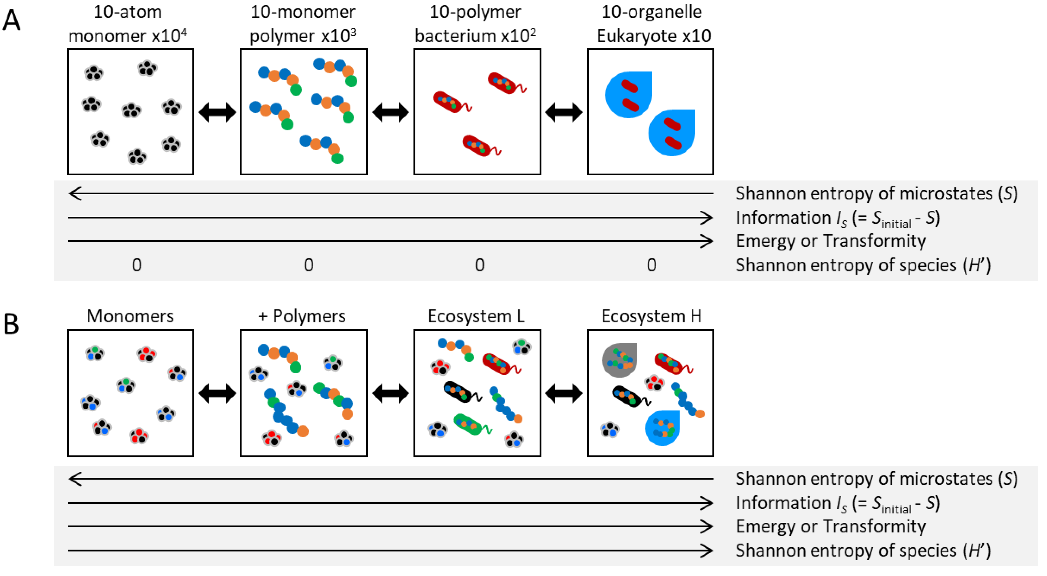
Information Dynamics in Living Systems: Macroscopic and Microscopic Perspectives
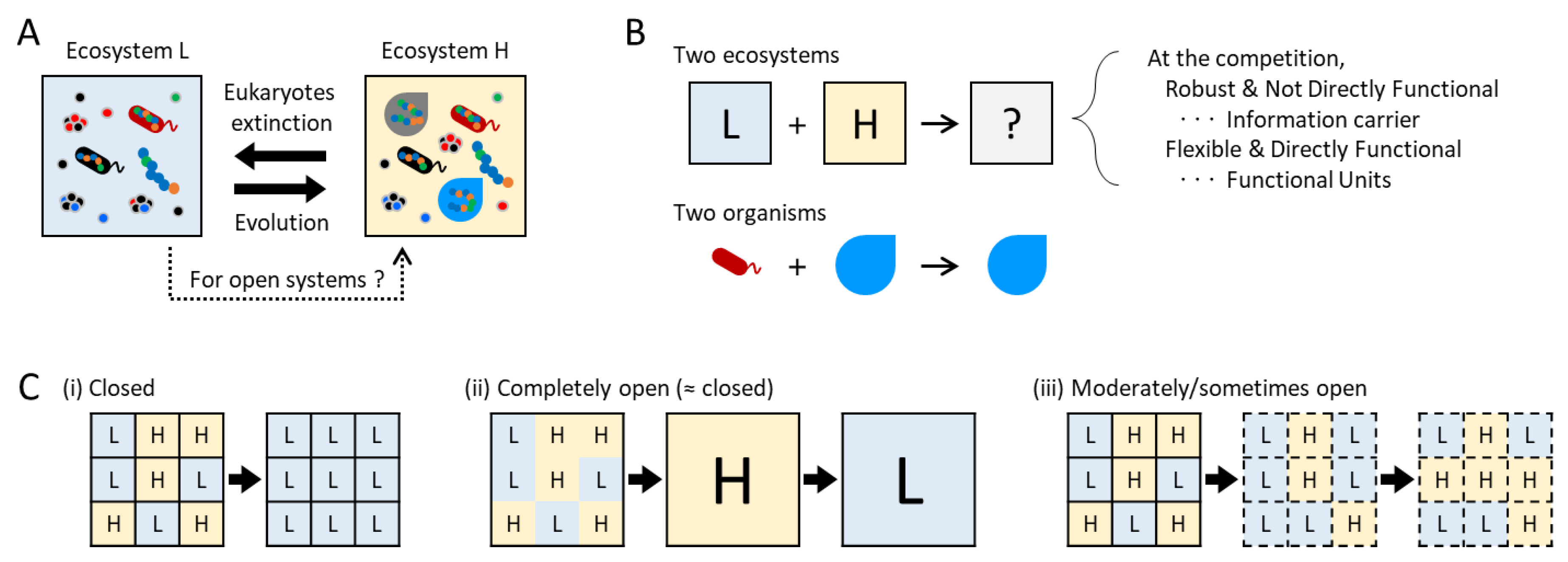
Diversity and Information Dynamics in Ecosystems: Necessity of Adaptability
Mechanism for Information Increase and Identifying Information Carriers in Ecosystems
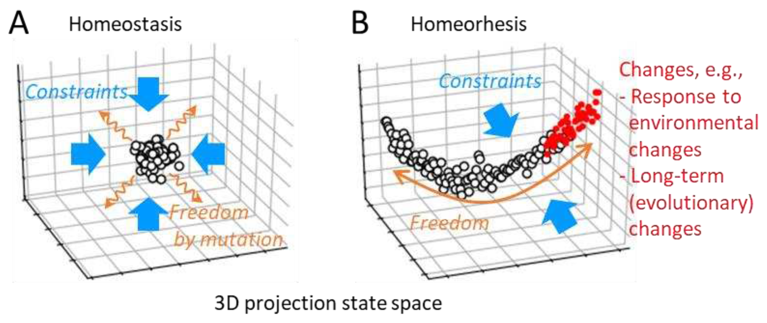
Freedom and Constraints, Homeostasis and Homeorhesis
Using Experimental Ecosystems as a Phenomenological Approach
Experiments in This Study
2. Materials and Methods
Microorganisms
Microcosm Experiments
Measurements
3. Results and Discussion
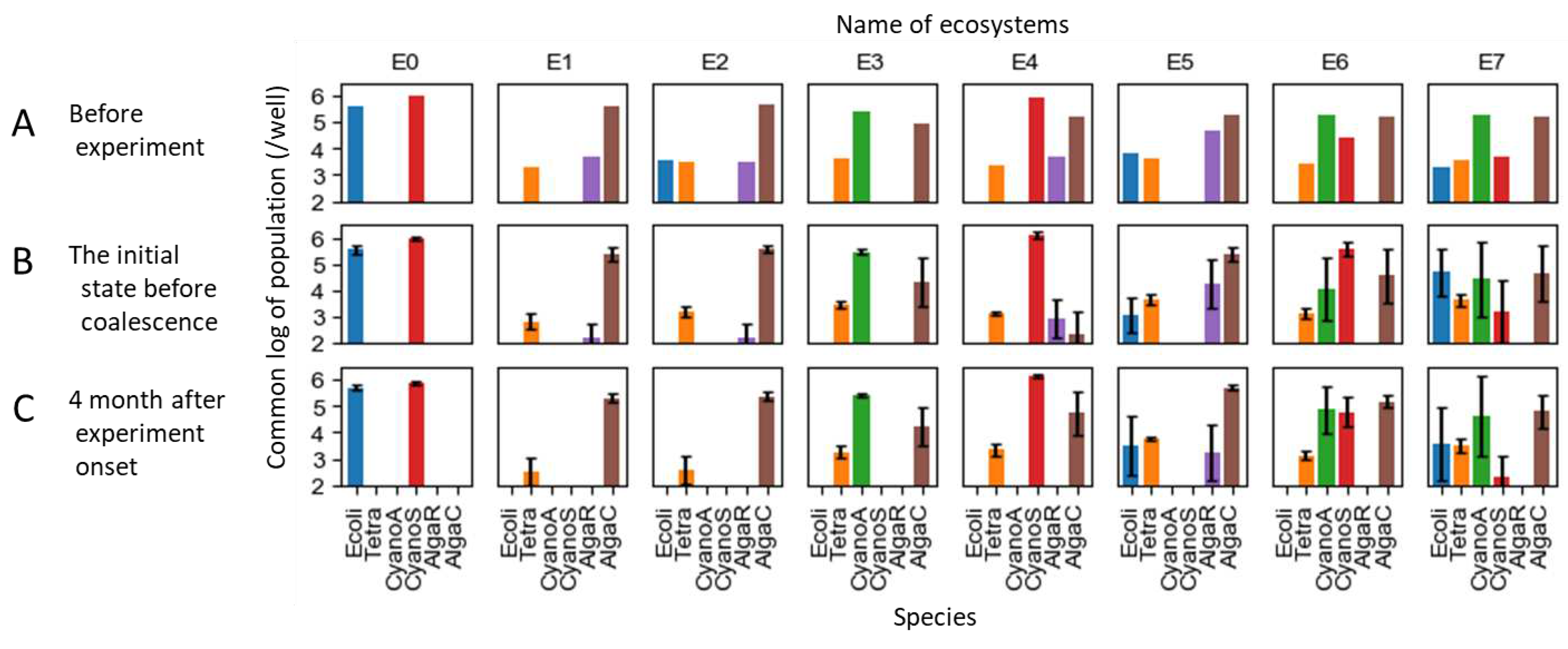
Ecosystems Used as Initial State
Ecosystem Coalescence Experiments for Investigating Competitive Stability and Information Carrier
Ecosystem Constraints for Investigating Dominant Mode Hypothesis
4. Conclusion
Author Contributions
Acknowledgments
References
- Conrad, M. Adaptability: The significance of variability from molecule to ecosystem; Springer: 1983.
- England, J.L. Dissipative adaptation in driven self-assembly. Nat Nanotechnol 2015, 10, 919–923. [Google Scholar] [CrossRef] [PubMed]
- Odum, E.P.; Barrett, G.W. Fundamentals of ecology, 5th ed.; Thomson Brooks/Cole: Belmont, CA, 2005. [Google Scholar]
- May, R.M. Will a Large Complex System Be Stable. Nature 1972, 238, 413. [Google Scholar] [CrossRef] [PubMed]
- Kondoh, M. Foraging adaptation and the relationship between food-web complexity and stability. Science 2003, 299, 1388–1391. [Google Scholar] [CrossRef] [PubMed]
- Wilmers, C.C.; Sinha, S.; Brede, M. Examining the effects of species richness on community stability: an assembly model approach. Oikos 2002, 99, 363–367. [Google Scholar] [CrossRef]
- Nature. Why interdisciplinary research matters. Nature 2015, 525, 305. [CrossRef] [PubMed]
- Cover, T.M.; Thomas, J.A. Elements of information theory second edition solutions to problems. Internet Access 2006, 19–20. [Google Scholar]
- Seifert, U. Stochastic thermodynamics, fluctuation theorems and molecular machines. Reports on progress in physics 2012, 75, 126001. [Google Scholar] [CrossRef] [PubMed]
- Sagawa, T. Second law, entropy production, and reversibility in thermodynamics of information. Energy Limits in Computation: A Review of Landauer’s Principle, Theory and Experiments, 2019; 101–139. [Google Scholar]
- Lairez, D. Thermodynamical versus logical irreversibility\: a concrete objection to Landauer’s principle. arXiv preprint arXiv:2301.07026, arXiv:2301.07026 2023.
- Chao, A.; Chiu, C.-H.; Jost, L. Phylogenetic diversity measures and their decomposition: a framework based on Hill numbers. Biodiversity Conservation and Phylogenetic Systematics 2016, 14, 141–172. [Google Scholar]
- Shannon, C.E. A mathematical theory of communication. The Bell system technical journal 1948, 27, 379–423. [Google Scholar] [CrossRef]
- Ito, S.; Sagawa, T. Maxwell’s demon in biochemical signal transduction with feedback loop. Nat Commun 2015, 6, 7498. [Google Scholar] [CrossRef]
- England, J.L. Statistical physics of self-replication. The Journal of chemical physics 2013, 139. [Google Scholar] [CrossRef] [PubMed]
- Takeuchi, N.; Kaneko, K. The origin of the central dogma through conflicting multilevel selection. Proceedings of the Royal Society B 2019, 286, 20191359. [Google Scholar] [CrossRef]
- Eigen, M. Selforganization of matter and the evolution of biological macromolecules. Naturwissenschaften 1971, 58, 465–523. [Google Scholar] [CrossRef]
- Kobayashi, I.; Sasa, S.-i. Characterizing the asymmetry in hardness between synthesis and destruction of heteropolymers. Physical Review Letters 2022, 128, 247801. [Google Scholar] [CrossRef]
- Matsubara, Y.J.; Kaneko, K. Kinetic selection of template polymer with complex sequences. Physical review letters 2018, 121, 118101. [Google Scholar] [CrossRef] [PubMed]
- Odum, E.P. The Strategy of Ecosystem Development: An understanding of ecological succession provides a basis for resolving man’s conflict with nature. Science 1969, 164, 262–270. [Google Scholar] [CrossRef]
- Yamagishi, J.F.; Saito, N.; Kaneko, K. Adaptation of metabolite leakiness leads to symbiotic chemical exchange and to a resilient microbial ecosystem. PLoS Comp. Biol. 2021, 17. [Google Scholar] [CrossRef] [PubMed]
- Elton, C.S. The ecology of invasions by animals and plants; Springer New York: 1958.
- Darwin, C. The Origin of Species by Means of Natural Selection, reprint of 6th edition. New York: The Modern Library 1872, 386.
- Hosoda, K.; Suzuki, S.; Yamauchi, Y.; Shiroguchi, Y.; Kashiwagi, A.; Ono, N.; Mori, K.; Yomo, T. Cooperative adaptation to establishment of a synthetic bacterial mutualism. PLoS One 2011, 6, e17105. [Google Scholar] [CrossRef]
- Braun, E. The unforeseen challenge: from genotype-to-phenotype in cell populations. Reports on Progress in Physics 2015, 78, 036602. [Google Scholar] [CrossRef]
- Goodfellow, I.; Bengio, Y.; Courville, A. Deep learning; MIT press: 2016.
- Murata, T.; Hamada, T.; Shimokawa, T.; Tanifuji, M.; Yanagida, T. Stochastic process underlying emergent recognition of visual objects hidden in degraded images. PLoS One 2014, 9, e115658. [Google Scholar] [CrossRef] [PubMed]
- Hosoda, K.; Seno, S.; Murata, T. Simulating Reaction Time for Eureka Effect in Visual Object Recognition Using Artificial Neural Network. IIAI Letters on Informatics and Interdisciplinary Research 2023, 3. [Google Scholar] [CrossRef]
- Hosoda, K.; Nishida, K.; Seno, S.; Mashita, T.; Kashioka, H.; Ohzawa, I. It’s DONE: Direct ONE-shot learning with quantile weight imprinting. 2022; arXiv:2204.13361.
- Power, D.A.; Watson, R.A.; Szathmáry, E.; Mills, R.; Powers, S.T.; Doncaster, C.P.; Czapp, B. What can ecosystems learn? Expanding evolutionary ecology with learning theory. Biology direct 2015, 10, 1–24. [Google Scholar] [CrossRef] [PubMed]
- Friston, K.J. The free-energy principle: a unified brain theory? Nature Reviews Neuroscience 2010, 11, 127–138. [Google Scholar] [CrossRef] [PubMed]
- Ulanowicz, R.E. The balance between adaptability and adaptation. BioSyst. 2002, 64, 13–22. [Google Scholar] [CrossRef] [PubMed]
- Waddington, C.H. The Strategy of the Genes. A Discussion of Some Aspects of Theoretical Biology; George Allen & Unwin, Ltd.: 1957.
- Cannon, W.B. Physiological regulation of normal states: some tentative postulates concerning biological homeostatics. Ses Amis, ses Colleges, ses Eleves 1926.
- Furusawa, C.; Kaneko, K. Formation of dominant mode by evolution in biological systems. Physical Review E 2018, 97, 042410. [Google Scholar] [CrossRef]
- Marconi, U.M.B.; Puglisi, A.; Rondoni, L.; Vulpiani, A. Fluctuation–dissipation: response theory in statistical physics. Physics reports 2008, 461, 111–195. [Google Scholar] [CrossRef]
- Kaneko, K. Phenotypic plasticity and robustness: evolutionary stability theory, gene expression dynamics model, and laboratory experiments. In Evolutionary systems biology, Springer: 2012; pp. 249–278.
- Maeda, T.; Iwasawa, J.; Kotani, H.; Sakata, N.; Kawada, M.; Horinouchi, T.; Sakai, A.; Tanabe, K.; Furusawa, C. High-throughput laboratory evolution reveals evolutionary constraints in Escherichia coli. Nat Commun 2020, 11, 5970. [Google Scholar] [CrossRef]
- Gao, J.; Barzel, B.; Barabási, A.-L. Universal resilience patterns in complex networks. Nature 2016, 530, 307–312. [Google Scholar] [CrossRef]
- Tu, C.Y.; D’Odorico, P.; Suweis, S. Dimensionality reduction of complex dynamical systems. Iscience 2021, 24. [Google Scholar] [CrossRef]
- Sadtler, P.T.; Quick, K.M.; Golub, M.D.; Chase, S.M.; Ryu, S.I.; Tyler-Kabara, E.C.; Yu, B.M.; Batista, A.P. Neural constraints on learning. Nature 2014, 512, 423–426. [Google Scholar] [CrossRef]
- Abbaspourazad, H.; Choudhury, M.; Wong, Y.T.; Pesaran, B.; Shanechi, M.M. Multiscale low-dimensional motor cortical state dynamics predict naturalistic reach-and-grasp behavior. Nat Commun 2021, 12, 607. [Google Scholar] [CrossRef]
- Csete, M.; Doyle, J. Bow ties, metabolism and disease. Trends Biotechnol. 2004, 22, 446–450. [Google Scholar] [CrossRef] [PubMed]
- Hinton, G.E.; Salakhutdinov, R.R. Reducing the dimensionality of data with neural networks. Science 2006, 313, 504–507. [Google Scholar] [CrossRef]
- Struhl, K. From E. coli to elephants. Nature 2002, 417, 22–23. [Google Scholar] [CrossRef]
- Taub, F.B. A Biological Model of a Freshwater Community - a Gnotobiotic Ecosystem. Limnol. Oceanogr. 1969, 14, 136. [Google Scholar] [CrossRef]
- Beyers, R.J.; Odum, H.T. Ecological microcosms; Springer-Verlag: New York, 1993. [Google Scholar]
- Tilman, D.; Wedin, D.; Knops, J. Productivity and sustainability influenced by biodiversity in grassland ecosystems. Nature 1996, 379, 718–720. [Google Scholar] [CrossRef]
- Isbell, F.; Calcagno, V.; Hector, A.; Connolly, J.; Harpole, W.S.; Reich, P.B.; Scherer-Lorenzen, M.; Schmid, B.; Tilman, D.; van Ruijven, J.; et al. High plant diversity is needed to maintain ecosystem services. Nature 2011, 477, 199–U196. [Google Scholar] [CrossRef]
- Naeem, S.; Thompson, L.J.; Lawler, S.P.; Lawton, J.H.; Woodfin, R.M. Declining biodiversity can alter the performance of ecosystems. Nature 1994, 368, 734–737. [Google Scholar] [CrossRef]
- Naeem, S.; Li, S.B. Consumer species richness and autotrophic biomass. Ecology 1998, 79, 2603–2615. [Google Scholar] [CrossRef]
- Benton, T.G.; Solan, M.; Travis, J.M.J.; Sait, S.M. Microcosm experiments can inform global ecological problems. Trends Ecol. Evol. 2007, 22, 516–521. [Google Scholar] [CrossRef]
- Hosoda, K.; Seno, S.; Murakami, N.; Matsuda, H.; Osada, Y.; Kamiura, R.; Kondoh, M. Synthetic model ecosystem of 12 cryopreservable microbial species allowing for a noninvasive approach. bioRxiv, 2023. [Google Scholar] [CrossRef]
- Rillig, M.C.; Antonovics, J.; Caruso, T.; Lehmann, A.; Powell, J.R.; Veresoglou, S.D.; Verbruggen, E. Interchange of entire communities: microbial community coalescence. Trends Ecol. Evol. 2015, 30, 470–476. [Google Scholar] [CrossRef] [PubMed]
- Diaz-Colunga, J.; Lu, N.; Sanchez-Gorostiaga, A.; Chang, C.-Y.; Cai, H.S.; Goldford, J.E.; Tikhonov, M.; Sánchez, Á. Top-down and bottom-up cohesiveness in microbial community coalescence. Proceedings of the National Academy of Sciences 2022, 119, e2111261119. [Google Scholar] [CrossRef]
- Chuang, J.S.; Frentz, Z.; Leibler, S. Homeorhesis and ecological succession quantified in synthetic microbial ecosystems. P Natl Acad Sci USA 2019, 116, 14852–14861. [Google Scholar] [CrossRef] [PubMed]
- Hekstra, D.R.; Leibler, S. Contingency and Statistical Laws in Replicate Microbial Closed Ecosystems. Cell 2012, 149, 1164–1173. [Google Scholar] [CrossRef] [PubMed]
- Louca, S.; Jacques, S.M.; Pires, A.P.; Leal, J.S.; Srivastava, D.S.; Parfrey, L.W.; Farjalla, V.F.; Doebeli, M. High taxonomic variability despite stable functional structure across microbial communities. Nat Ecol Evol 2016, 1, 0015. [Google Scholar] [CrossRef]
- Goldford, J.E.; Lu, N.; Bajić, D.; Estrela, S.; Tikhonov, M.; Sanchez-Gorostiaga, A.; Segrè, D.; Mehta, P.; Sanchez, A. Emergent simplicity in microbial community assembly. Science 2018, 361, 469–474. [Google Scholar] [CrossRef] [PubMed]
- Hosoda, K.; Tsuda, S.; Kadowaki, K.; Nakamura, Y.; Nakano, T.; Ishii, K. Population-reaction model and microbial experimental ecosystems for understanding hierarchical dynamics of ecosystems. BioSyst. 2016, 140, 28–34. [Google Scholar] [CrossRef] [PubMed]
- Momeni, B.; Chen, C.-C.; Hillesland, K.L.; Waite, A.; Shou, W. Using artificial systems to explore the ecology and evolution of symbioses. Cell. Mol. Life Sci. 2011, 68, 1353–1368. [Google Scholar] [CrossRef] [PubMed]
- Tenaillon, O.; Barrick, J.E.; Ribeck, N.; Deatherage, D.E.; Blanchard, J.L.; Dasgupta, A.; Wu, G.C.; Wielgoss, S.; Cruveiller, S.; Medigue, C.; et al. Tempo and mode of genome evolution in a 50,000-generation experiment. Nature 2016, 536, 165. [Google Scholar] [CrossRef]
- Blount, Z.D.; Lenski, R.E.; Losos, J.B. Contingency and determinism in evolution: Replaying life’s tape. Science 2018, 362. [Google Scholar] [CrossRef]
- Nakajima, T.; Sano, A.; Matsuoka, H. Auto-/heterotrophic endosymbiosis evolves in a mature stage of ecosystem development in a microcosm composed of an alga, a bacterium and a ciliate. BioSyst. 2009, 96, 127–135. [Google Scholar] [CrossRef]
- Germond, A.; Kunihiro, T.; Inouhe, M.; Nakajima, T. Physiological changes of a green alga (Micractinium sp.) involved in an early-stage of association with Tetrahymena thermophila during 5-year microcosm culture. BioSyst. 2013, 114, 164–171. [Google Scholar] [CrossRef] [PubMed]
- Nakajima, T.; Fujikawa, Y.; Matsubara, T.; Karita, M.; Sano, A. Differentiation of a free-living alga into forms with ecto- and endosymbiotic associations with heterotrophic organisms in a 5-year microcosm culture. BioSyst. 2015, 131, 9–21. [Google Scholar] [CrossRef] [PubMed]
- Nakajima, T. Symbiogenesis is driven through hierarchical reorganization of an ecosystem under closed or semi-closed conditions. BioSyst. 2021, 205. [Google Scholar] [CrossRef] [PubMed]
- Allen, M.M. Simple conditions for growth of unicellular blue-green algae on plates1, 2. J. Phycol. 1968, 4, 1–4. [Google Scholar] [CrossRef] [PubMed]
- Bertani, G. Studies on Lysogenesis.1. The Mode of Phage Liberation by Lysogenic Escherichia-Coli. J. Bacteriol. 1951, 62, 293–300. [Google Scholar] [CrossRef]
- Redmon, J.; Farhadi, A. YOLOv3: An Incremental Improvement. 2018; arXiv:1804.02767.
- Hosoda, K.; Habuchi, M.; Suzuki, S.; Miyazaki, M.; Takikawa, G.; Sakurai, T.; Kashiwagi, A.; Sueyoshi, M.; Matsumoto, Y.; Kiuchi, A. Adaptation of a cyanobacterium to a biochemically rich environment in experimental evolution as an initial step toward a chloroplast-like state. PloS one 2014, 9, e98337. [Google Scholar] [CrossRef] [PubMed]
- Azuma, Y.; Tsuru, S.; Habuchi, M.; Takami, R.; Takano, S.; Yamamoto, K.; Hosoda, K. Synthetic symbiosis between a cyanobacterium and a ciliate toward novel chloroplast-like endosymbiosis. Scientific Reports 2023, 13, 6104. [Google Scholar] [CrossRef] [PubMed]
- Tan, X.P.; Shan, Y.Q.; Wang, X.; Liu, R.P.; Yao, Y.L. Comparison of the predictive ability of spectral indices for commonly used species diversity indices and Hill numbers in wetlands. Ecol. Indicators 2022, 142. [Google Scholar] [CrossRef]
- Faith, J.J.; Guruge, J.L.; Charbonneau, M.; Subramanian, S.; Seedorf, H.; Goodman, A.L.; Clemente, J.C.; Knight, R.; Heath, A.C.; Leibel, R.L. The long-term stability of the human gut microbiota. Science 2013, 341, 1237439. [Google Scholar] [CrossRef]
- Payton, I.J.; Fenner, M.; Lee, W.G. Keystone species: the concept and its relevance for conservation management in New Zealand; Department of Conservation Wellington: 2002.
| Species | Abbreviation | Classification | Functional group | Shape, approx. vol. | |
| #0 | Escherichia coli | Ecoli | Proteobacteria | Decomposer | Rod, 1 μm3 |
| #1 | Tetrahymena thermophila | Tetra | Ciliophora | Consumer | Oval, 104 μm3 |
| #2 | Anabaenopsis circularis | CyanoA | Cyanobacteria | Producer | Filamentous, 103 μm3 |
| #3 | Synechocystis sp. 6803 | CyanoS | Cyanobacteria | Producer | Spherical, 10 μm3 |
| #4 | Raphidocelis subcapitata | AlgaR | Chlorophyta | Producer | Crescent, 102 μm3 |
| #5 | Chlorella vulgaris | AlgaC | Chlorophyta | Producer | Spherical, 102 μm3 |
Disclaimer/Publisher’s Note: The statements, opinions and data contained in all publications are solely those of the individual author(s) and contributor(s) and not of MDPI and/or the editor(s). MDPI and/or the editor(s) disclaim responsibility for any injury to people or property resulting from any ideas, methods, instructions or products referred to in the content. |
© 2023 by the authors. Licensee MDPI, Basel, Switzerland. This article is an open access article distributed under the terms and conditions of the Creative Commons Attribution (CC BY) license (http://creativecommons.org/licenses/by/4.0/).


