Preprint
Article

Experimental Research on Avoidance Obstacle Control for Mobile Robots Using Q-Learning (QL) and Deep Q-Learning (DQL) Algorithms in Dynamic Environments

Altmetrics

Downloads

92

Views

46

Comments

0

A peer-reviewed article of this preprint also exists.

This version is not peer-reviewed

Submitted:

07 November 2023

Posted:

07 November 2023

You are already at the latest version

Alerts
Abstract
This paper presents experimental results of static and dynamic obstacle avoidance methods for a two-wheel mobile robot with independent control using a deep Q-learning (DQL) reinforcement learning algorithm. This is an alternative method that combines the Q-learning (QL) algorithm with a neural network. Neural networks in the DQL algorithm act as Q matrix table approximators for each pair (State - Action). The effectiveness of the proposed solution was verified through simulations, programming, and experimentation. This DQL algorithm is compared to the QL algorithm. First, the mobile robot communicated with the control script using the robot operating system (ROS). The mobile robot is code programmed using a Python in the ROS operating system combined with the DQL controller in Gazebo software. The mobile robot then performed experiments in a workshop with many different experimental scenarios. This DQL controller is improved in term of the computation time, convergence time, planning trajectory accuracy, and obstacles avoidance. Therefore, the DQL controller solved the path optimization problems for mobile robots better than the Q-learning controller.
Keywords: 
Subject: Engineering  -   Control and Systems Engineering

1. Introduction

Mobile robots have become an indispensable part of social development. It takes on dangerous tasks that are difficult for humans, such as search and rescue, support in epidemic areas, and exploration of the distant planets. Therefore, the design of mobile robots requires planning the trajectory of the robot as acritical factor [1]. This trajectory planning will focus on creating the shortest distance, the least time, the most energy saving, and avoiding all obstacles when moving to the target [2]. Mobile robots include global path planning, local path planning, static path planning, and dynamic path planning [3,4].
Researchers have recently published more trajectory-planning studies on mobile robots to avoid obstacles in the operating environment. This is a linear, nonlinear, and intelligent algorithm. In [5], mobile robots used a magnetic field (APF) algorithm to plan the path. In another study, the checkerboard method used a simulation algorithm many times to find the optimal trajectory for mobile robots [6]. In addition, there are popular pathfinding algorithms for static obstacle avoidance, such as the A* algorithm [7], D algorithm [8], DWA algorithm [9], random tree algorithm (RRT) [10], genetic algorithm (GA) [11], optimization particle swarm (PSO) [12], ant colony optimization [13], gravity search algorithm (GSA) [14] pigeon-inspired optimization [15], the robot is moved according to the trajectories set based on the PID-FLC controller [16], and intelligent control for mobile robots based on fuzzy logic controller [17]. By analyzing the research results above, mobile robots only have fast, accurate opera in the static environment (when the environment has complete knowledge of the area). The mobile robot was able to adjust its movement speed and trajectory to avoid obstacles. However, orbital navigation planning for mobile robots is effective in dynamic environments (when the environment is complex with many variabilities) [18]. Therefore, AI algorithms are suggested ways for planning the trajectory mobile robots in this dynamic environment, such as the GA-fuzzy method [19], ANFIS [20], reinforcement learning (RL,) and machine learning (ML). With this AI algorithm, the trajectory for mobile robots can be trained and updated online in real time [21].
Based on a previous study [22], scientists have extensively used the RL algorithm in entertainment games and information technology. However, many researchers have applied this algorithm's optimal feature, simple controller design, and orbital navigation planning for mobile robots [23,24]. However, the RL algorithm only slightly improves a little regarding the path and increases the convergence computation time. Following the paper [25,26,27], the Q-Learning (QL) algorithm plans the trajectory of the mobile robot by learning from previous observations of the environment. The QL algorithm improved accelerated computation and convergence. However, the QL algorithm calculates the Q values of states to make the action values of neural network lager. Because the QL algorithm had to access all the action-state pairs in complex, dynamic environments, it took a lot of time to plan the trajectory for the mobile robot. Therefore, many studies have proposed different solutions to the reduced disadvantages of traditional QL algorithms. Nakashima and Ishibashi [28] used a fuzzy set to moderate the appropriate Q-value initialization, which accelerates the convergence. In another study, Jiang and Xin [29] presented a QL algorithm that generates undefined state variables using a new technique for continuous space division and learning planning in an unknowable dynamic environment. Additionally, scientists have suggested an integrated learning strategy based on spatial allocation to hasten the learning process. When paired with the QL method, the State-Action-Reward-State-Action (SARSA) technique allowed Wang et al. [30] to achieve convergence quickly, and the findings demonstrated that the learning time decreased. Das et al. [31] created an alternative to QL to solve the problem of convergence rate. To update the Q table in a more organized manner with less time and space complexity, Goswami et al. [32,33] updated the basic QL algorithm. The Q values are retained in the Q table at the values with the best action in each state. This saves a lot of complicated time because it takes only a short time to obtain the Q values. Scientists created a separate field for the operation of each table. Several QL algorithms reduce the computation and convergence times of the planning trajectories for mobile robots in complex and, dynamic environments. However, to improve navigation control in both static and dynamic environments for mobile robots, this study developed a Deep Q-Learning (DQL) algorithm. DQL has neural networks that act as Q-value approximators for each pair (state-action).
The paper has some contributions below.
Studies on the complexity of mobile robot paths based on the DQL algorithm using case experiments.
Simulation and experimental results for robots using the DQL algorithm compared to the QL algorithm have demonstrated the efficiency and superiority of the proposed algorithm in terms of (1) the proposed DQL can quickly and safely generate optimal and near-optimal (short) paths; (2) the DQL approach is deterministic and requires a few milliseconds to compute a good solution in terms of length and safety; and (3) DQL based algorithms are non-deterministic and lack a good trade-off between convergence speed and path length. (4) The proposed DQL performance was improved compared with the performance of the latest related work. Finally, (5) the suggested DQL increased the route quality with respect to the length, computation time, and robot safety.
The remainder of this paper is organized as follow. The path planning control problems for mobile robots are in the described in section. The mathematical modeling of the operating system for a mobile robot is described in section two. The design of the optimal path for mobile robots using the DQL algorithm is described in section three. Finally, the effectiveness of the solution is tested, compared, and analyzed through simulations and experiments with the QL algorithm in section four.

2. Mathematical Modeling of Operating System for a Mobile Robot

2.1. Obstacle Modeling in Mobile Robot Operating enviroment

The obstacle model is built on a rectangular box. Among the static and dynamic path optimization techniques that collect obstacle estimates, the optimal geometry allows easy estimation of any obstacle shape. The obstacles using cubes, are shown in Figure 1. Figure 1 (a) Using this geometry to plan the robot in 2D, blocks can be replaced while avoiding 3D obstacles. A realistic scene with 3D blocks (chairs, tables, etc.) is shown in Figure 1(b). A binary map of the modeled environment is shown in Figure 1(c).

2.2. Mathetical Model

The mobile robot moves from the start point start. ( x s , y s ) to the destination point target ( x T , y T ), the purpose of the robot path planning is to find the optimal path from the Start point to the Target point, this path is connected by n nodes ( N i , i = 1... n ) and ( n-1) each segment is 2 consecutive nodes connected to each other. We assume that the robot moves in an environment with m known obstacles as shown in Figure 1. Each obstacle is modeled surrounded by a rectangle with four vertices and four edges o b s _ s e g t j ( t { 1 4 } , j { 1 m } ) .
where p 1 is the bottom left corner of the rectangle. Similar to obstacles in the environment, the mobile robot is also estimated by a rectangle of four points, and their coordinates change according to the robot's current position. The mathematical equation of each segment defined by the two points ( p k , p l ) of a rectangle enclosing an obstacle is given by Eq. (1):
s e g ( p k , p l ) = { y y k = y l y k x l x k ( x x k ) M i n ( x l , x k ) x M a x ( x l , x k )
The following notations describe the indices and parameters used in the mathematical model:
n: number of nodes on the trajectory created from the starting point to the destination.
m: number of obstacles in the environment.
  • i ( i { 1... n } ) : fragment index generated by the node i and i + 1.
  • j ( j { 1... m } ) : index of the j t h obstacle in the navigation environment.
  • k , l ( k , l { 1...4 } ) : indices of the point that defines an obstacle.
  • r(r∊{1…4}): index of segment r from the rectangle approximating the mobile robot.
  • t ( t { 1...4 } ) : index of the segment t that defines the rectangle of an obstacle.
  • N i : i t h node of the path.
  • o b s j ( j { 1... m } ) : j t h obstacle.
  • p a t h _ s e g i ( N i , N i + 1 ) ( i { 1... n 1 } ) : i t h segment of the path defined by two nodes ( N i , N i + 1 ) .
  • o b s _ s e g l j ( p k , p l ) ( k , l { 1...4 } ) j ( j { 1... m } ) : l t h segment of j t h obstacle defined by two points ( p k , p l ).
  • CurrentPos: current location of the robot.
  • R o b _ s e g r ( p k , p l ) ( r , k , l { 1...4 } ) : r t h segment of the rectangle approximating the robot.
The mathematical model’s decision variables are computed as follows:
B i , t , j = { 1 i f P 1 , P 2 | { P 1 , P 1 } ( p a t h _ s e g i ) { P 1 , P 1 } ( o b s _ s e g t j ) j ( j { 1... m } , t ( t { 1...4 } ) , i ( i { 1... n } 0 O t h e r w i s e
A i , t , j = { 1 i f P 1 , P 2 | { P 1 , P 1 } ( p a t h _ s e g r ) { P 1 , P 1 } ( o b s _ s e g t j ) j ( j { 1... m } , r , t ( t { 1...4 } ) , 0 O t h e r w i s e
The objective function is to find the shortest path according to Eq. (4)
M i n i m i z e ( 1 = 1 i = n 1 ( x i + 1 x i ) 2 + ( y i + 1 y i ) 2 , { 1... n 1 } )
Equation (5) requires each node to be unique:
( x i + 1 x i ) ( y i + 1 y i ) , i { 1... n 1 }
Path segments do not overlap in the environment by Eq.(6)
i = 1 i = n 1 j = 1 j = m B i , t , j = 0 , i { 1... n } , t { 1...4 } , j { 1... m }
The way nodes for the robot to overcome obstacles are calculated by Eq.(7).
j = 1 j = m A r , t , j = 0 , r , t { 1...4 } , j { 1... m }
All variables A and B must be binary to satisfy requirement Eq. (8)
B i , t , j { 0 , 1 } , A r , t , j { 0 , 1 } i { 1... n } , r , t { 1...4 } , j { 1... m }

3. Deep Q-Learning and Q-Learning Alorithms in Path Planing for Mobile Robots

3.1. Q-Leaning

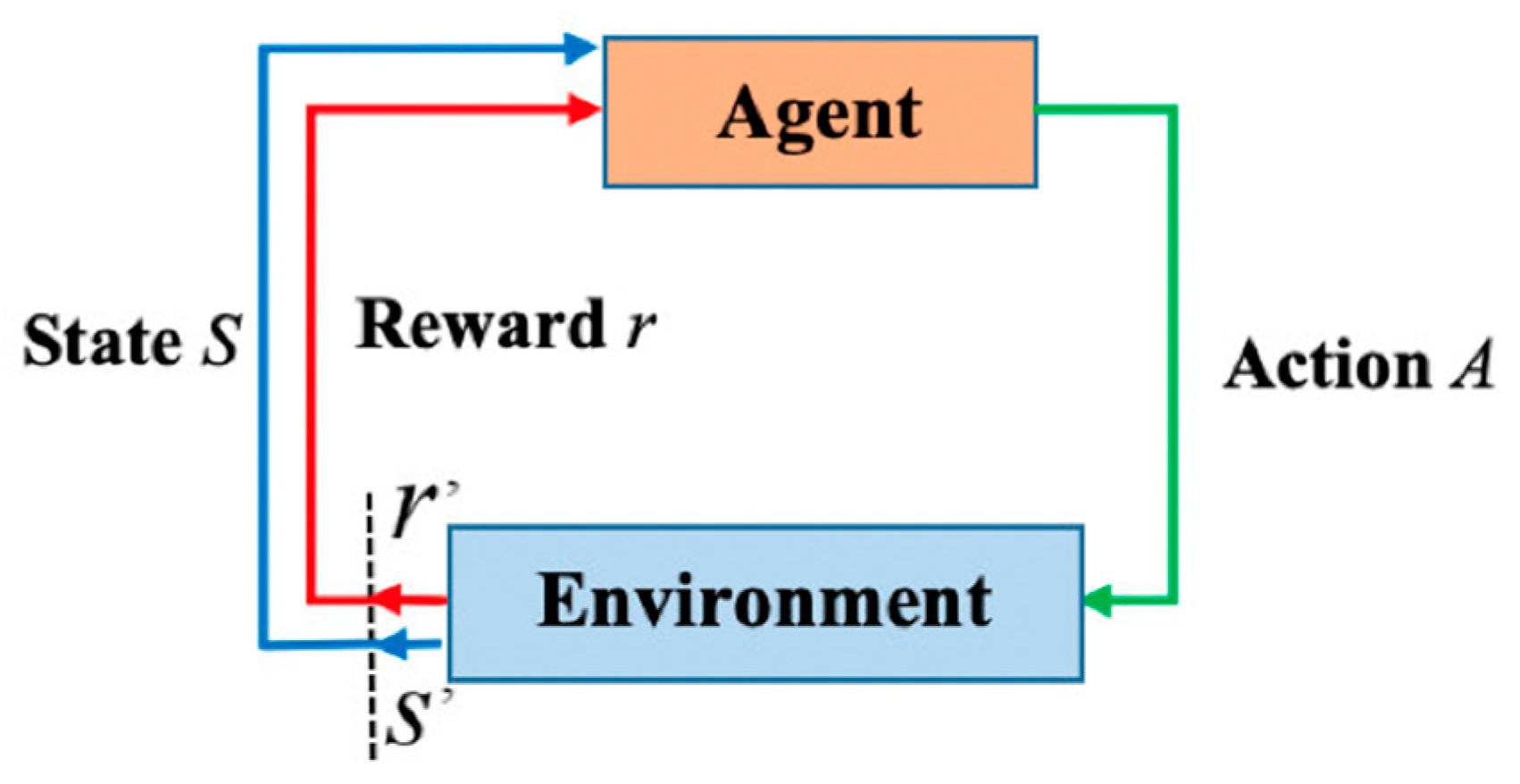
The Q-learning (QL) algorithm uses the concept of reward and punishment is created in the environment. Figure 2 illustrates how a mobile robot selects an action based on the appropriate policy, executes that action, and receives status (s) and rewards (r) from the navigation environment. A state contains the robot's current position in its workspace while optimizing paths, while an action is a movement the robot transitions from one state to another.
The Q value was built so that for robot to decide to earn the greatest reward. This is calculated as follows:
Q ( s t , a t ) = Q ( s t , a t ) + α [ r ( s t , a t ) + γ max Q a A ( s t + 1 , a ) - Q ( s t , a t ) ]
where: α represents the learning rate, γ is the discount factor, s t m a x a A Q ( s t + 1 , a ) signifies the maximum Q v a l u a among all feasible actions in the new state a t , and denotes the immediate reward/penalty earned by the agent after executing a move at state s t + 1 .
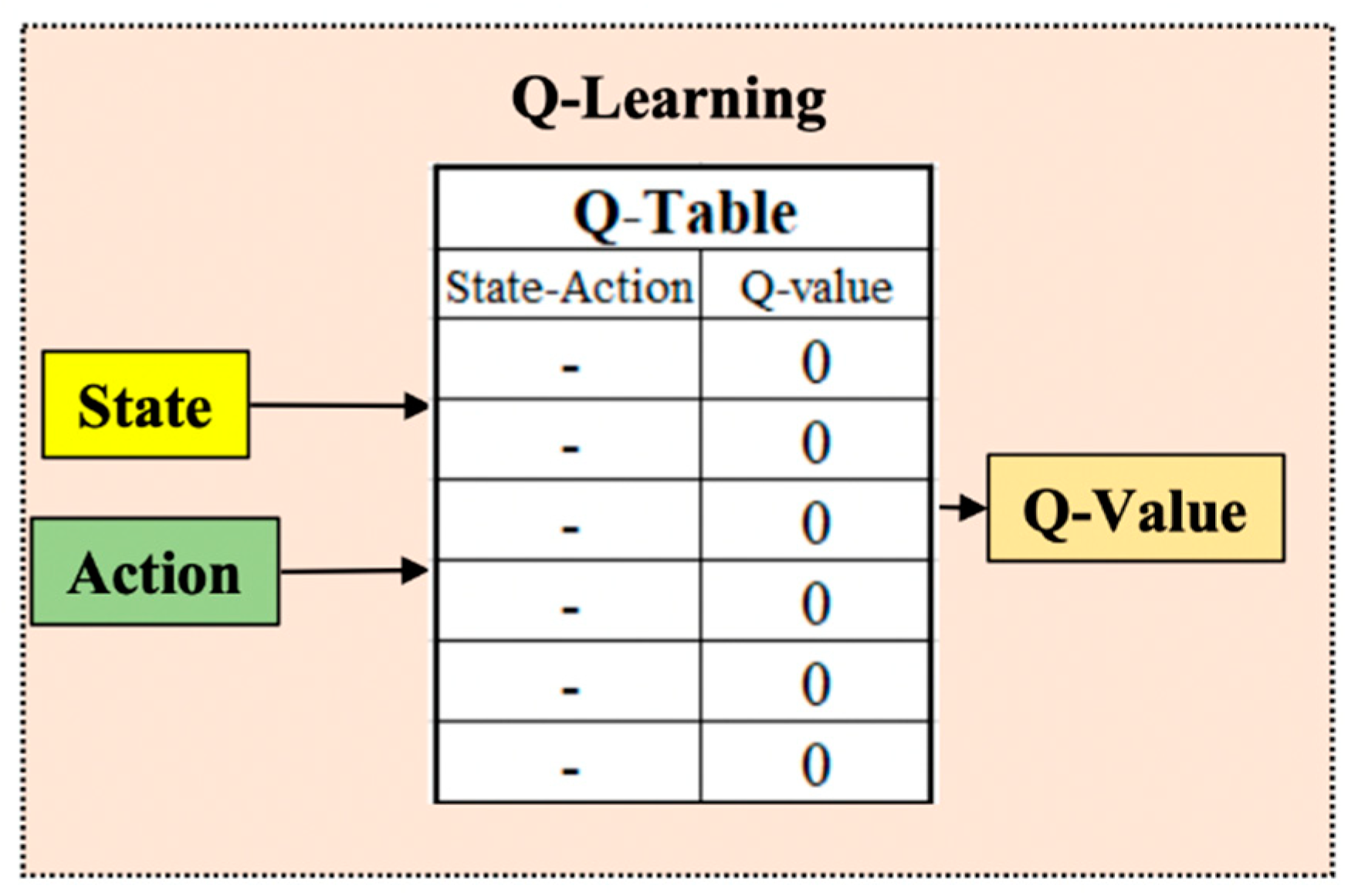
Based on Eq. (9) is state matrix – which acts as a lookup table. From there, for each state of the robot, we found the action with the most significant Q value (Figure 3).
Reinforcement learning is a random process, therefore the Q values will differ before and after the action. This is called a temporary difference.
T D ( a , s ) = r ( s t , a t ) + γ max Q a A ( s t + 1 , a ) - Q ( s t , a t )
Thus, the matrix Q ( s t , a t ) needs to update the weights based on Eq. (11):
Q t ( s t , a t ) = Q t 1 ( s t , a t ) + α T D t ( a t , s t )
where: α is an arithmetic coefficient. Through the times the robot performs actions; Q ( s , t a t ) it will gradually converge.
The programming program for the Q-learning algorithm for robot pathfinding is expressed as follows:
Algorithm 1: Classical Q-Learning algorithm begin Initialization:
Q ( s t , a ) t { 0 } , (states and 𝒎 actions)
for (each episode):
(1)
Set s t ← a random state from the states set s;
while ( s t Goal stage)
(2)
Choose a t in s t by using an adequate policy (𝜺 -greedy, etc.);
(3)
Perform action a t , and receive reward/penalty and s t + 1 ;
(4)
Update Q ( s t , a ) t using equation (9);
s t s t + 1

end-while
end-for
end
The size of the Q table increases exponentially with the number of states and actions in an environment with conditions.
In this situation, the process becomes computationally expensive and requires considerable memory to hold the Q values. Imagine a game in which each state has 1000 actions. A table with one million cells is required. Given the vast amount of computational time [31], one of the main problems when using the QL algorithm in path optimization is that accessing all the action-state pairs during the mining process is complex, which affects orbital convergence.

3.2. Deep Q-Leaning

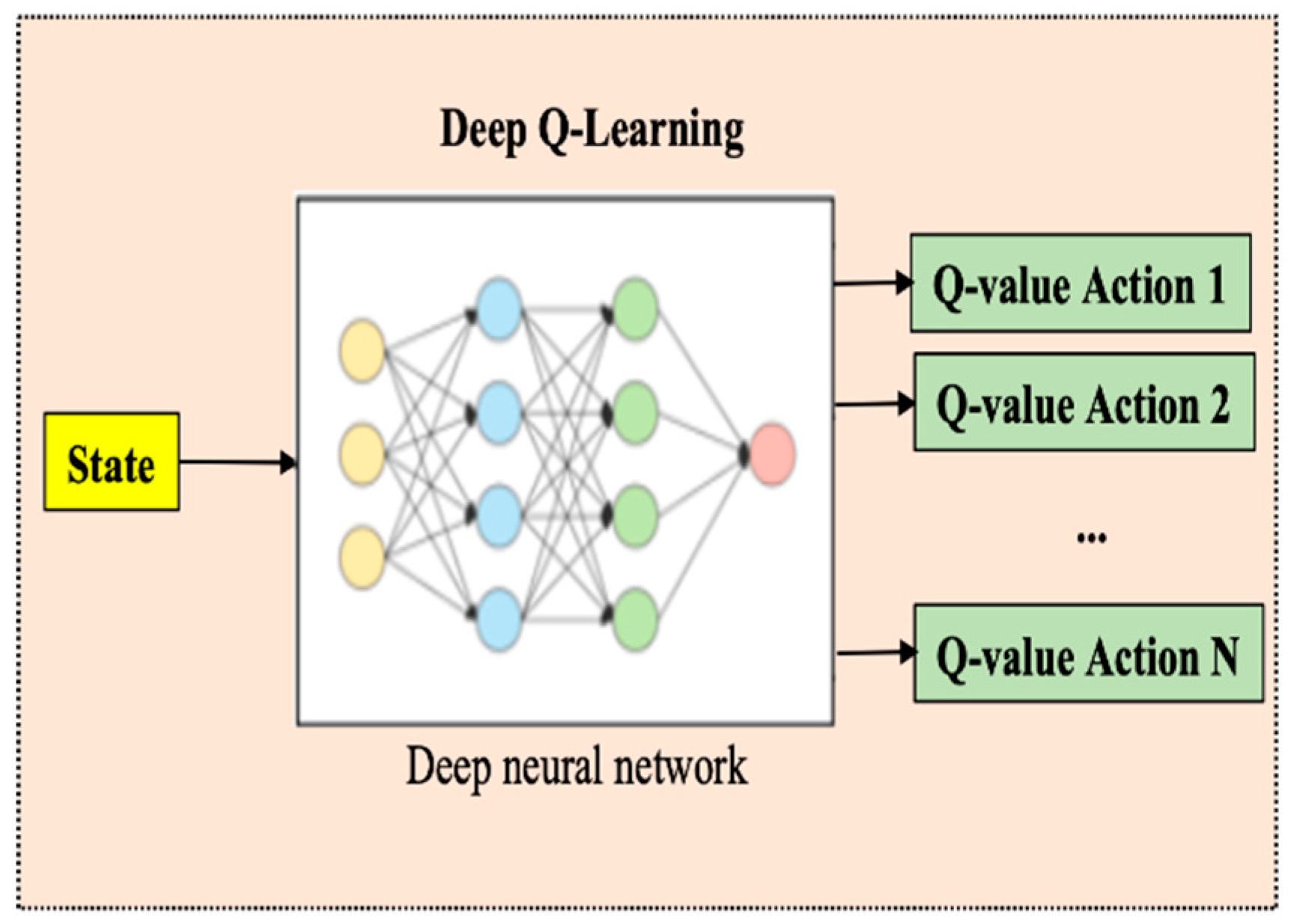
The DQL algorithm replaces the regular Q table with a neural network. Instead of mapping a (state-action) pair to a Q-value, the neural network maps the input states to (action, Q-value) pairs, as shown in Figure 4.
State evolution data were used for the neural network input, and the Q value corresponded to each separate output node of the neural network. Therefore, each predicted Q value of an individual action is in state.
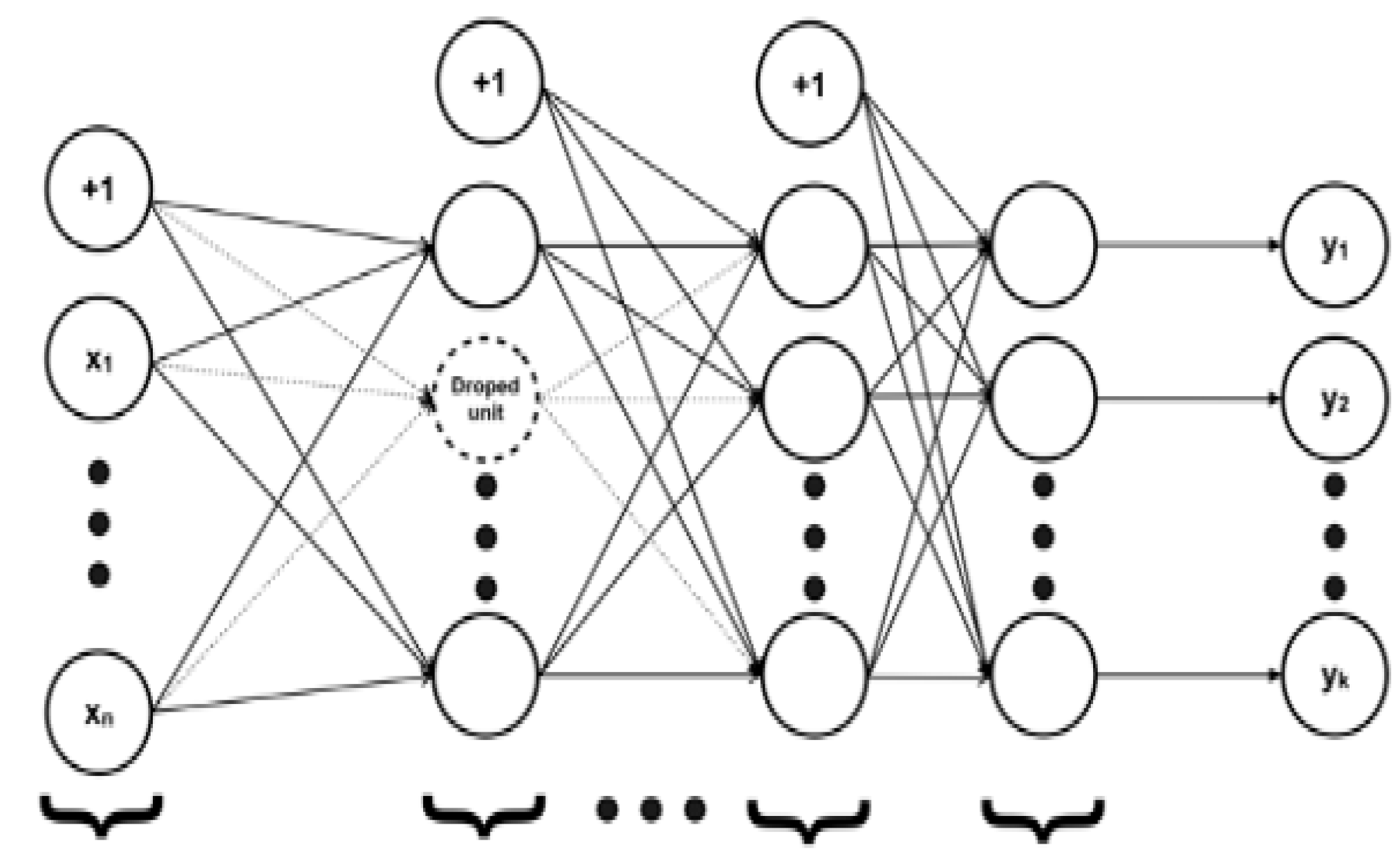
The proposed model for deep learning neural networks has four layers: one input layer, two hidden layers, and one output layer (Figure 5). There were 1856 training parameters in the first hidden layer, comprising architecture neurons that are entirely associated with 28 laser sensor inputs. Four thousand one hundred sixty parameters were trained in the second hidden layer, including 64 neurons and 64 inputs from the first.
A programming program for the DQL algorithm as follows:
Input: data X = ( x 1 , x 2 , ... , x N ) , learning factor α, discount factor, epsilon-greedy policy , robot pose, safety constraints
Output: Q ( s , a ; θ ) , states’ s є S, actions a є A, weight θ
Begin
        Initialize replay memory D to capacity N
        Initialize Q ( s , a ; θ ) with random weights
        Initialize Q ( s , a ' ; θ ' ) , with random weights
for episode = 1, M do
Randomly set the robots pose in the scenario Observe initial states of robots s
    for t = 1, T due to:
Select an action a t
        With probability select a random action a t
        Otherwise select a t = arg max a ' Q ( s t , a ' ; θ )
        Execute action a t , observer state s t + 1 , compute reward R t
Store training ( s t , a t , R t , s t + 1 ) in relay memory EASY
Sample random minibatch of transition ( s t , a t , R t , s t + 1 ) from EASY
Calculate the predicted value Q ( s j , a j ; θ )
Calculate target value for each minibatch transition
        If s t + 1 is terminal state the y j = R j
        Otherwise y j = R j + γ max a ' j Q ' ( s ' j , a ' j ; θ ' )
        Train neural networks using ( y j Q ( s j , a ; j θ ) ) 2     end for
end for
The robot makes decisions and performs actions according to the Q-based (ε-greedy) policy. A mobile robot must successfully consider more than short-term gains over the long term. Mention any prizes it might win in Class 1, Class 2, Class L -1 future class. In addition, because the environment is unpredictable, the mobile robot can never be sure to receive the same reward the following time it takes the same activities. Robot can diverge further as they advance in the future. Therefore, we employ a future discount reward in this study. The following formula is used to calculate the return on the future dilution factor at time t:
R t = r t + γ r t + 1 + γ 2 r t + 2 + ... + γ T t r T , 0 γ 1
where: r t is the direct reward, and T is the time step at which the robot action ends, the more future the reward, the less the robot considers it.
The goal of the robot is to interact with the environment by choosing actions that maximize future rewards. A technique called experience replay, in which we record the robot's experience at each time step, e t = ( s t , a t , R t , s t + 1 ) in a data set D t = { e 1 , ... , e t } which pooled over many learning cycles (episodes). at the end of the learning cycle into replay memory.
Update the weights of neural networks. First sample random transitions from replay memory D with finite memory size N. For each given transformation, the algorithm performs the following steps:
- Step 1: Transition through the neural network for the current state to obtain the predicted value Q ( s j , a ; j θ ) .
- Step 2: If the transition sampled is a collision sample, then the evaluation for this pair ( s j , a j ) is directly set as the termination reward. Otherwise, forward neural networks are performed for the next state s', the maximum overall network output is calculated, and the target for the action is computed using the Bellman equation (r + max a ' j Q ' ( s ' j , a ' j ; θ ' ) ). For all other activities, the target value is set to be the same as that initially returned in step 1.
- Step 3: The Q-learning update algorithm uses the following loss function:
L ( θ ) = 1 N i = 1 n ( y j Q ( s j , a ; j θ ) ) 2
The neural network weights were be changed using a loss function through backpropagation and stochastic gradient descent. The mobile robot stores the learned neural networks in its brain when the training is over and uses them for future testing and work.

4. Simulation and Experimental Results

This study proposes a DQL-based obstacle avoidance trajectory planning strategy for a mobile robot operating in an unexplored area using a LIDAR sensor. The LIDAR sensor acquires the distance value to the system and decides what to do next based solely on the distance of the obstacle to the mobile robot.
In this process, the unnatural acceleration or deceleration actions of the system are required during resonance. The action value frequently fluctuates, physically shocks the robot, and reduces path performance. Therefore, the action values are returned to the input in the order of the network action after being held in memory.
In addition, reinforcement learning was simulated on Robot Operating System and Gazebo simulator (ROS-GAZEBO) and experiments were conducted on actual mobile robots by scenarios and analyzing the experiment.
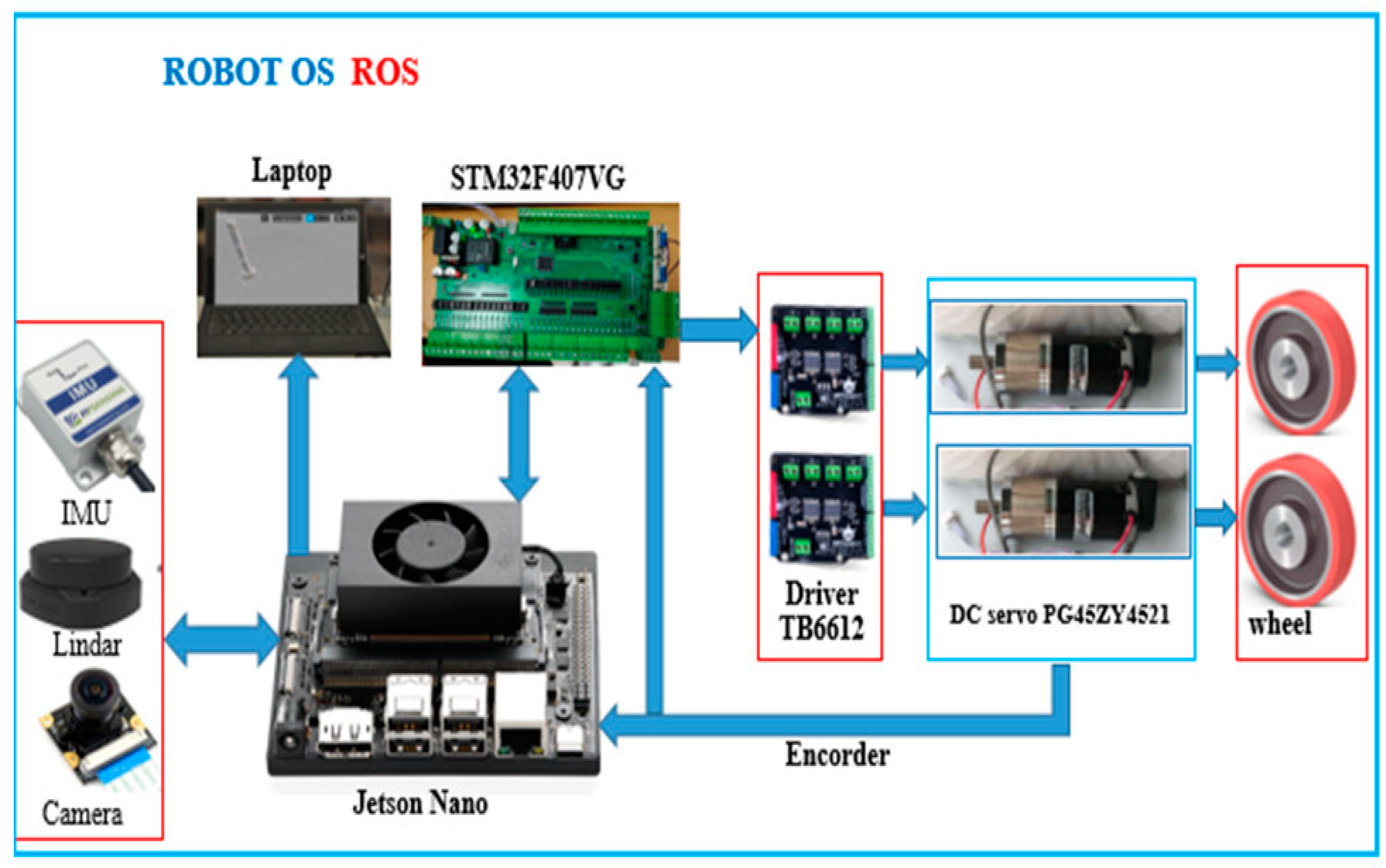
In this study a mobile robot was experimentally built with specifications and a steel body size of 70cm x 50cm x 38cm. Its 10 cm diameter wheels handle nearly any surface in the home. The two motor shafts hold 1200-tick encoders. This differential drive platform is comprehensive can rotate in place. The wheels move only on one side with two DC motors attached to the encoder. The robot was equipped with a Jetson Nano 4G embedded computer processor. ROS programming software specifications, motor encoder information, and other I/O via packets from the Jetson Nano 4G walker server all micro-control to the personal computer (PC) client and return control commands. Signals were obtained for power from the Lindar 3600 A2 sensors, camera, and Inertial Measurement Unit (IMU). ROS software provides library functions for navigation, path planning, obstacle avoidance, and many other robotic tasks. Figure 6.

4.1. Set Status for a Mobile Robot

This state is an environment that observes and describes the current position of the robot. The state size is 28, with 24 values for laser distance sensor, distance to target, and angle to target.

4.2. Set Action for a Mobile Robot

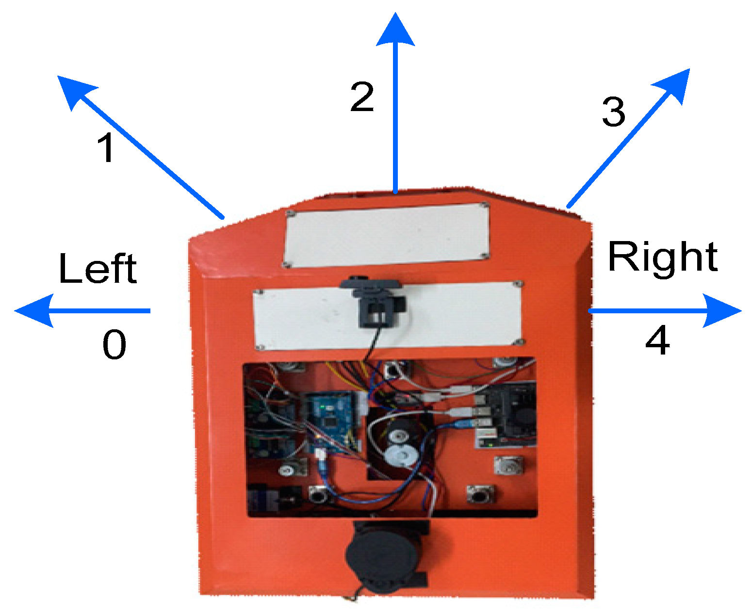
The robot could perform actions only in each state. The linear speed of the mobile robot in this situation was always 0.15 m/s. Act of determining angular rate. The authors used a mobile robot model (Figure 7) that could only perform the five possible tasks listed in Table 1:

4.3. Set Up Reward for a Mobile Robot

The mobile robot performs an action in this state. It received a reward. Reward design is crucial to learning. Reward can be either positive or negative. When the robot achieves its goal, it receives a sizeable positive compensation. When the robot collided with an obstacle, it received a large negative reward.

4.4. Parameter Setting for the Controller

Table 2. Action and Angular.
T 6000(s) Time step of 1 cycle
γ 0.99 The discount factor
α 25.10 5 Learning speed
ξ 1.0 Probability of choosing a random action
ξ reduce 0.99 Reduction rate of epsilon. When a cycle ends epsilon decreases
ξ min 0.05 Minimum stats of epsilon
Batch size sixty-four Activate a group of training templates
Train start Sixty -four Start of input training
Memory 10 6 Memory size

4.5. Simulation Results on ROS-GAZEBO

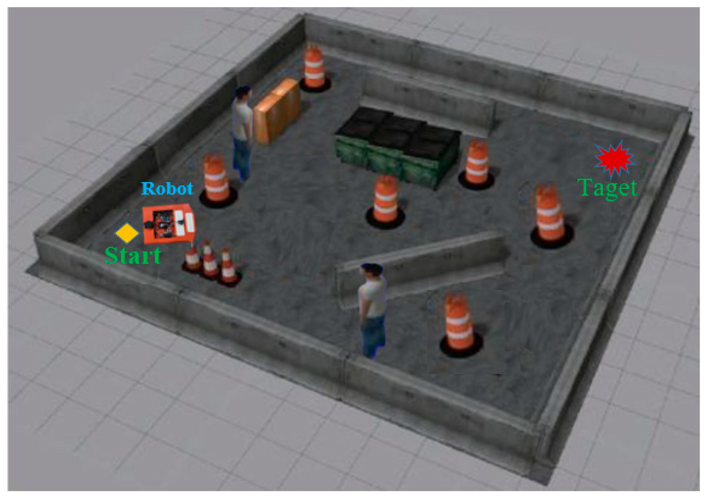
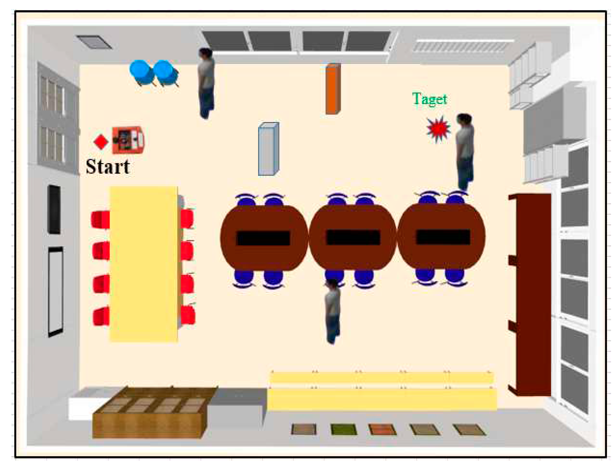
In this study, the control robot system created a scenario similar to that of a simulated factory in ROS-Gazebo to bridge the gap between the simulated environment and the natural world (Figure 8).
In this environment, various obstacles were built to test the proposed QL and DQL navigation algorithms. The territory includes walls, static blocks, mobile people, targets, and mobile robots. The mobile robot must reach the target while avoiding static and dynamic obstacles as illustrated in Figure 8
The training process for a robot can undergo several cycles. Each cycle ended when the robot acquired the target position, hit an obstacle in the path of the robot, or when the time for each cycle expired.
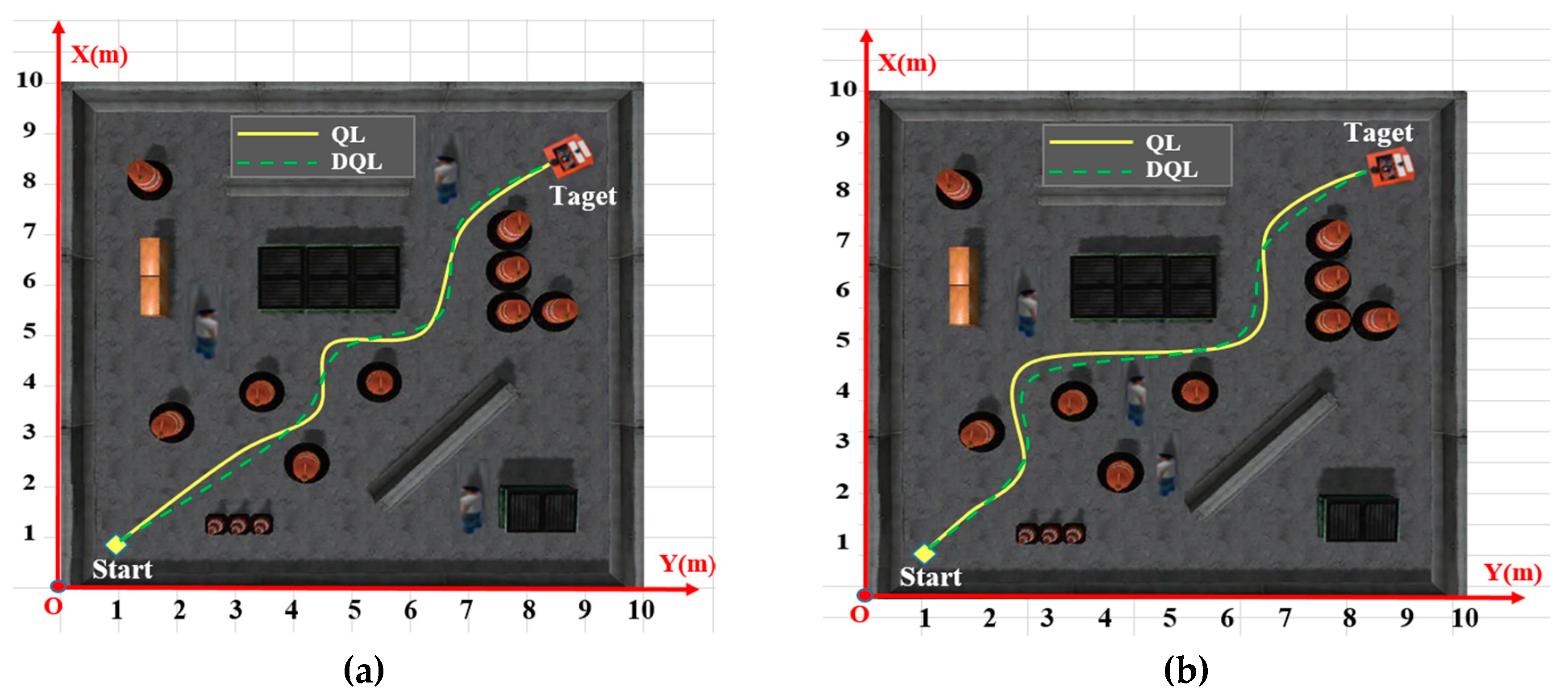
In this environment, various types of obstacles, including pedestrians, static blocks, and walls, were randomly placed to test the performance of the proposed mobile robot navigation algorithm. The task of the robot is to avoid static and dynamic barriers by maintaining a safe distance from them and reaching the target positions in the shortest distance and fastest time. Path planning results of mobile robots using two algorithms, QL and DQL, in dynamic environments.
Figure 9 shows a realistic environment for path planning for a mobile robot, where the workspace is 12m ×12m with obstacles and the minimum distance between blocks is 0.6 m. For all tests, the robot starts from position (1, 1) and finds the path to the target (11, 11). Table 3 below presents the results.
The simulation results in Table 3 show that both controllers ensure the mobile robot plans the optimal path. However, for DQL, the trajectory is improved (shorter distance) but not significantly. Simultaneously, the computation time required to establish the optimal rotation and motion was much better. With the same dynamic environment as the QL algorithm, the course's distance is 16.758m within 12.314s. Still, with the DQL algorithm, the system is 0.429m shorter, but it's almost half the time faster (it takes only 7.927s).

4.6. Experiment Results

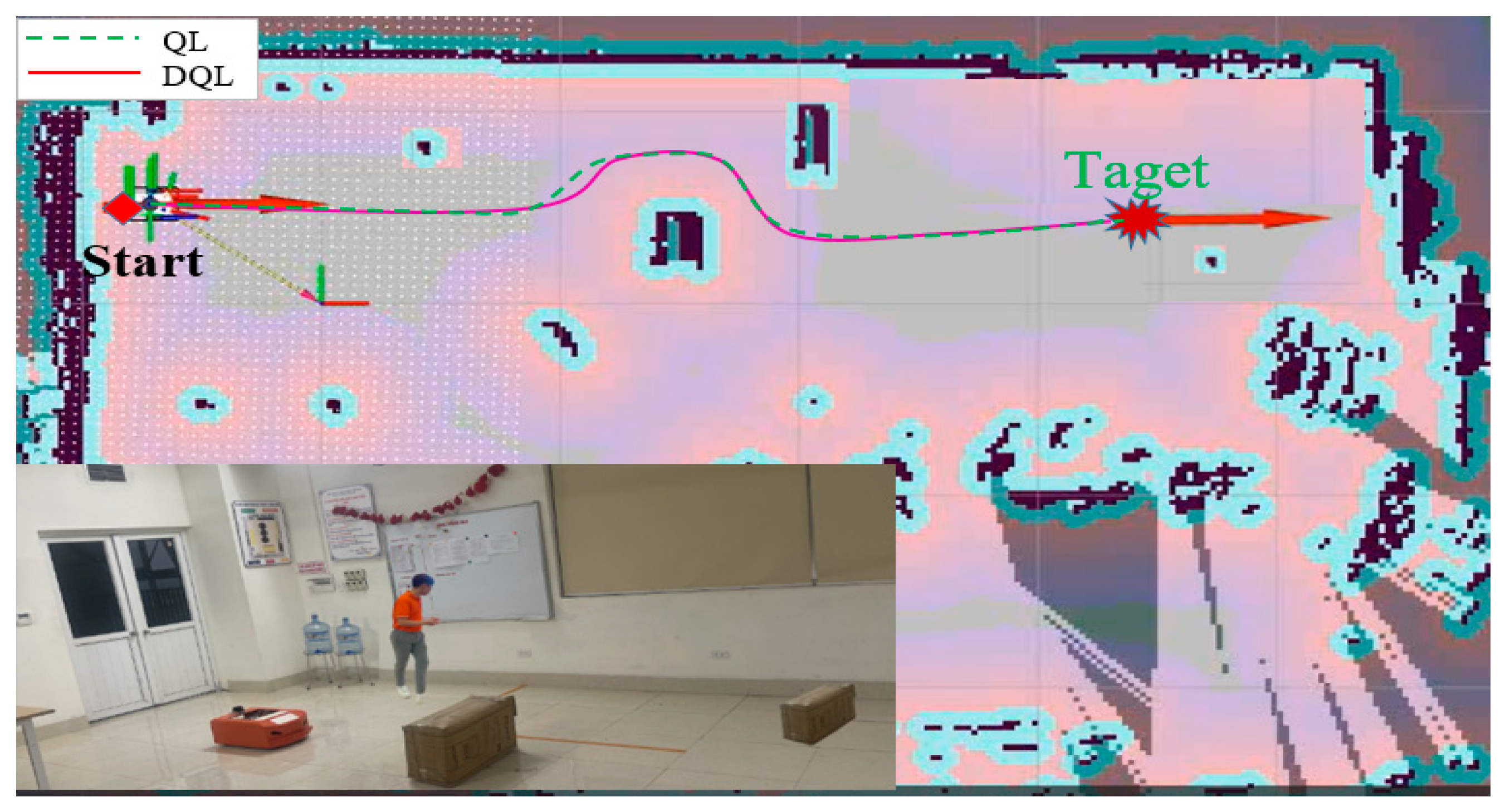
Experimental studies on robots with two proposed algorithms with many obstacles in this environment, including walls, tables, chairs, and students walking. The mobile robot must reach the target while avoiding the static and dynamic barriers (Figure 10). In this study, the robot conducted the following experimental cases:
Case 1: The actual environment for mobile robot path planning, where the workspace is a 4.5m × 6.8m robot club room with obstacles. The experimental study of case 1 is expressed in Figure 11.
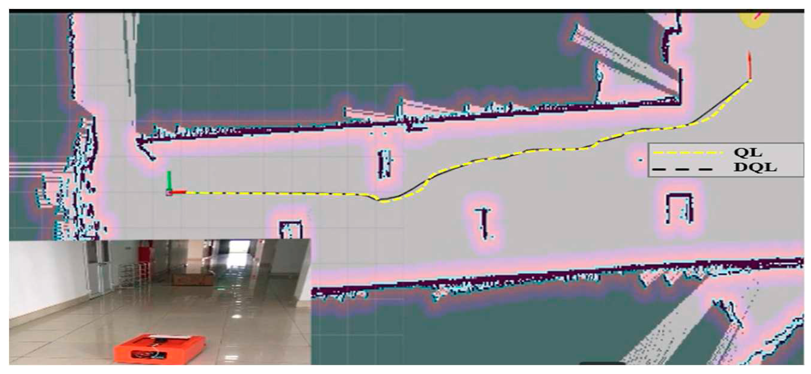
Case 2: A mobile robot running on the hallway. The obstacles in this environment are pillars in the corridor and a cargo box that blocks the middle of the way. The distance from the starting point to the destination in a straight line (bird fly) was 20m. The experimental study of case 2 is expressed in Figure 12.
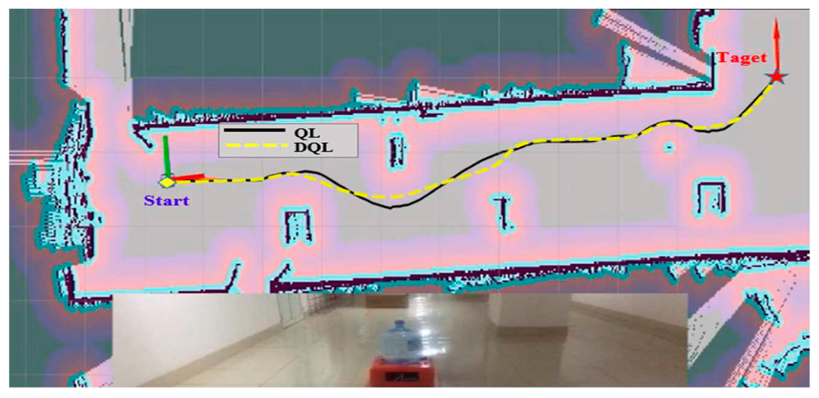
Case 3: The mobile robot runs on the hallway with 20kg, a shown in Figure13. The obstacles in this environment are pillars in the corridor and a cargo box that block the middle of the way. The experimental study of case 3 is expressed in Figure 13.
In Figure 11, Figure 12 and Figure 13 result tests, the mobile robot starts at the door position (1,1) and finds the path to the target (red 5.5m from the door). The experimental results of the two algorithms are listed in Table 4:
Based on the simulation and experimental results, the effectiveness of the DQL algorithm for trajectory planning for mobile robots in an uncertain dynamic environment is demonstrated. The robot establishes an optimal trajectory. In addition, DQL algorithms spend more time in creating high-quality solutions. Furthermore, as the number of barriers increases, so does the execution time variability of the proposed DQL method. By contrast, the DQL technique consistently produces solid results over a short period.
In all three cases, the experimental results show that the results for the DQL algorithm are better than those of the QL algorithm in orbiting planning for mobile robots, particularly in terms of time. In case 1, the orbit for the DQL algorithm was shortened by 0.878 m, and the time is shorter (26.390s) than that of the QL algorithm. Meanwhile, in Case 2, the experiment was the same as in Case 1. The orbit for the DQL algorithm is shortened by 0.88 m, and the time is shorter (26.644s) than that of the QL algorithm. Finally, in Case 3, the orbit for the DQL algorithm was shortened by 1.344m, and the time was shorter (31.279s) than the QL algorithm

5. Conclusions

The Deep Q-Learning (DQL) algorithm is proposed in this study as an optimal path creation solution for mobile robots in complex dynamic environments. The proposed algorithm first helps the robot choose the best action for each situation, then accelerates the learning process for the robot, finds the optimal trajectory, and finally provides the best value of the Q table for each action-state pair in a complex environment. Simulation and experimental results for robots using the DQL algorithm compared with the QL algorithm demonstrated the efficiency and superiority of the proposed algorithm. Therefore, the DQL algorithm should be applied to mobile robots to robot factories combined with computer vision ensure that the trajectory of the mobile robot is accurate and fast.

Author Contributions

All authors contributed equally to this paper. All authors have read and agreed to the published version of the manuscript.

Funding

This research received no external funding.

Data Availability Statement

Not applicable.

Acknowledgments

This project study was supported by all researchers from University Transport and Communications and University of Economics - Technology for Industries.

Conflicts of Interest

The authors declare no conflict of interest

References

  1. Path planning generator for autonomous mobile robots. Robots Auton Syst, 2012, 60: 651–656.
  2. Chaari I, Koubaa A, Trigui S, et al. SmartPATH: an efficient hybrid ACO-GA algorithm for solving the global path planning problem of mobile robots. Int J Adv Robot Syst, 2014, 11: 399-412.
  3. MS Gharajeh and HB Jond, ''An intelligent approach for autonomous mobile robot’s path planning based on adaptive neuro-fuzzy inference system,'' Ain Shams Eng. J. May 2021. [CrossRef]
  4. MS Gharajeh and HB Jond, ''An intelligent approach for autonomous mobile robot’s path planning based on adaptive neuro-fuzzy inference system,'' Ain Shams Eng. J. May 2021. [CrossRef]
  5. C. Zhang, L. C. Zhang, L. Zhou, Y. Li, and Y. Fan, ''A dynamic path planning method for social robots in the home environment,'' Electronics, vol. 9, no. 7, p. 1173, Jul. 2020.
  6. X. Yingqi, S. X. Yingqi, S. Wei, Z. Wen, L. Jingqiao, L. Qinhui, and S. Han, ''A real-time' dynamic path planning method combining artificial potential field method and biased target RRT algorithm,'' J. Phys., Conf. Ser, vol. 1905, no. first, May 2021, Art. no. 012015.
  7. B. Yang, J. B. Yang, J. Yan, Z. Cai, Z. Ding, D. Li, Y. Cao, and L. Guo, ''A novel heuristic emergency path planning method based on vector grid map,'' ISPRS Int. J. Geo-Inf, vol. 10, no. 6, p. 370, May 2021.
  8. S. Xiao, X. S. Xiao, X. Tan, and J. Wang, ''A simulated annealing algorithm and grid map-based UAV coverage path planning method for 3D reconstruction,'' Electronics vol. 10, no. 7, p. 853, Apr. 2021.
  9. T. Lin, ''A path planning method for mobile robot based on A and antcolony algorithms,'' J. Innov. Soc. Sci. Res.vol. 7, no. 1, pp. 157-162, 2020.
  10. Jianming Guo; Liang Liu; Qing Liu; Yongyu Qu, “An Improvement of D* Algorithm for Mobile Robot Path Planning in Partial Unknown Environment” Print ISBN: 978-0-7695-3804-4. [CrossRef]
  11. Lai, X. , Wu, D., Wu, D., Li, JH and Yu, H. (2023), "Enhanced DWA algorithm for local path planning of mobile robot", Industrial Robot, Vol. 50 No. 1, pp. 186 194. [CrossRef]
  12. C. Zong, X. Han, D. Zhang, Y. Liu, W. Zhao, and M. Sun, ''Research on local path planning based on improved RRT algorithm,'' Proc. Inst. Mech. Eng, vol. 235, no. 8, pp. 2086–2100, Mar. 2021.
  13. Tsai, C.C.; Huang, H.C.; Chan, C.K. Parallel elite genetic algorithm and its application to global path planning for autonomous robot navigation. IEEE Trans Ind Electron 2011, 58, 4813–4821. [Google Scholar] [CrossRef]
  14. Saska M, Macaˇs M, Pˇreuˇcil L, et al. Robot path planning using particle swarm optimization of Ferguson splines. Print: Proceedings of IEEE International Conference on Emerging Technologies and Factory Automation (ETFA). New York: IEEE Press, 2006. 833–839.
  15. 9 Raja P, Pugazhenthi S. On-line path planning for mobile robots in dynamic environments. Neural Netw World, 2012, 22: 67–83.
  16. Than Thi Thuong and Vo Thanh Ha, Adaptive Control For Mobile Robots Based On Inteligent Controller, Journal of Applied Science and Engineering, Vol. 27, No 5, Page 2481-2487.
  17. Than Thi Thuong, Vo Thanh Ha, and Le Ngoc Truc, Intelligent Control for Mobile Robots Based on Fuzzy Logic Controller, The International Conference on Intelligent Systems & Networks, ICISN 2023: Intelligent Systems and Networks pp 566–573.
  18. Chen, X.; Kong, Y.; Fang, X.; et al. A fast two-stage ACO algorithm for robotic path planning. Neural Computer Appl 2013, 22, 313–319. [Google Scholar] [CrossRef]
  19. Purcaru, C.; Precup, R.E.; Iercan, D.; et al. Optimal robot path planning using gravitational search algorithm. Int J Artif Intell 2013, 10, 1–20. [Google Scholar]
  20. Li, P.; Duan, H.B. Path planning of unmanned aerial vehicle based on improved gravitational search algorithm. Sci China Technol Sci 2012, 55, 2712–2719. [Google Scholar] [CrossRef]
  21. Duan, H.B.; Qiao, P.X. Pigeon-inspired optimization: a new swarm intelligence optimizer for air robot path planning. Int J Intell Comput Cybern 2014, 7, 24–37. [Google Scholar] [CrossRef]
  22. Liu, J. , Wang, Q., He, C., Jaffrès-Runser, K., Xu, Y., Li, Z., & Xu, Y. (2019). QMR: Q-learning based Multiobjective optimization Routing protocol for Flying Ad Hoc Networks. Computer Communications.
  23. Low, ES, Ong, P., & Cheah, KC (2019). Solving the optimal path planning of a mobile robot using improved Qlearning. Robotics and Autonomous Systems, 115, 143-161.
  24. Luviano, D. , & Yu, W. (2017). Continuous-time path planning for multi-agents with fuzzy reinforcement learning. Journal of Intelligent & Fuzzy Systems, 33(1), 491-501.
  25. Qu, C.; Gai, W.; Zhong, M.; Zhang, J. A novel reinforcement learning based gray wolf optimizer algorithm for unmanned aerial vehicles (UAVs) path planning. Applied Soft Computing 2020, 89, 106099. [Google Scholar] [CrossRef]
  26. Watkins, CJ, & Dayan, P. (1992). Q-learning. Machine learning, 8(3-4), 279-292.
  27. Jaradat, MAK, Al-Rousan, M., & Quadan, L. (2011). Reinforcement based mobile robot navigation in dynamic environment. Robotics and Computer-Integrated Manufacturing, 27(1), 135-149.
  28. Ganapathy, V. , Yun, SC, & Joe, HK (2009, July). Neural Q-learning controller for mobile robot. In 2009 IEEE/ASME International Conference on Advanced Intelligent Mechatronics (pp. 863-868).
  29. Oh, CH, Nakashima, T., & Ishibuchi, H. (1998, May). Initialization of Q-values by fuzzy rules for hastening Qlearning. In 1998 IEEE International Joint Conference on Neural Networks Proceedings. IEEE World Congress on Computational Intelligence (Cat. No. 98CH36227) (Vol. 3, pp. 2051-2056). IEEE.
  30. Jiang, J. , & Xin, J. (2019). Path planning of a mobile robot in a free-space environment using Q-learning. Progress in Artificial Intelligence, 8(1), 133-142.
  31. ] Wang, YH, Li, THS, & Lin, CJ (2013). Backward Q-learning: The combination of Sarsa algorithm and Qlearning. Engineering Applications of Artificial Intelligence, 26(9), 2184-2193.
  32. Das, PK, Mandhata, SC, Behera, HS, & Patro, SN (2012). An improved Q-learning algorithm for pathplanning of a mobile robot. International Journal of Computer Applications, 51(9).
  33. Goswami, I. , Das, PK, Konar, A., & Janarthanan, R. (2010, December). Extended Q-learning algorithm for pathplanning of a mobile robot. In Asia-Pacific Conference on Simulated Evolution and Learning (pp. 379-383). Springer, Berlin, Heidelberg.
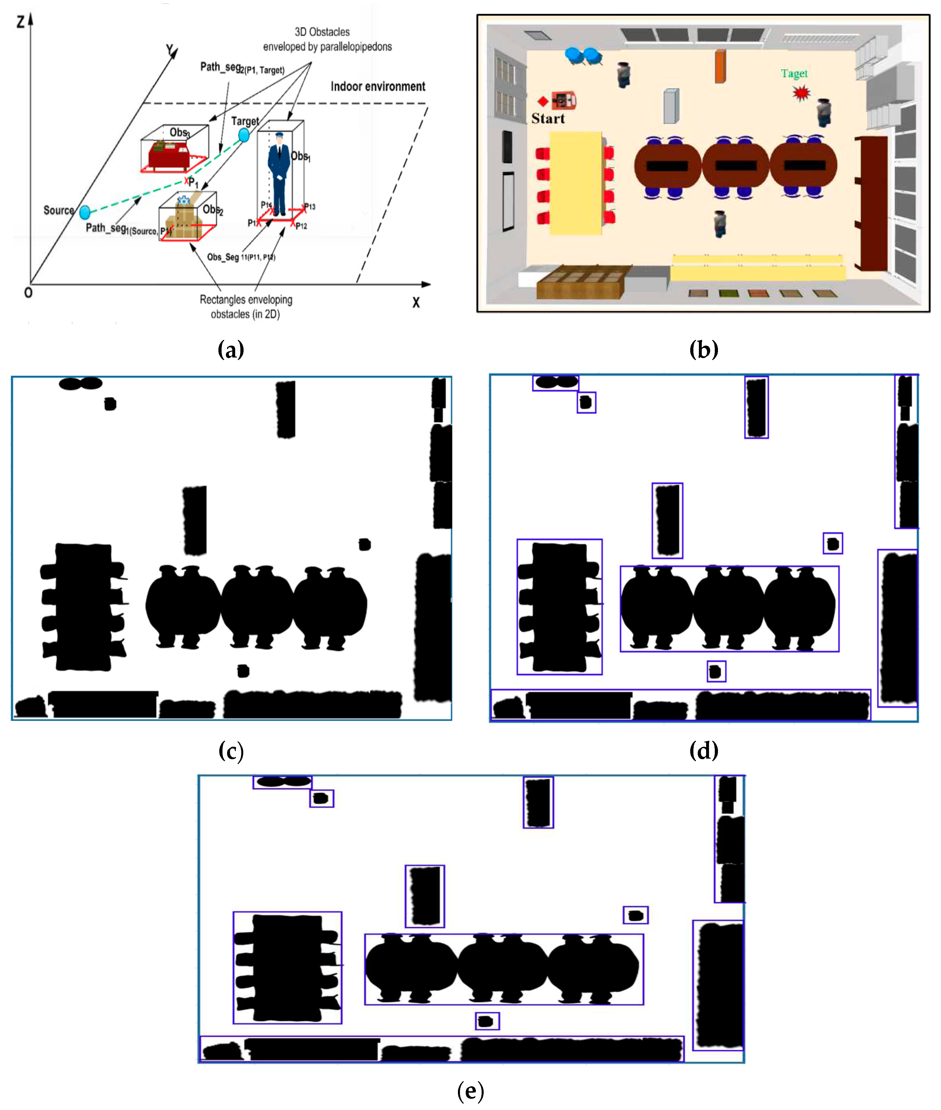
Figure 1. Obstacle estimation for route planning, they should be listed as: (a) Description of 3D modeling of indoor environments; (b) Description of 3D modeling of indoor room; (c) Description of binary map of environment; (d) Description of approximation of the obstacles by rectangles; (e) Description of Binary environment.
Preprints 89856 g001
Figure 2. Q -learning algorithm.
Preprints 89856 g002
Figure 3. The table of Q parameters according to the state-action matrix.
Preprints 89856 g003
Figure 4. Deep Q-learning in Q value assessment.
Preprints 89856 g004
Figure 5. Architectural model.
Preprints 89856 g005
Figure 6. Where 0 is left (-90o), 1 is left front (-45o), 2 is front (0o), 3 is right front (45o), and 4 is right (90o), a mobile robot's actions are directed.
Preprints 89856 g006
Figure 7. Structure diagram of hardware control mobile robot.
Preprints 89856 g007
Figure 8. Path planning simulation environment for mobile robots in ROS-Gazebo.
Preprints 89856 g008
Figure 9. Path planning results of mobile robot using 2 algorithms QL and DQL in dynamic environment, they should be listed as: (a) Case 1; (b) Case 2.
Preprints 89856 g009
Figure 10. Realistic environment of the robot club room.
Preprints 89856 g010
Figure 11. Experimental image of mobile robot movement room.
Preprints 89856 g011
Figure 12. Experiment image of mobile with a robot running in the hallway.
Preprints 89856 g012
Figure 13. Experiment image of mobile with a robot running in the hallway movement room with 20kg.
Preprints 89856 g013
Table 1. Action and Angular.
Action Angular velocity
0 -1.5
1 -0.75
2 0
3 0.75
4 1.5
Table 3. Simulation Results on ROS-GEZABO.
No Algorithm Case 1 Case 2
Distance (m) Run time(s) Distance (m) Run time(s)
1 QL 17.758 12.314 18.416 14.637
2 DQL 17.129 7.927 17.235 8.324
Table 4. Simulation Results on ROS-GEZABO.
No Algorithm Case 1
Distance (m) Run time(s)
1 QL 6.271 72.132
DQL 5.753 47.853
2 QL 6.314 74.097
DQL 5.958 51.845
3 QL 6.264 72.124
DQL 5.386 45.734
Case 2
Distance (m) Run time(s)
1 QL 20.123 57.372
DQL 21.235 32.735
2 QL 20.123 57.375
DQL 21.235 33.738
3 QL 20.123 57.379
DQL 19.235 30.735
Case 3
Distance (m) Run time(s)
1 QL 27.682 92.132
DQL 25.638 87.867
2 QL 27.682 92.132
DQL 25.638 87.656
3 QL 27.682 92.132
DQL 26.338 60.853
Disclaimer/Publisher’s Note: The statements, opinions and data contained in all publications are solely those of the individual author(s) and contributor(s) and not of MDPI and/or the editor(s). MDPI and/or the editor(s) disclaim responsibility for any injury to people or property resulting from any ideas, methods, instructions or products referred to in the content.
Copyright: This open access article is published under a Creative Commons CC BY 4.0 license, which permit the free download, distribution, and reuse, provided that the author and preprint are cited in any reuse.
Prerpints.org logo

Preprints.org is a free preprint server supported by MDPI in Basel, Switzerland.

Subscribe

© 2024 MDPI (Basel, Switzerland) unless otherwise stated