Using Linear Regression to Reduce Measurement Errors for Electric Power

Preprint

Article

Using Linear Regression to Reduce Measurement Errors for Electric Power

Altmetrics

Downloads

Views

Comments

Constantin-Daniel Oancea^*

This version is not peer-reviewed

Submitted:

06 November 2023

Posted:

07 November 2023

You are already at the latest version

Alerts

Abstract

Although data acquisition is a very usual technique, there are several aspects not always considered, as synchronization of acquired measures and evaluation of the errors that derive from this fact. The paper hereby aims to point this thing out, by mathematical determination of the necessary correction and implementing the software meant to evaluate the performances of the acquisition system. As an example, a three-phased acquisition system has been developed in order to monitor the currents and voltages on the three phases. Also other measures have been calculated, such as power and phase. The components on each phase don’t have to be fully identified because a whole system calibration can be made in the first stage. Calibration consists in finding the weighting coefficients for each quantity. The implemented solution for three-phased measures data acquisition starts from the hypothesis of a sampling frequency that respects Shannon theorem. The distance between two samples is small enough to consider a linear evolution between two moments for the same measure. Errors that affect the above mentioned, due to the different moments of time when samples are acquired, are analyzed and brought to the minimum value.

Keywords:

Subject: Engineering - Electrical and Electronic Engineering

1. Introduction

Critical real-time data acquisition and control is an important issue in data acquisition systems. Applications that require real-time control are better suited to external systems than to systems based on plug-in PC boards. For example and tests, a horse system with MS windows operating system and an older model computer was used, on which the subject of this article can be more easily followed. Although Microsoft Windows has become the standard operating system for PC applications, it is an indeterminate operating system in terms of time response in measurement and control applications, [1].

A "plug-in" board and the LabVIEW programming environment are used for the experiment. LabVIEW stands out from the usual programming languages through the features of a graphical programming language environment ("G" programming), with all the necessary tools for data acquisition, signal analysis and their presentation. The board used, AT-MIO-16, is a National Instruments manufacturing board (1992), hardware configurable, but also software, which has as main characteristics 16 analog inputs, two 12-bit CDAs with voltage outputs, 8 lines TTL-compatible digital signal I/O and 3 16-bit counter/clock channels, being provided with RTSI bus (Real-Time System Integration), a system that allows the synchronization of multiple measurements made by means of other AT-type acquisition boards linked on the same highway. This board was chosen to highlight the errors that affect the process of converting analog quantities and using them to determine other quantities, [2].

2. Materials and Methods

Like video adapters, modems, and other types of expansion cards, plug-in data acquisition cards are designed to fit into computer motherboard slots, being connected directly to computer buses. Viewed as a category, plug-in boards offer a wealth of test functions, a high number of channels, high speed, and adequate sensitivity to measure low-level signals, at a relatively low cost.

The implementation of a data acquisition system was originally a self-powered system that exchanged information with a computer through a standard interface. As an in-house alternative to plug-in boards, this type of system usually offers more I/O channels, a quieter electrical environment, greater flexibility and speed adapted to different applications.

For a system in which high performance is required and its purchase price and installation will increase, but for the measurement system presented, both the acquisition board used and the operating system in which it was integrated are suitable for the needs, at a modest price. The choice of the acquisition board first of all involves the choice of the sampling speed of the analog-to-digital converter, which is mainly the one that dictates the price of the acquisition board. Although the board used does not have a high sampling rate, it being only 100 [kS/s], this is sufficient to carry out the experiment in compliance with Shannon's theorem, remembering the frequency of the network is 50 [Hz] in Europe. Thus, the distance between two successive samples is small enough to be able to consider a practically linear evolution between two successive moments of the same size. The experimental results indicate little difference between the direct and corrected results. The importance of this correction appears at high powers or when using a sampling frequency lowers than a minimum of 10-20 times the maximum frequency desired to be taken into account, [3].

Due to the different moments of time, on each channel, in which the acquisition takes place, the determination of the active power, as an average of the instantaneous power, can be affected by errors. Thus, the multiplication of the voltage vector with the current vector, although it is done at the same index, however in reality they are at different moments of time, offset by a sampling step.

2.1. Echipment Design

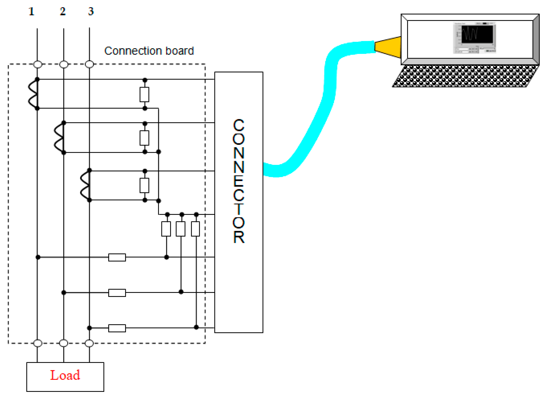
The measuring circuit is made up of a series of specific elements, which allow comparisons but also the avoidance of a dangerous regime for the acquisition board, but also specific elements such as the adaptation-attenuation circuits that bring the voltage and current from the network to a level acceptable to the acquisition board, Figure 1.

The currents are transformed into acceptable voltages by the board by means of current transformers and resistors connected in the secondary. To adapt the voltage levels, resistive dividers were provided. They provide an unaltered waveform, without additional phase shift, but have the disadvantage that they do not provide galvanic isolation of the acquisition board from the three-phase network. Rigorous identity between the components on each phase is not required, as a software calibration of the entire assembly can be performed in a first phase. Calibration consists in finding weighting coefficients for each size, so that the displayed value corresponds to the measured value, [4].

2.2. The Measurement, Processing and Display Application

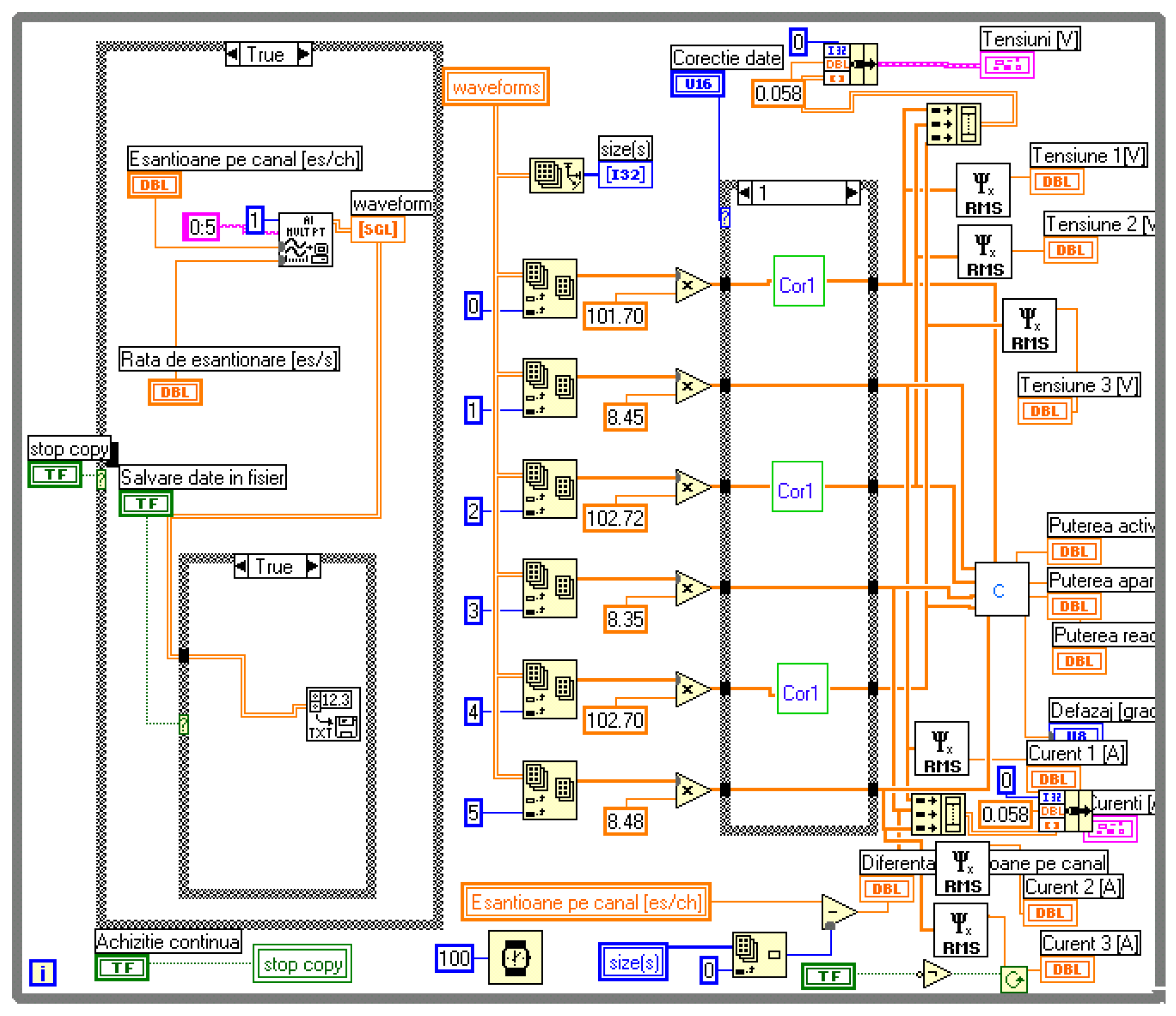
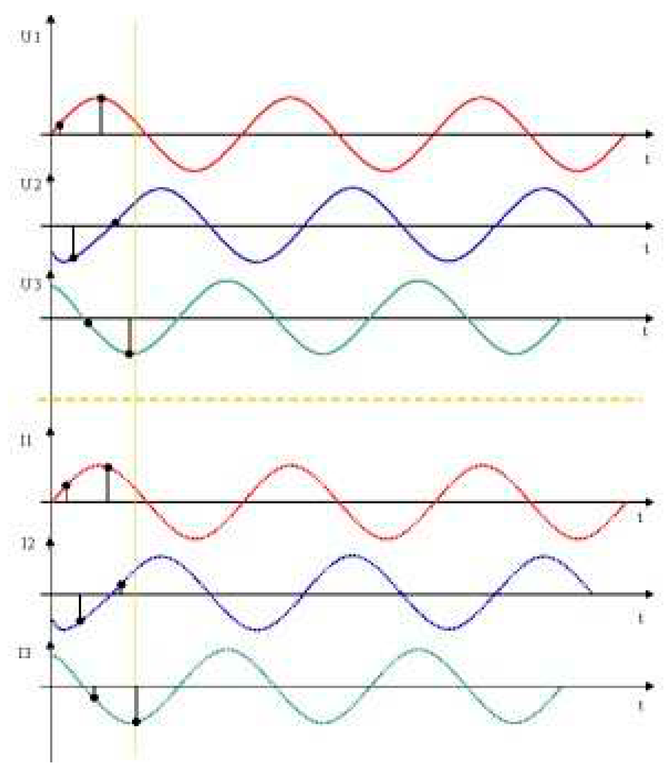
For the application, the connection diagram made is shown in Figure 2. The signals received by the acquisition board are 3 voltages (u1, u2, u3) and 3 currents (i1, i2, i3), in the form shown in Figure 3. The data sequence that is repeated is u1, i1, u2, i2, u3, i3. When imposing the frequency of samples and the number of samples, it must be taken into account that they must be a multiple of 6, for taking a whole number of samples, the same for each size. Due to the different moments of time, Figure 3, on each channel, in which the acquisition takes place, the determination of the active power, as an average of the instantaneous power, can be affected by errors. In order to determine several quantities, it is necessary to carry out some mathematical operations between them. Some powers, phase shifts, different coefficients are determined by mathematical operations. Even if mathematically it is simple to operate, there is the possibility of an impediment of the nature of physical phenomena, [5].

In order to make the necessary correction, it is proposed to use some mathematical evaluations, to determine the value corresponding to the moment of time considered. From Figure 3 it can be seen that between u1 and i1 there is a gap of one sampling step, but the next value is found over 5 sampling steps.

2.3. Algorithm Proposed

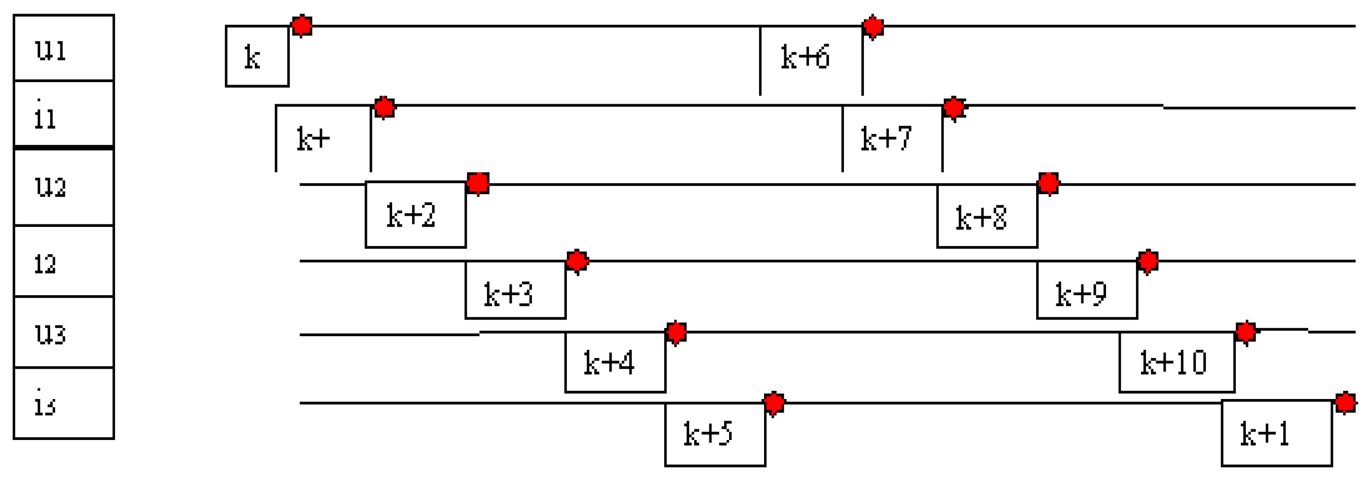
Due to the different moments of time, Figure 3, on each channel, in which the acquisition takes place, the determination of the active power, as an average of the instantaneous power, can be affected by errors. Thus, the multiplication of the voltage vector with the current vector, although it is done at the same index, however in reality they are at different moments of time, offset by a sampling step. Figure 4 summarizes this sequence.

In order to make the necessary correction, it is proposed to use some mathematical evaluations, to determine the value corresponding to the moment of time considered. From Figure 4 it can be seen that between u1 and i1 there is a gap of one sampling step, but the next value is found over 5 sampling steps.

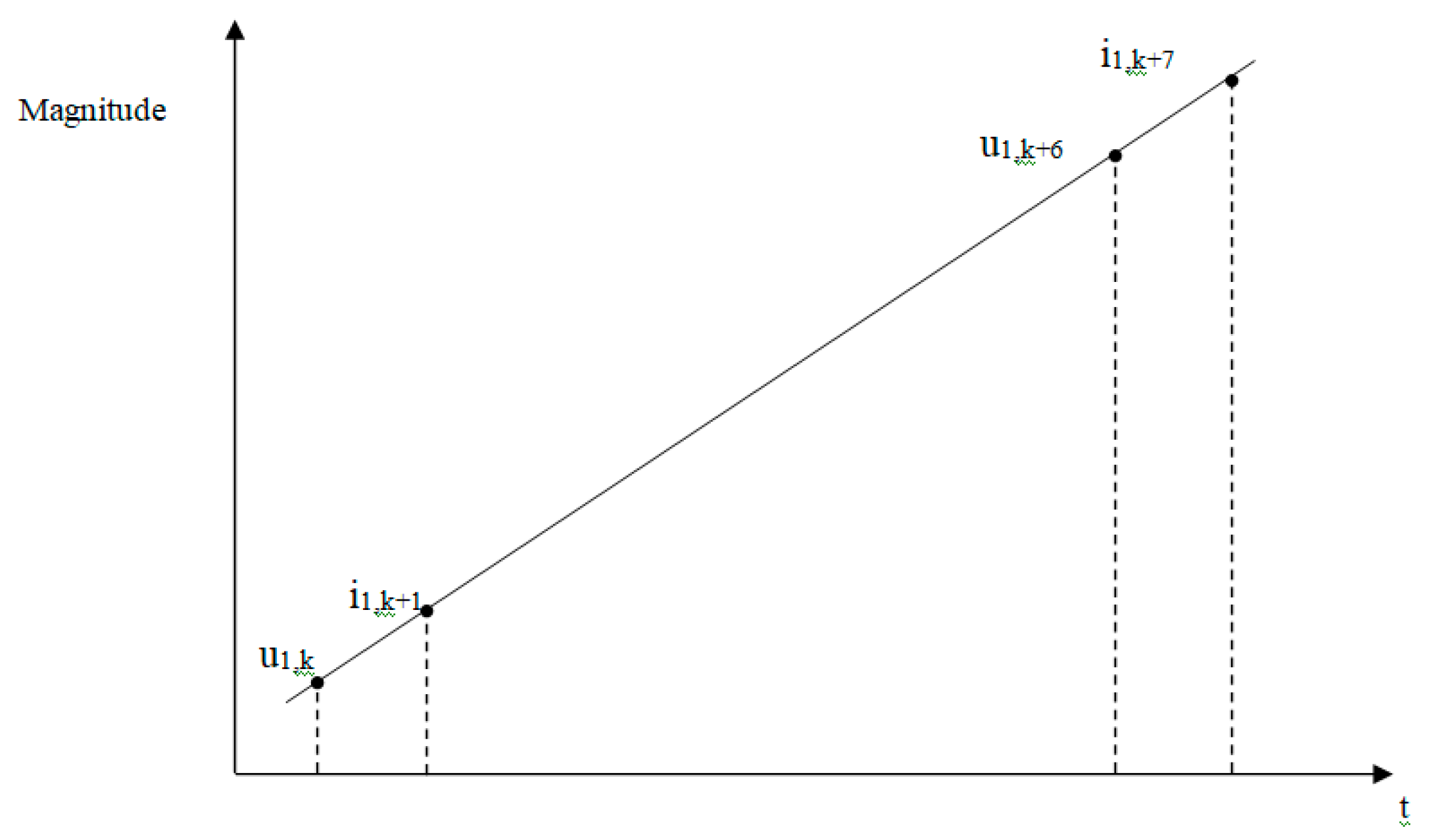
To determine the equations, Figure 5 presents the methodology for calculating the intermediate values (a linear variation is approximated over the considered interval). Can be use any expression of function (polynomial, logarithmic, etc.), but because of small distance between samples and easily calculation, was choose linear approximation, [6,7,8].

Considering that the signal variations are linear between two successive moments, it is proposed as a solution for determining the values at the same moment of time, interpolation/extrapolation to find the intermediate values, with the necessary changes at the ends of the acquired values vector.

We can do the correction even on voltages or currents. The following relation presents mathematical approaches.

Voltage correction equations is (1)-(5), with variants for interpolation and extrapolation, (6)-(8) respectively (9)-(11). A and B are constants and t_k is moment of time at step k.

u_{k} = A \cdot t_{k} + B

(1)

u_{k + 6} = A \cdot t_{k + 6} + B

(2)

u_{k} - u_{k + 6} = A \cdot (t_{k} - t_{k + 6}) = (- 6) \cdot A \cdot t

(3)

A = \frac{u_{k + 6} - u_{k}}{6 \cdot t}

(4)

B = u_{k} - A \cdot t_{k} = u_{k} - \frac{u_{k + 6} - u_{k}}{6 \cdot t} \cdot t_{k} = u_{k} + \frac{u_{k} - u_{k + 6}}{6 \cdot t} \cdot t_{k}

(5)

u_{k + 1} = A \cdot t_{k + 1} + B

(6)

u_{k + 1} = \frac{u_{k + 6} - u_{k}}{6 \cdot t} \cdot t_{k + 1} + u_{k} + \frac{u_{k} - u_{k + 6}}{6 \cdot t} \cdot t_{k}

(7)

u_{k + 1} = \frac{5 \cdot u_{k} + u_{k + 6}}{6}

(8)

u_{k + 7} = A \cdot t_{k + 7} + B

(9)

u_{k + 7} = \frac{u_{k + 6} - u_{k}}{6 \cdot t} \cdot t_{k + 7} + u_{k} + \frac{u_{k} - u_{k + 6}}{6 \cdot t} \cdot t_{k}

(10)

u_{k + 7} = \frac{- u_{k} + 7 \cdot u_{k + 6}}{6}

(11)

The order of the samples being u1k, i1k, u2k, i2k, u3k, i3k, if the correction is made for the voltage values, the first n/6-1 values will be corrected by interpolation, and the last value will be determined by extrapolation. If the current correction is considered, the first value is calculated by extrapolation and the rest by interpolation.

Since extrapolation involves a less predictable evaluation of the values, it is recommended to use interpolation to determine the required values.

3. Results

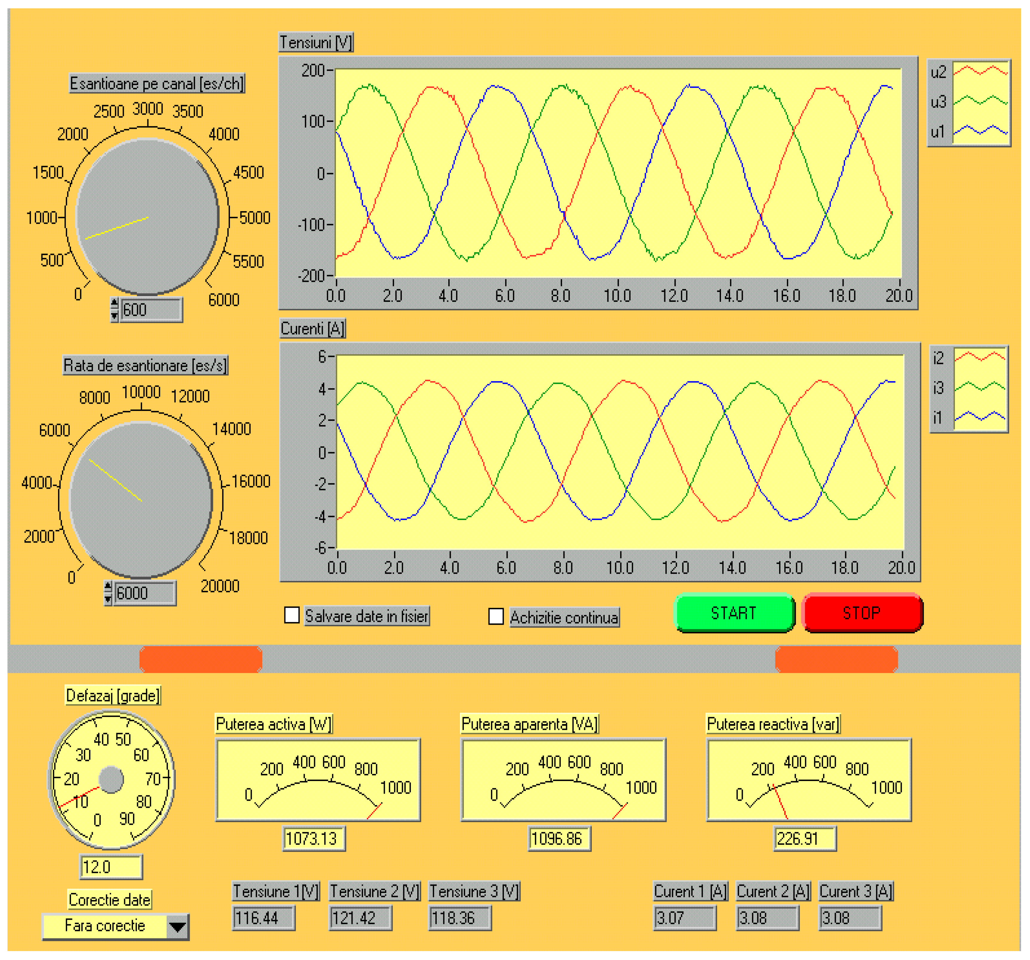
The front panel of the application is presented in Figure 6, representing the voltage correction situation, [9,10,11]. Even if the difference from the value of the active power for the situation without correction is around 1 W, on a large scale this component adds up, becoming significant.

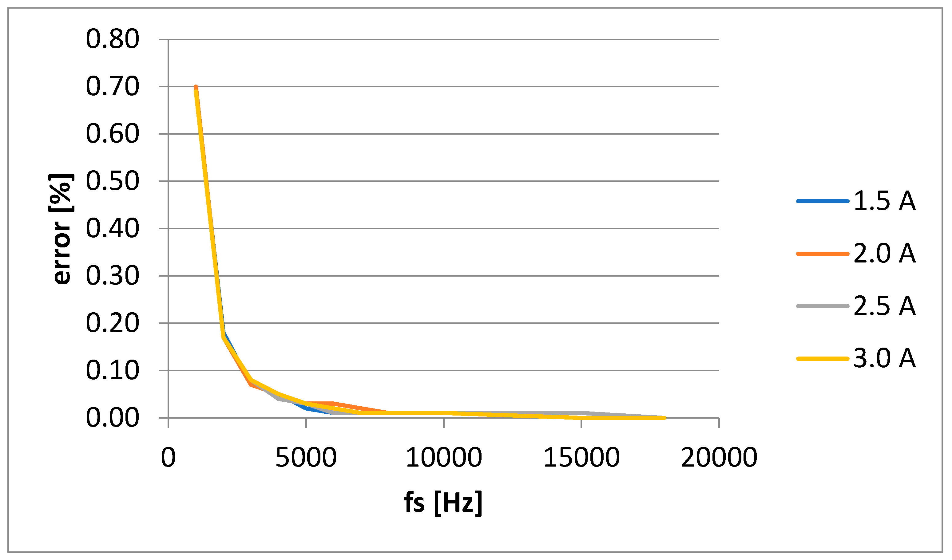
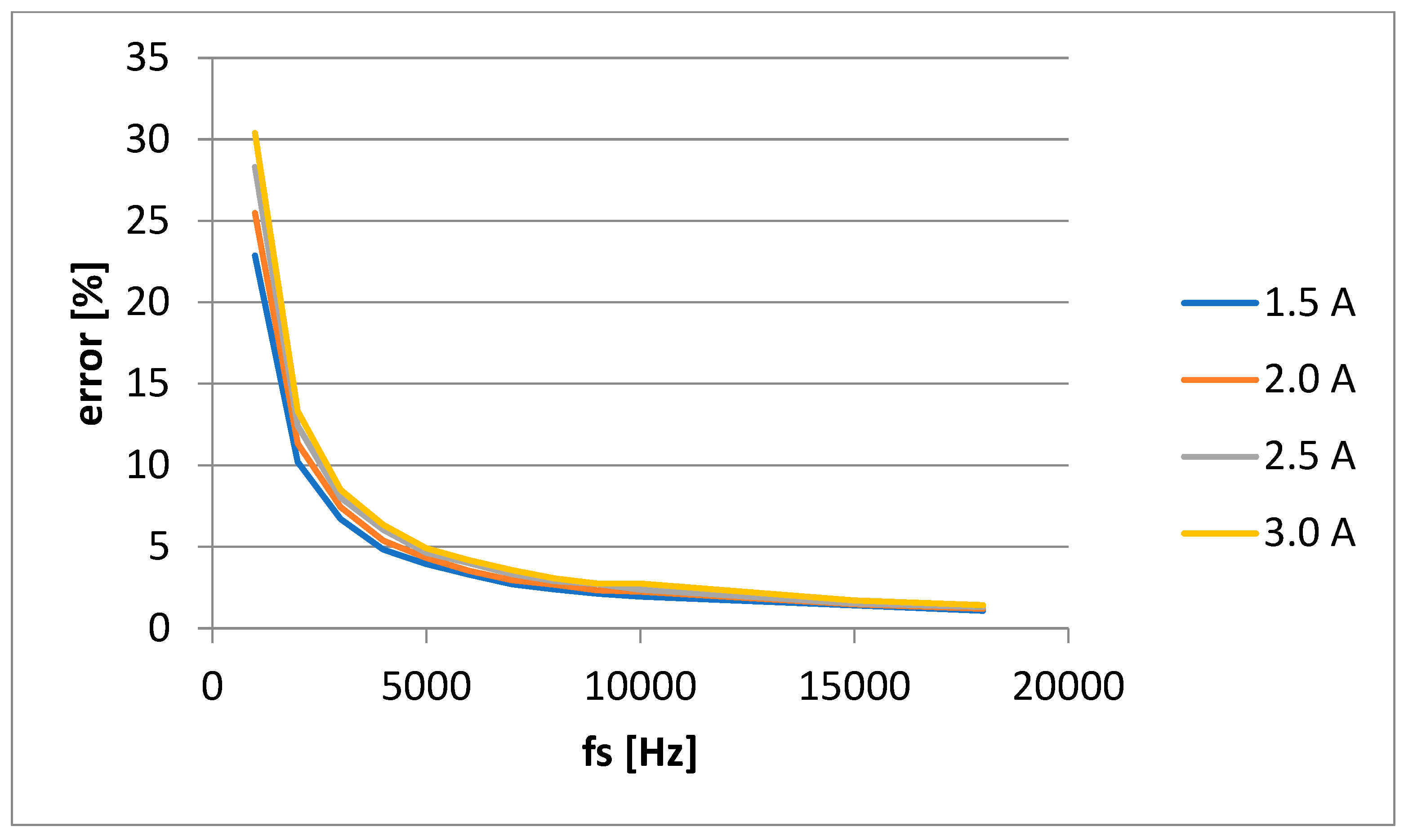
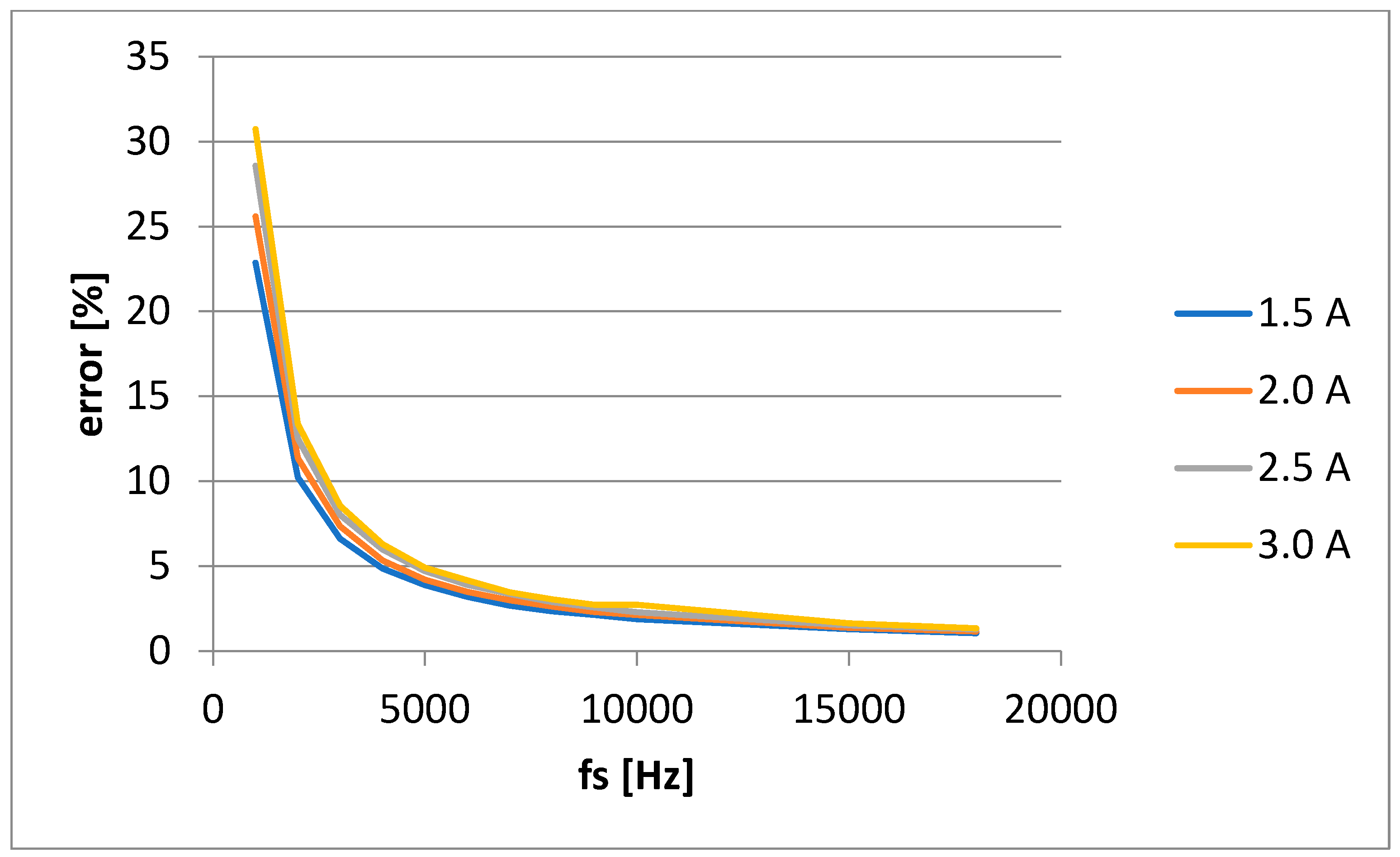
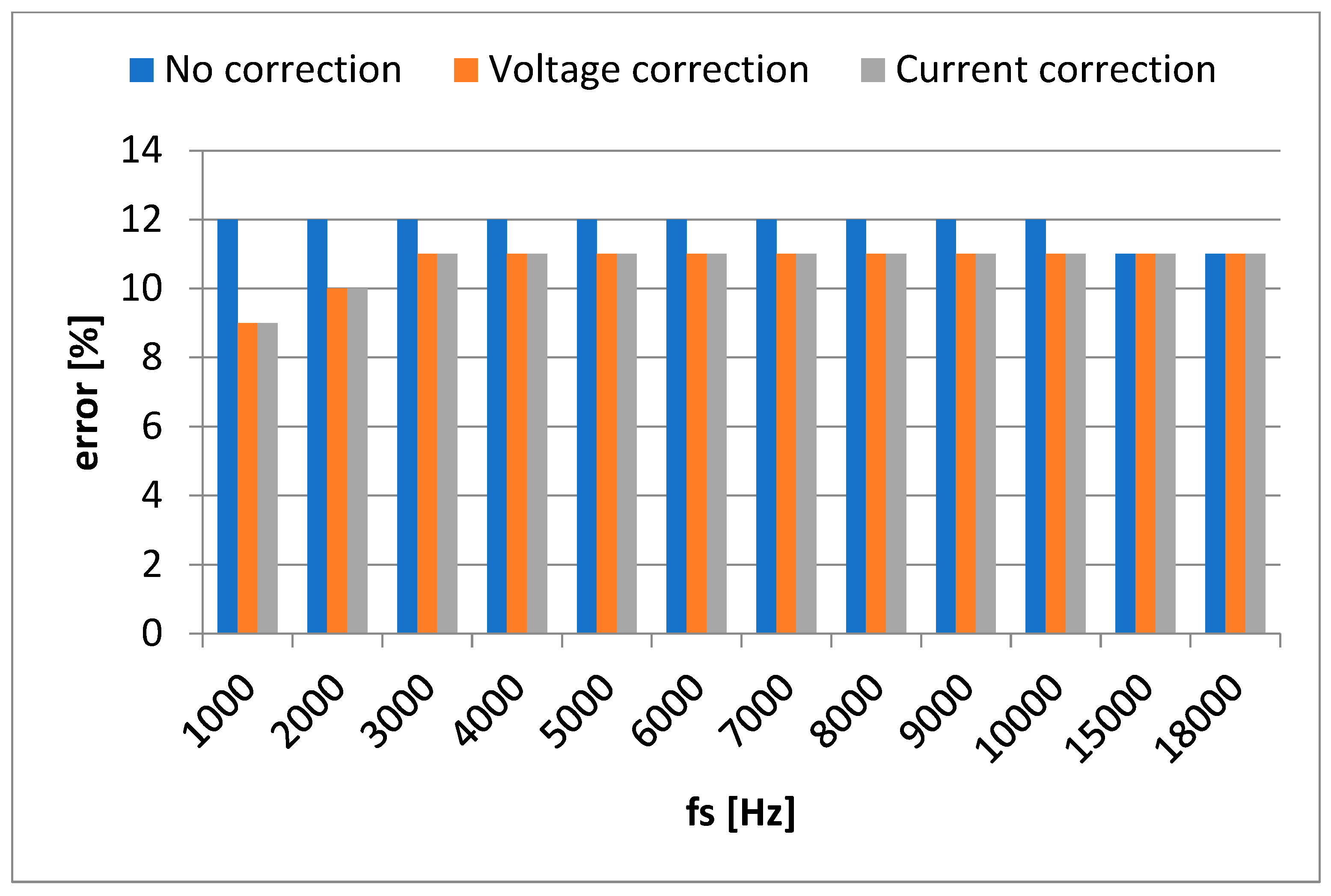
The experimental results are for different sampling frequencies, which affects the results. The reported errors were calculated by relating the uncorrected values to the corrected ones. The quantities for which they were calculated are: sampling frequency, active power, apparent power and reactive power. The measurements were made for different loads of 1.5, 2, 2.5 and 3 amperes.

The load used is of the R-L type (resistance-inductance), there is a inductive phase shift in the circuit of approximately 11-12 degrees.

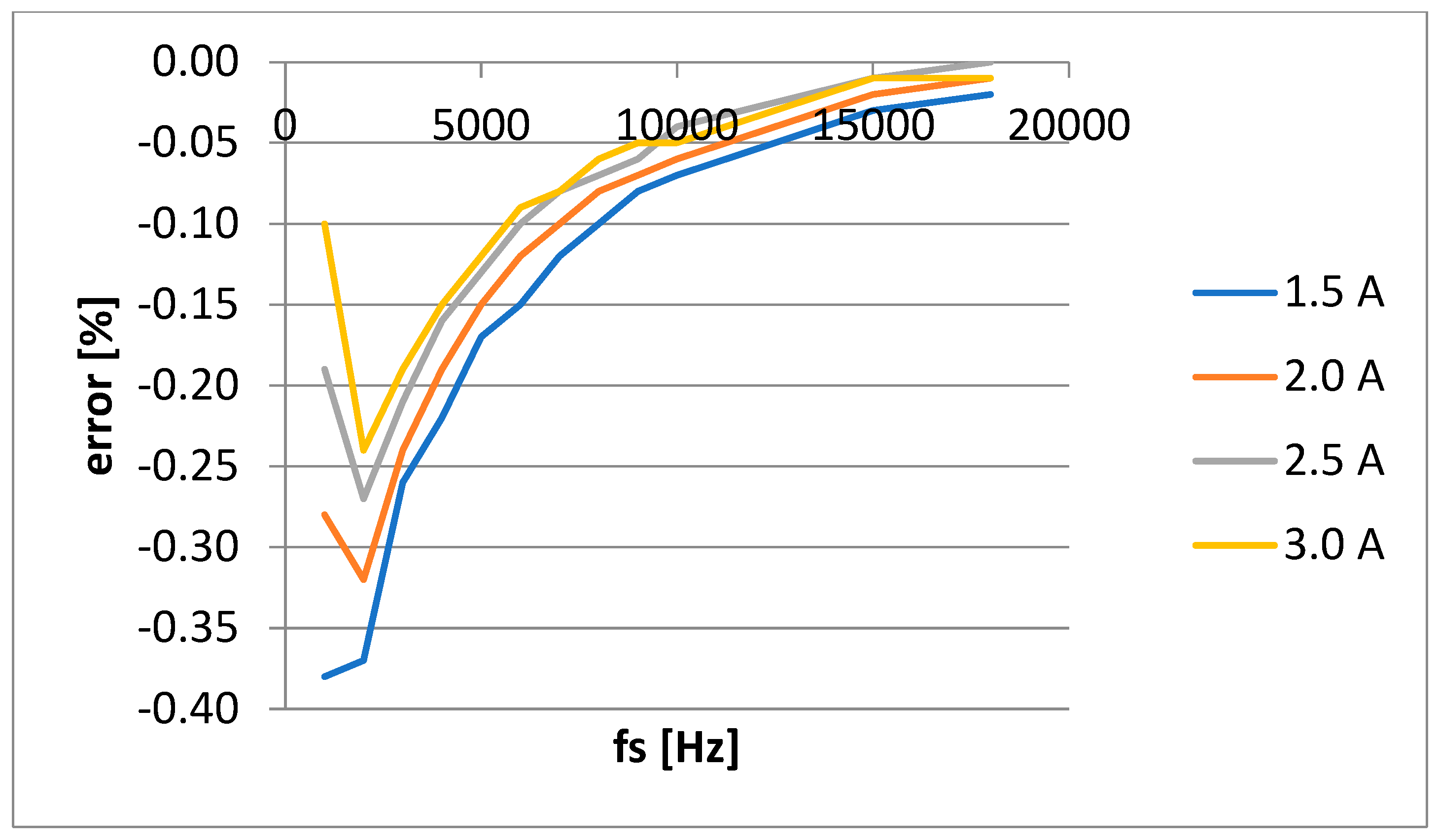
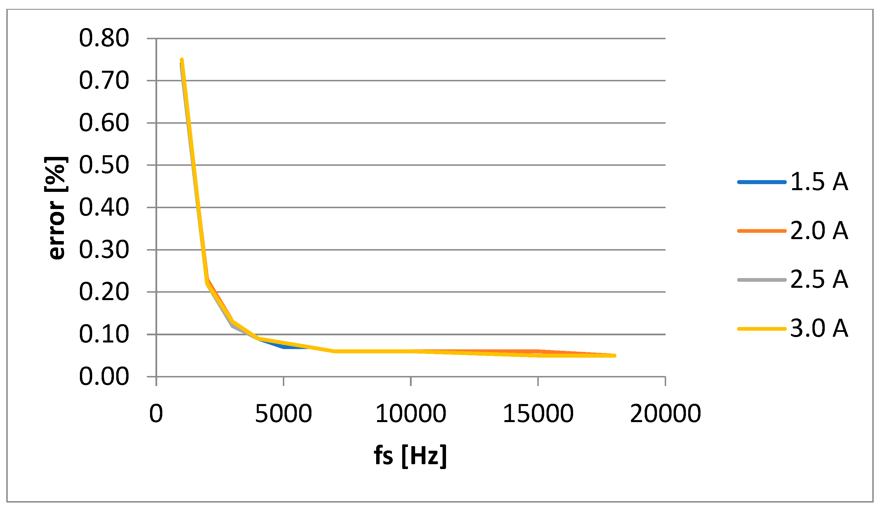
Figure 7 and Figure 8 show the case of errors (vs. sampling frequency, fs [Hz]) affecting the active power measurement.

The small error differences in the case of active power (P) are due to the use of an appropriate sampling frequency. But even the sampling frequency is adequate, sampling error still exist. It can be observed that there is a special behavior in the area of low sampling frequencies for the active power. An explanation would be inductive component of load which imposes a reactive component with large errors at low sampling frequency.

Apparent power, S, have a different shape, for all loads (1.5, 2, 2.5 and 3 A), having the same behavior. For the apparent power, the errors are practically the same because the RMS values are the same, theoretically, regardless of the sampling frequency. The differences that appear between the values with or without correction are due to changes in the amplitude of the signals due to the applied interpolation/extrapolation. The error is increasing significantly to lower sampling frequency, Figure 9 and Figure 10. Without using this correction, errors became significant in some conditions.

The errors increase with the decrease of the current, because at low currents, non-linearity errors of the measuring chain components also appear.

We must remember that the acquisition board was chosen with low performance just to highlight this error. It is obvious that for acquisition boards with higher performance (higher sampling frequency or lower number of channels), sampling error has lower values.

The last power analyzed is reactive power, Q, of the same load (resistive-inductive), Figure 11 and Figure 12. Because of load used, about small reactive component, around 10 degree shift phase, the error is much more than previously electric power types (active and apparent).

If the load had a strong reactive character, the errors would have been inversely proportional, for active power it would have been higher and for reactive power lower.

Another important problem is that if the board does not have a correlation between the number of points acquired and the sampling frequency, the first value having fixed intrinsic values, and the second being continuously variable between 300 and 18000Hz. If a certain ratio, constant between the two sizes, is not respected, this can be another source of additional errors.

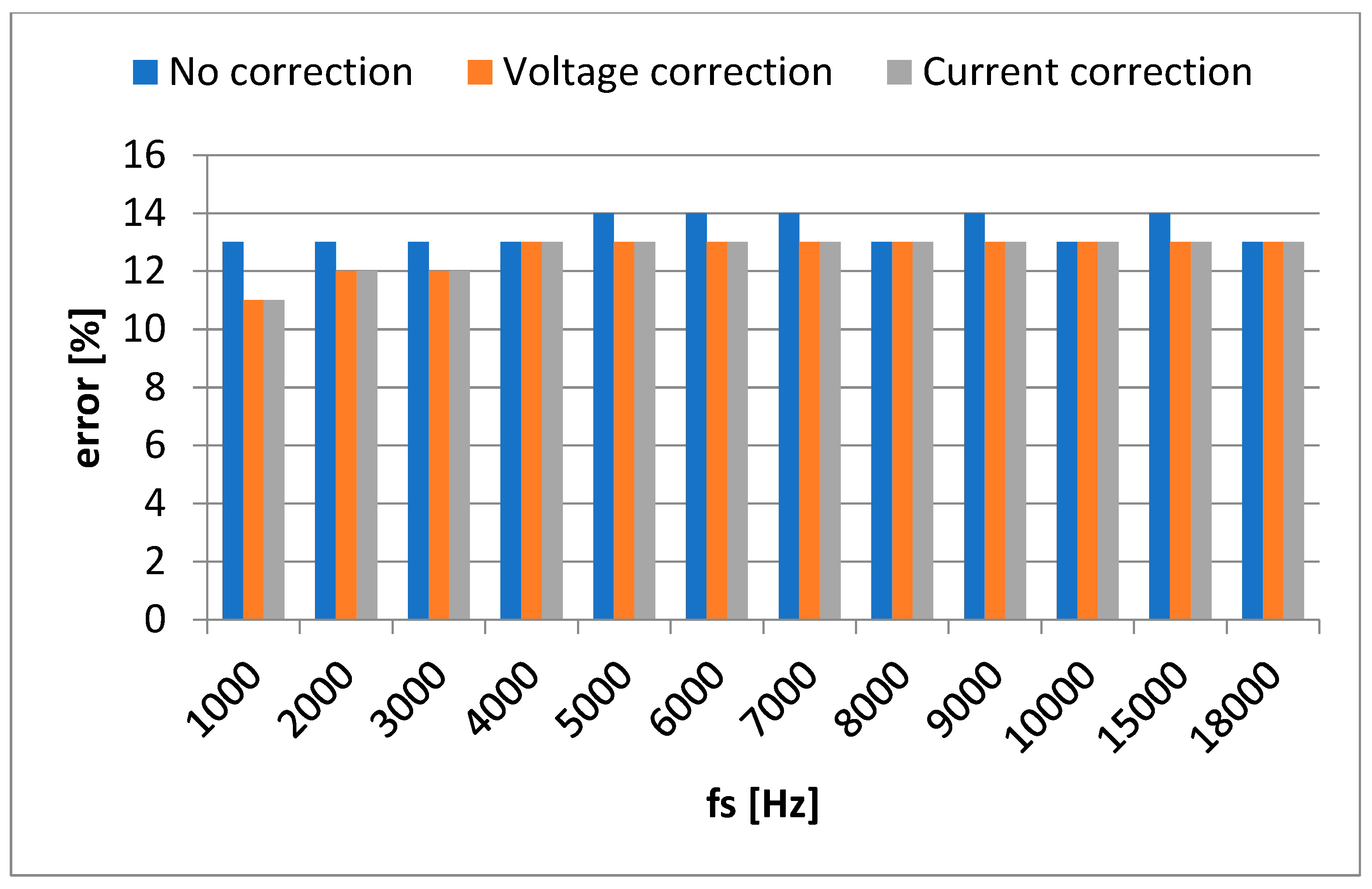
An aspect to point out is the differentiation of the phase shift values, depending on the sampling frequency and the load. The “arcos” trigonometric function applied to the P/S ratio was used for the determination. The “arcsine” formula could also be used on the Q/S ratio, but the errors accumulate, the result being affected by larger errors than in the first situation. It is remarkable that after a certain sampling frequency, 4000Hz, the corrected results for voltage and current correction are overlaping, Figure 13 (2 A load) and Figure 14 (3 A load).

A remark is that the results are affected by the load, changing the slope at each point on the current.

4. Discussion

The architecture for data acquisition and control is available in a number of forms, which offer various possibilities of operation, number of channels, speed, resolution, accuracy and cost.

Plug-in data acquisition boards are an important category. Like display adapters, modems, and other types of expansion cards, plug-in data acquisition cards are designed to fit into computer motherboard slots.

Viewed as a category, plug-in boards offer a wealth of test functions, a high number of channels, high speed, and adequate sensitivity to measure low-level signals, at a relatively low cost.

External data acquisition systems represent another category within data acquisition systems.

For economic reasons, a common "plug-in" acquisition board was chosen in the work. The first step in the design of such a system is the choice of the acquisition board, depending on its performance and its use. Since the quantities to be measured are known, an optimal purchase plate will be chosen. For a system in which high performance is required and its purchase price and installation will increase, but for the measurement system presented, both the acquisition board used and the operating system in which it was integrated are suitable for the needs, at a modest price. The choice of the acquisition board first of all involves the compatibility of the sampling speed of the analog-to-digital converter, which is mainly the one that dictates the price of the acquisition board. Although the board used does not have a high sampling rate, being only 100 [kS/s], this is sufficient for the chosen utility, where the network frequency is 50 [Hz]. The maximum order of harmonics that can be visualized is 30-40, respecting Shannon's theorem. Another problem is the number of input channels available, and their reference mode. The chosen board has 16 input channels for analog signals with a reference, much more than the required 6 channels + a ground, used in this work.

The solution implemented for data acquisition of some quantities from the three-phase system, starts from the assumption of a sampling frequency that respects Shanon's theorem, being sufficiently high. Thus, the distance between two successive samples is small enough to be able to consider a practically linear evolution between two successive moments of the same size. The experimental results indicate little difference between the direct and corrected results. The importance of this correction appears at high powers or when using a sampling frequency lowers than a minimum of 10-20 times the maximum frequency desired to be taken into account.

To make the necessary correction, the mathematical evaluation is used to determine the value corresponding to the moment of time considered. Considering that the signal variations are linear between two successive moments, interpolation/extrapolation to find the intermediate values is proposed as a solution for determining the values at the same moment of time, with the modification.

It is observed, in case of active power, Figure 7 and Figure 8, which the errors increase with the decrease of the sampling frequency. It is also found that the errors for current correction are larger, due to the fact that the first calculated value is obtained by extrapolation, the series of subsequent values being dependent on it. So it is recommended to go, initially, to determine the values by interpolation and not by extrapolation. If it had started with the first value, the current, then the current correction method would have been the one indicated. The errors increase with the decrease of the current, because at low currents, non-linearity errors of the measuring chain components also appear. The differences that appear between the values with or without correction are due to changes in the amplitude of the signals due to the applied interpolation/extrapolation.

5. Conclusions

The article presents a software method by which, using low-cost data acquisition boards, superior performance can be obtained regarding the accuracy of measurements, in systems that require the measurement of several quantities and the determination of others based on them. For example, by acquiring a voltage and a current, the power is calculated (active, apparent, and reactive, as the case may be). If it were not taken into account that the reading of the data is not done at the same time for the two quantities, the result is not correct. The proposed method is very efficient, the approximation used being applicable, especially for high sampling frequencies, when a linear variation of the input quantities (voltage, current) can be approximated.

Funding

This research received no external funding.

Institutional Review Board Statement

Not applicable

Informed Consent Statement

Not applicable.

Conflicts of Interest

The authors declare no conflict of interest.

References

Lin, A.Y.; Arabandi, S.; Beale, T.; Duncan, W.D.; Hicks, A.; Hogan, W.R.; Jensen, M.; Koppel, R.; Martínez-Costa, C.; Nytrø, Ø.; et al. Improving the Quality and Utility of Electronic Health Record Data through Ontologies. Standards 2023, 3, 316-340. [CrossRef]
Kuppusamy, R.; Nikolovski, S.; Teekaraman, Y. Review of Machine Learning Techniques for Power Quality Performance Evaluation in Grid-Connected Systems. Sustainability 2023, 15, 15055. [CrossRef]
*** Data Acquisition and Control Handbook, 1st Edition, Keithley, Printed in U.S.A., 2001.
Niţă, L., Creţu, M., Foşalău, C., Postolache, O., Computer interfacing and programming for the realization of IT measurement systems, MatrixRom Publishing House, Bucharest, 2000.
Oancea, C.D., Oancea, C., Computer aided measurements, Printech Publishing House, Bucharest,2002.
*** — Handbook. Application to solution, Quatech, 1999.
Abdel-Fattah, M.K.; Kotb Abd-Elmabod, S.; Zhang, Z.; Merwad, A.-R.M.A. Exploring the Applicability of Regression Models and Artificial Neural Networks for Calculating Reference Evapotranspiration in Arid Regions. Sustainability 2023, 15, 15494. [CrossRef]
Casesnoves, F. Genetic Algorithms for Interior Comparative Optimization of Standard BCS Parameters in Selected Superconductors and High-Temperature Superconductors. Standards 2022, 2, 430-448. [CrossRef]
*** LabVIEW Development Guidelines; April 2003 Edition; National Instruments Corp. Austin, Texas, U.S.A.
*** LabVIEW User Manual; April 2003 Edition; National Instruments Corp. Austin, Texas, U.S.A.
www.ni.com, last accesed October 3^rd 2023.

Figure 1. Sketch for error analysis in a three-phase quantity acquisition system.

Figure 2. Partial block diagram (with calibration coefficients) associated with the front panel.

Figure 3. Evolution of signals and samples.

Figure 4. The sequence of samples.

Figure 5. Explanatory figure for the calculation of intermediate values.

Figure 6. Front panel of application.

Figure 7. Active power measurement error, voltage correction.

Figure 8. Active power measurement error, current correction.

Figure 9. Apparent power measurement error, voltage correction.

Figure 10. Apparent power measurement error, current correction.

Figure 11. Reactive power measurement error, voltage correction.

Figure 12. Reactive power measurement error, current correction.

Figure 13. Calculated circuit phase shift, 2 A load.

Figure 14. Calculated circuit phase shift, 3 A load.

Disclaimer/Publisher’s Note: The statements, opinions and data contained in all publications are solely those of the individual author(s) and contributor(s) and not of MDPI and/or the editor(s). MDPI and/or the editor(s) disclaim responsibility for any injury to people or property resulting from any ideas, methods, instructions or products referred to in the content.

© 2024 by the author. Licensee MDPI, Basel, Switzerland. This article is an open access article distributed under the terms and conditions of the Creative Commons Attribution (CC BY) license (https://creativecommons.org/licenses/by/4.0/).

Copyright: This open access article is published under a Creative Commons CC BY 4.0 license, which permit the free download, distribution, and reuse, provided that the author and preprint are cited in any reuse.

MDPI Initiatives

Important Links

Choose an area of interest and we will send you notifications of new preprints at your preferred frequency.

Disclaimer

Using Linear Regression to Reduce Measurement Errors for Electric Power

Abstract

1. Introduction

2. Materials and Methods

2.1. Echipment Design

2.2. The Measurement, Processing and Display Application

2.3. Algorithm Proposed

3. Results

4. Discussion

5. Conclusions

Funding

Institutional Review Board Statement

Informed Consent Statement

Conflicts of Interest

References

MDPI Initiatives

Important Links

Subscribe