Preprint

Article

MDSPACE and MDTOMO Software for Extracting Continuous Conformational Landscapes from Datasets of Single Particle Images and Subtomograms Based on Molecular Dynamics Simulations: Latest Developments in ContinuousFlex Software Package

Altmetrics

Downloads

142

Views

Comments

A peer-reviewed article of this preprint also exists.

Rémi Vuillemot,

Mohamad Harastani,Ilyes Hamitouche,

Slavica Jonic^*

Rémi Vuillemot,

Mohamad Harastani,Ilyes Hamitouche,

Slavica Jonic^*

This version is not peer-reviewed

Submitted:

06 November 2023

Posted:

07 November 2023

You are already at the latest version

Alerts

Abstract

Cryo electron microscopy (cryo-EM) instrumentation allows obtaining 3D reconstruction of the structure of biomolecular complexes in vitro (purified complexes studied by single particle analysis) and in situ (complexes studied in cells by cryo electron tomography). Standard cryo-EM approaches allow high-resolution reconstruction of only a few conformational states of a molecular complex, as they rely on data classification into a given number of classes to increase the resolution of the reconstruction from a few, most populated classes and discard all other classes. Such discrete-classification approaches result in a partial picture of the full conformational variability of the complex, due to continuous conformational transitions with many, uncountable intermediate states. In this article, we present the software with user-friendly graphical interface for running two recently introduced methods, namely MDSPACE and MDTOMO, to obtain continuous conformational landscapes of biomolecules by analyzing in vitro and in situ cryo-EM data (single particle images and subtomograms) based on molecular dynamics simulations of an available atomic model of one of the conformations. The MDSPACE and MDTOMO software is part of the open-source ContinuousFlex package, which can be run as a plugin of the Scipion software package, broadly used in the cryo-EM field.

Keywords:

Subject: Computer Science and Mathematics - Software

1. Introduction

Single particle analysis (SPA) and cryo electron tomography (cryo-ET) are two techniques of cryo electron microscopy (cryo-EM) that allow obtaining high-resolution 3D reconstruction of the structure of biomolecular complexes in vitro (purified complexes) [1,2,3,4,5,6,7,8] and in situ (complexes in cells) [9,10,11,12], respectively. The collected in vitro and in situ data contain multiple snapshots of the same biomolecular complex captured in different orientations, positions, and conformations in 3D space. Standard SPA and cryo-ET data analysis methods allow high-resolution reconstruction of only a few conformational states of the complex, as they rely on data classification into a given number of classes (usually maximum likelihood based classification [13,14,15,16,17,18,19,20]) to increase the resolution of the reconstruction from a few, most populated classes and discard all other classes. Such discrete-classification approaches result in a partial picture of the full conformational variability of the complex, which is due to continuous (gradual) conformational transitions with many, uncountable intermediate states. The data analysis problem caused by such conformational transitions is known as continuous conformational heterogeneity.

Two pioneering works on the development of alternative cryo-EM data analysis methods, able to provide the full picture of the conformational variability (conformational landscape), were published in 2014 (SPA methods HEMNMA [21] and Manifold Embedding [22]). These two methods map each particle image onto a low-dimensional conformational space (also called conformational landscape or manifold), which is then analyzed in terms of animated trajectories of motion along different directions and 3D reconstructions from images in different regions of this space [21,22]. The same idea of mapping each particle data onto a low-dimensional space and analyzing motions along different directions in this space was used in many new methods published in the last few years for SPA [23,24,25,26,27,28,29,30,31,32,33] and for cryo-ET [34,35,36,37].

Many methods for the analysis of continuous conformational heterogeneity are based on the assumption that each conformation (or each volume) can be represented with a sum of a reference conformation (or a reference volume) and a linear combination of principal conformations (or principal volumes), as those that can be obtained by principal component analysis of the covariance matrix [26,38,39,40,41]. Many recent methods use deep learning and are based on a 3D density map representation of the conformations in the conformational landscape [25,27,28,29,31,37]. Alternative methods combine the experimental data analysis with molecular mechanics simulations. Such methods, referred to as hybrid methods, use a prior structural information (atomic structure, coarse-grained atomic structure, or coarse-grained EM map) to simulate the conformational dynamics within the experimental data analysis [21,30,33,34,35,42,43,44,45,46]. Over the last 10 years, we have developed several hybrid methods for continuous conformational heterogeneity analysis of SPA images [21,30,33] and cryo-ET subtomograms [34,35]. If prior atomic structural information is available, these methods allow obtaining the conformational landscape at atomic scale (an atomic model is obtained for each particle image or subtomogram, beside 3D density map reconstructions from different regions of the landscape). These methods are available as part of the open-source software package ContinuousFlex [47], which is also available as a plugin for Scipion software package [48,49] and part of ScipionTomo and Scipion Flexibility Hub frameworks [50,51].

ContinuousFlex was introduced in 2020, as hosting the first hybrid method for obtaining conformational landscapes from large sets of single particle images, HEMNMA, based on combining image analysis with dynamics simulation by Normal Mode Analysis (NMA) [21,52]. Assuming that the given structure is at the energy minimum, NMA allows simulating different degrees of flexibility of the structure by decomposing its motion into a set of vectors of harmonic-oscillator motions called “normal modes” that simulate principal motion directions, which results in faster simulations compared to the classical, force-field-based molecular dynamics (MD) simulations that simulate the displacement of each atomic coordinate. ContinuousFlex rapidly grew and, in 2022, we published a review article on the different methods that were available in ContinuousFlex at that moment [47], namely DeepHEMNMA (a deep-learning-based accelerated version of HEMNMA) [30], HEMNMA-3D (an extension of HEMNMA to in situ subtomogram analysis) [34], TomoFlow (an approach for subtomogram analysis based on the Optical Flow computer vision approach) [36], and NMMD (a normal-mode-based accelerated MD simulation approach for flexible fitting of EM maps with atomic structures) [46].

Recently, ContinuousFlex expanded to include two new hybrid methods, namely MDSPACE [33] and MDTOMO [35]. These methods use normal-mode-based accelerated MD (NMMD) simulations to analyze large sets of single particle images [33] and in situ subtomograms [35] to extract the full conformational landscape from the data, and allow obtaining this landscape at atomic scale, starting from an initial atomic conformation. In NMMD, MD simulation includes the most collective normal modes (the modes that move the majority of atoms, which corresponds to global conformational changes), which boosts the motions along the most global conformational changes and, thus, accelerates MD simulation.

MDSPACE and MDTOMO methods have been described and their performance shown with synthetic and experimental data in our previous work [33,35]. In this article, we present the software with user-friendly graphical interface that is available in ContinuousFlex to run these two methods. We believe that these most recent software developments are timely and that this article will be valuable to many cryo-EM practitioners.

2. Materials and Methods

MDSPACE is a method for extracting continuous conformational landscapes from single particle cryo-EM images, which was fully described in [33]. It is based on analyzing images using an algorithm that combines normal mode simulations and molecular dynamics simulations (NMMD) starting from an initial atomic conformation, which was fully described in [46]. As shown in [33], the conformational space obtained after one iteration of MDSPACE can be refined iteratively, by replacing normal mode vectors at the next iteration by the principal component vectors of the conformational space obtained at the previous iteration.

MDTOMO is an MDSPACE extension to continuous conformational landscape extraction from 3D subtomogram data, which was fully described in [35]. The NMMD, MDSPACE, and MDTOMO methods were implemented in ContinuousFlex [47], which can be run as a plugin of Scipion [48,49]. ContinuousFlex allows the user to run MDSPACE and MDTOMO by following a predefined basic workflow template (Figure 1).

Globally, the MDSPACE and MDTOMO workflows are the same (Figure 1B,C), but they analyze different types of data (2D single particle images and 3D subtomograms, respectively). The basic workflow of MDSPACE and MDTOMO consists of the following four main steps: “Import input data” (Step 1), “Prepare simulation” (Step 2), “Run MDSPACE/MDTOMO” (Step 3), and “Analyze conformational space” (Step 4).

In Step 1 of the workflow, the data (particle images or subtomograms) are imported into a created Scipion project, together with an atomic model that will be used to initiate simulations. It is assumed that the imported particle images and subtomograms were pre-processed, prior to running the workflow, by standard approaches (available in Scipion, Relion [14,17], etc.) to obtain the initial rigid-body alignment parameters, which must be imported into the project. Also, the data should be CTF-corrected prior to running the workflow.

In Step 2, the atomic model is prepared for the next step (data analysis using NMMD simulations). The model is first rigid-body pre-aligned to the data to optimize the flexible fitting of the model to the data in the next step. This is performed by rigid-body fitting of the model to an average 3D density map that is calculated from the data. Then, the rigid-body aligned atomic model is used to construct the topology model, which is required for MD simulations in the next step. Energy minimization of this model is then preformed to avoid the instability of the MD simulations that will be initiated by the model in the next step. Finally, NMA of the energy minimized model is performed to calculate normal modes for the next step.

In Step 3, data are analyzed using NMMD simulations, meaning that an atomic model is obtained for each particle image or subtomogram (possibly containing different particle conformations) by flexible fitting of this image or subtomogram with the atomic models simulated by NMMD, starting from the conformation given by the input atomic model.

In Step 4, the atomic models obtained in Step 3 are analyzed in terms of the conformational landscape constructed by mapping these models onto a low-dimensional space using dimension reduction methods, such as Principal Component Analysis (PCA) [53] or Uniform Manifold Approximation and Projection (UMAP) [54]. Prior to the dimension reduction, the atomic models are rigid-body aligned to discard the rigid-body motions introduced during MD simulation in Step 3. PCA is a well-established method for dimension reduction, which performs a linear decomposition of the variability. UMAP is a more recent technique that allows extracting non-linear features of the variability and sometimes allows a better separation of the conformational populations.

The graphical interface at Step 4 allows exploring the obtained conformational landscape in terms of atomic models and density maps (3D reconstructions from particle images or 3D subtomogram averages). It allows displacing the initial atomic model in different directions in this space, by interpolating this space in the directions traced automatically or manually, which results in obtaining animations of the motion (animated trajectories of atomic models). Also, it allows calculating the average atomic models (average of the models obtained in Step 3 and rigid-body aligned in Step 4) and the average density maps (3D reconstructions from particle images or 3D subtomogram averages) from the clusters identified in this space automatically or manually. Finally, it allows obtaining animations of the motion in the directions across the clusters in this space (animated trajectories of average atomic models and density maps from clusters).

All the results produced by the workflow are stored on the disk in the “ScipionUserData” directory (the standard Scipion user directory), in the “extra” folders of the corresponding runs of the protocols run at different steps of the workflow.

For MD simulations, the workflow uses a powerful, parallelized MD software GENESIS 1.4 [55], which allows running different types of simulation. The simulation relies on a force field that defines the forces and interactions that will be used. The available force fields are CHARMM (all-atom) [56] and two Gō models (all-atom and Cα-atom-based) [57]. The Cα-atom-based coarse-grain Gō model [57] simulates the backbone dynamics and largely reduces the computational time of the simulations when compared to all-atom simulations. The Gō models are produced using SMOG 2 software [58]. For NMA, the workflow uses elNémo software [59]. For the visualization of results at different steps, the workflow uses ChimeraX [60], VMD [61], and custom viewers.

It should be noted that SMOG, GENESIS, and elNémo standalone software packages are incorporated in the ContinuousFlex software package distribution. They are installed automatically at the time of installing ContinuousFlex. Also, it is worth noting that ChimeraX and VMD should be installed before running the ContinuousFlex software (ChimeraX installation through Scipion plugin manager, VMD installation by following the instructions available on the VMD website).

3. Results

In this section, we present the software and user-friendly graphical interface for performing each of the four different steps of the basic MDSPACE and MDTOMO workflow and discuss the places at which MDSPACE and MDTOMO differ.

3.1. Import input data

This step allows importing an atomic structure of one conformation of the molecular complex (“Import PDB” box in the tree in Figure 1B,C) and a set of single particle images (“Import Particles” box in Figure 1B) or a set of subtomograms ( “Input subtomograms” box in Figure 1C). The initial rigid-body alignment parameters must also be imported into the project, through the metadata file produced by the software that was used for this initial alignment. The workflow templates allow importing the initial-alignment metadata file, together with importing the data (“Import Particles” box in the tree in Figure 1B, for a simultaneous import of the particle images and the rigid-body alignment parameters) or separately (“Input subtomograms” and “Aligned subtomograms” boxes in the tree in Figure 1C, for a separate import of the subtomograms and the rigid-body alignment parameters, respectively).

3.2. Prepare simulation

This step allows preparing the input atomic model for MD simulations and calculating its normal modes, both used in the next step. The imported atomic model is first rigid-body aligned with the imported data to optimize the flexible fitting of this model to the data in the next step. To this goal, a 3D reconstruction is first calculated from the imported particle images (“3D reconstruction” box in the tree in Figure 1B) or a subtomogram average is calculated from the imported subtomograms (“Average subtomogram” box in the tree in Figure 1C). Then, the atomic model is rigid-body aligned with this 3D density map using ChimeraX (“Chimerax - Rigid Fit” box in Figure 1B,C).

The topology model is then constructed, which should be suitable to the force field that will be chosen in the next step (all-atom CHARMM, all-atom Gō, or Cα-atom-based Gō). In our experience, Cα-atom-based Gō models produce satisfactory results at low computational costs. Therefore, the workflow proposes to construct a Cα-atom-based Gō topology model. Alternatively, the workflow may include constructing a CHARMM topology model before constructing a Gō model (“All-atom model” box before “C-Alpha Go model” box in Figures 1C and 2A), which can be useful with the structures for which SMOG has a difficulty to construct the Gō model directly and it works well when starting from a CHARMM model.

Then, this model is energy minimized, which is specified by selecting “Minimization” as the simulation type (Figure 2B). All the parameters related to the simulation at this step (energy minimization) can be kept at their default values (the full documentation on the different simulation parameters can be found at the GENESIS website, https://www.r-ccs.riken.jp/labs/cbrt). The results of the energy minimization (e.g., energy and structural variations during the energy minimization) can be checked by opening the corresponding viewer, by first selecting the corresponding box in the workflow (“Energy Min” box in Figure 1B,C) and then pressing the red “Analyze Results” button (in the Scipion project window).

This step also includes NMA of the energy minimized structure to calculate normal modes, which will be used within NMMD simulations to analyze data in the next step. The NMA results viewer allows using VMD to observe the motions simulated along each normal mode and displaying the collectivities and frequencies of the normal modes. The NMA viewer can be open by selecting the corresponding box in the workflow (“Normal Mode Analysis” box in Figure 1B,C) and pressing the red “Analyze Results” button.

3.3. Run MDSPACE/MDTOMO

This step allows data analysis using NMMD simulations started from the energy minimized model obtained in the previous step. The graphical interface for this step (Figure 3A) is very similar to the graphical interface used for energy minimization in the previous step (Figure 2B). The three main differences are as follows: (1) dataset to analyze should be specified in the “EM data” tab at this step (Figure 3C), whereas “None” should be specified in this tab for energy minimization; (2) “Simulation type” in “Simulation” tab at this step should be set to “Normal Mode Molecular Dynamics (NMMD)” (Figure 3A), whereas “Minimization” should be specified in this tab for energy minimization; and (3) availability of an additional tab (“MDSPACE Refinement” tab in Figure 3D) at this step allows specifying the number of iterations of the conformational space refinement and the number of principal components of the conformational space that are kept at the end of each iteration and used in place of normal modes in the next iteration for this refinement. This step is the most important and time consuming step in the workflow. Therefore, we describe its parameters in more detail, in the order in which the corresponding tabs appear in the graphical interface that is shown in Figure 3A.

Refinement: The set of parameters in this section allows specifying the number of iterations and the number of the PCA components for the iterative conformation-space refinement (the number of the principal components to keep after each iteration and use them to replace the normal mode vectors in the next iteration). In most cases, a few iterations (less than 4) and a few principal component vectors (3-5) are enough (Figure 3D).

Inputs: This section allows selecting the initial model for the NMMD simulation. To select the energy minimized model obtained at Step 2, one can select “restart previous GENESIS simulation” and specify the available energy minimization results (Figure 3D).

Simulation: This section allows choosing the type of simulation (among Minimization, MD simulation, NMMD, Replica Exchange MD, etc.) and its parameters. For this step of the workflow, we recommend choosing NMMD. If NMMD is chosen, this section allows defining the parameters related to MD simulation (“Simulation parameters“ section) and those related to the use of normal modes in the simulation (“NMMD parameters” section) (Figure 3A). NMMD integrates over time atomic coordinates and normal-mode amplitudes, whereas classical MD simulations integrate atomic coordinates only. The numerical integration in NMMD is performed using the Velocity Verlet integrator, which has good numerical stability and is commonly used in classical MD-based approaches. Thus, if NMMD is chosen as the simulation type, the integrator in the “Simulation parameters“ section should be set to “Velocity Verlet” (Figure 3A). The MD simulation parameters that may require adjustments for different datasets are the number of simulation steps and the time step (Figure 3A). The “Time step” parameter value of 0.002 ps is suitable in many cases, but may need to be decreased (e.g., to 0.001 ps or 0.5 fs) for larger complexes to ensure the stability of the simulation. The number of steps of 20000 (“Number of steps” parameter in Figure 3A) allows the simulation length of 40 ps, when using the time step of 0.002 ps. With some complexes, longer simulations may be required to reach the conformations that are present in the data (target conformations). To adjust these parameters, one may run Step 3 on a few images (or subtomograms) and check how the cross-correlation (CC), root mean square deviation (RMSD), and energy are changing during the simulation.

In the “NMMD parameters” section, the user needs to specify the normal modes that will be used. Note that the first 6 normal modes (6 lowest-frequency modes) are related to rigid-body motions and are not used. The use of the next 10 lowest-frequency normal modes (modes 7-16) will be enough in many cases, in particular with asymmetric structures. With symmetric structures, it might be necessary to use more than 10 modes to include all the modes that describe the same motion along different symmetry axes. In some cases, it may be useful to also include some of potentially relevant, higher-frequency motions. As mentioned above, these motions can be visualized and preselected at Step 2 using VMD. The computational cost of including a larger number of normal modes in NMMD simulations is negligible with respect to the computational cost of MD simulations. Thus, a larger number of normal modes can be included without a significant increase in the computational cost. The “NM time step” and “NM mass” parameters (Figure 3A) define the speed of integrating the displacement along normal modes in NMMD. In general, the normal-mode time step parameter (“NM time step”) is the same as the MD simulation time step (“Time step”). The value of the “NM time step” parameter may be increased to accelerate the integration, but this can make the simulation unstable. The value of the “NM mass” parameter is usually between 5 and 10. Lower “NM mass” values accelerate the simulation, but can make it unstable. Usually, slower simulations are used for the analysis of subtomograms than for the analysis of single particle images, to avoid instability of the simulation during the data fitting due to the higher noise in the subtomogram data. The default values of “NM mass” and “Number of steps” in the proposed MDTOMO workflow template (“MDTOMO” box in Figure 1C) are 10 and 50000, respectively, whereas they are respectively 5 and 20000 in the proposed MDSPACE workflow template (“MDSPACE” box in Figure 1B). In both workflow templates, the default value of the “Time step” parameter is 0.002 ps. As already mentioned, these values may need to be modified in some cases of complexes, which can be done in preliminary experiments using a few images (or subtomograms).

MD parameters: This section defines other MD simulation parameters (Figure 3B). The majority of the parameters in this section can be kept at their default values (the full documentation on the different simulation parameters can be found at the GENESIS website, https://www.r-ccs.riken.jp/labs/cbrt). The value of the “Temperature” parameter is usually between 100 K and 300 K. To avoid instability of the simulation, the temperature can be decreased (e.g., to 50 K). The adjustment of the temperature should be done in preliminary experiments with a few images (or subtomograms).

EM data: This section allows specifying the data that will be analysed (by flexible fitting using NMMD simulations of the initial model) and the fitting parameters. The “Cryo-EM flexible fitting” field allows choosing the data type, which can be “Image(s)” or “Volume(s)” for analyzing single particle images or cryo electron subtomograms, respectively. Note that the selected data type in Figure 3C is “Image(s)”, which is specific to the MDSPACE workflow template. In the case of MDTOMO workflow template, the “Cryo-EM flexible fitting” field is set to “Volume(s)”. The section allows defining two sets of parameters: “Image Parameters” and “Fitting parameters”. The “Image Parameters” section allows specifying the dataset to analyze (a set of single particle images or subtomograms, their initial rigid-body alignment parameters, and pixel/voxel size) (Figure 3C). The “Fitting parameters” section allows setting the parameters related to the flexible fitting (biasing potential). The “Force constant” parameter (Figure 3C) defines the weight that will be given to the biasing potential to guide the fitting towards the data, which should be chosen carefully. Too high values of the force constant will bias the fitting too fast and too much towards the data, which may lead to structural distortions due to noise in the data and potential overfitting. Too low values will not bias the fitting enough and the simulation may not reach the target conformation. Thus, due to the higher noise and the risk of the simulation instability and data overfitting when analysing subtomograms than when analysing single particle images, the default value of the force constant in the proposed MDTOMO workflow template (“MDTOMO” box in Figure 1C) is 1000, whereas it is 3000 in the proposed MDSPACE workflow template (“MDSPACE” box in Figure 1B). As for the parameters in the “Simulation” section (“Number of steps”, “Time step”, “NM time step”, and “NM mass”, Figure 3A), the value of the force constant should be adjusted in preliminary experiments using a few images (or subtomograms), by checking the CC, RMSD, and energy over the simulation and the potential distortions of the fitted model (e.g., a too fast increase in the CC may be a sign that the force constant is too high). The other parameters in the “Fitting parameters” section can be kept at their default values. For instance, the “EM fit gaussian variance” parameter (Figure 3C) defines the standard deviation of the 3D Gaussian functions that are placed at atomic positions to simulate the data for their comparison with the experimental data during the fitting (the comparison of images in the case of analysing single particle images or the comparison of density maps in the case of analysing subtomograms), and its default value (2 Å) will produce good results in the majority of cases.

MPI parallelization: This section defines how the simulations are distributed over the available resources. For most local machines, there is no need to change the default values of the parameters in this section (Figure 3D) and one should only set the number of CPU cores and the number of threads (“Parallel” section in the top left corner, where the “MPI” parameter is the number of CPU cores and the “Threads” parameter is the number of threads per core, Figure 3A). When running on clusters with multiple nodes, it is recommended to use “Running on cluster ?” (Figure 3D) to efficiently distribute the simulations over different nodes.

Analysis of theresults of Step 3: The results of this step can be analysed by opening the viewer related to this step, by clicking first on the corresponding box in the workflow (“MDSPACE” or “MDTOMO” box in Figure 1B,C), and then, on the red “Analyze Results” button. This viewer allows displaying statistical analysis of the energy, CC, normal mode amplitudes, and RMSD trajectories over a selected set of simulations (selected particle images or subtomograms in the “Simulation selection” field in Figure 4). Also, for one selected particle image or subtomogram, it allows displaying the initial and final 3D structures with ChimeraX and animating the trajectory of atomic coordinates over the simulation with VMD (“Display results in Chimerax” and “Display trajectory in VMD” in Figure 4).

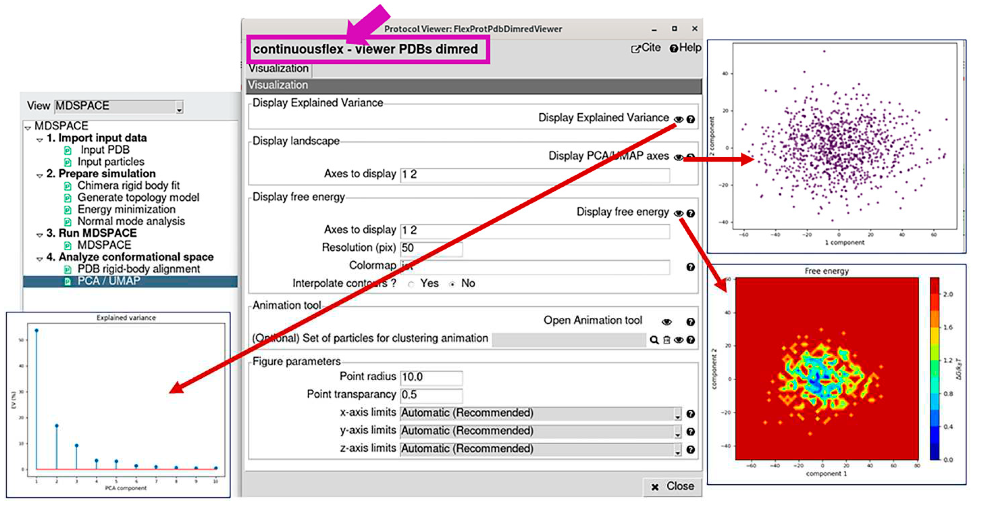
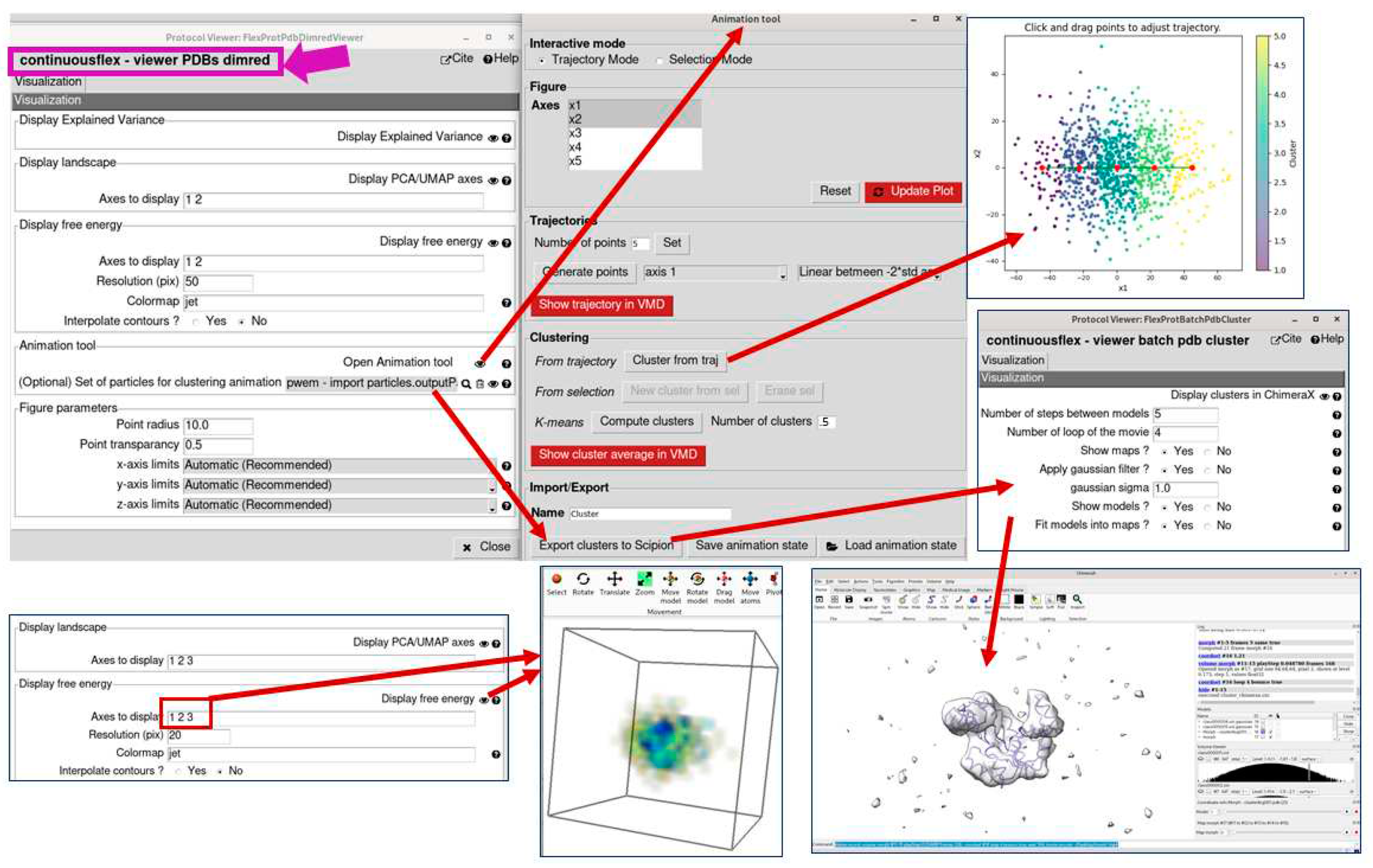
3.4. Analyze conformational space

To analyze the conformational space populated by the models obtained in Step 3 (the models fitted to the data), these models can be projected onto a low-dimensional space using PCA or UMAP dimension reduction methods. Before PCA (“PCA” box in Figure 1B,C) or UMAP (“UMAP” box in Figure 1B,C), the models should be rigid-body aligned (e.g., with respect to the initial conformation) to discard the rigid-body motions introduced during the MD simulation (‘Rigid body align” box in Figure 1B,C).

The “PCA / UMAP” results can be visualized and analyzed by opening the corresponding viewer, by first clicking on the “PCA” or “UMAP” box (Figure 1B,C) and, then, on the red “Analyse Results” button. This viewer allows displaying the variance explained by the different PCA axes (Figure 5), the conformational and free energy landscapes (in up to 3 dimensions) by specifying the PCA/UMAP axes to display (Figure 5 and Figure 6), atomic motion trajectories along different directions in this space (principal axes or a free-hand trajectories) by using “Open Animation Tool” (Figure 6), and clustering the points in this space (Figure 6) along the different directions automatically (clusters linearly distributed along a specified direction or obtained by K-means clustering) or by manual selection of points. The clusters can be exported into the Scipion project (Figure 6) to calculate 3D average density maps from the clusters (3D reconstructions when analyzing images and subtomogram averages when analyzing subtomograms). The average density maps and the average atomic models obtained from the clusters can be visualized using the corresponding viewer (by first clicking on the box related to the exported clusters and, then, on the red “Analyse Results” button). This clusters-related viewer allows displaying ChimeraX animations of the trajectory of the average atomic models superposed with the trajectory of the average density maps. This animation can be saved in MP4 video file format via the ChimeraX command-line section.

4. Discussion

In this article, we described the software with graphical interface and the basic workflow templates for running MDSPACE and MDTOMO hybrid methods, which are available in ContinuousFlex software package. The MDSPACE and MDTOMO methods combine NMMD (normal mode molecular dynamics) simulations with data analysis to extract the continuous conformational variability information and the full conformational landscapes of biomolecules from their cryo-EM single particle images and cryo-ET subtomograms. The performance of MDSPACE and MDTOMO were shown in our previous work using synthetic and experimental data. This article presents the tools that should facilitate a broader usage of these two recently developed methods. We hope that this article will be valuable to many cryo-EM practitioners.

Author Contributions

Conceptualization, R.V., M.H., I.H. and S.J.; Methodology, R.V., M.H., I.H. and S.J.; Software, R.V., M.H. and I.H.; Validation, R.V. and S.J.; Resources, S.J.; Writing – Original Draft Preparation, S.J. and R.V.; Writing – Review & Editing, R.V., M.H., I.H. and S.J.; Supervision, S.J.; Project Administration, S.J.; Funding Acquisition, S.J.

Funding

We acknowledge the support of the French National Research Agency - ANR (ANR-19-CE11-0008 and ANR-20-CE11-0020-03); the cooperation between the CNRS and the University of Melbourne (The Melbourne-CNRS Network, PRC 2889, CNRS 80 Prime); and access to HPC resources of CINES and IDRIS granted by GENCI (A0100710998R, A0100710998, A0070710998, AP010712190, AD011012188).

Data Availability Statement

The source code of ContinuousFlex is available at https://github.com/scipion-em/scipion-em-continuousflex. The instructions for ContinuousFlex software installation and a detailed tutorial for running MSPACE and MDTOMO methods, together with test datasets are available at https://zenodo.org/doi/10.5281/zenodo.10051882. The ContinuousFlex installation instructions also include the instructions for installing Scipion, Xmipp, ChimeraX, and VMD, which are required for using ContinuousFlex. Further questions regarding the software or data availability can be addressed to the corresponding author.

Conflicts of Interest

The authors declare no conflict of interest.

References

Svidritskiy E, Brilot AF, Koh CS, Grigorieff N, Korostelev AA. Structures of yeast 80S ribosome-tRNA complexes in the rotated and nonrotated conformations. Structure. 2014, 22, 1210–1218.
Zhou A, Rohou A, Schep DG, Bason JV, Montgomery MG, Walker JE, et al. Structure and conformational states of the bovine mitochondrial ATP synthase by cryo-EM. Elife. 2015, 4, e10180.
Bai XC, Rajendra E, Yang G, Shi Y, Scheres SH. Sampling the conformational space of the catalytic subunit of human gamma-secretase. Elife. 2015, 4.
Abeyrathne PD, Koh CS, Grant T, Grigorieff N, Korostelev AA. Ensemble cryo-EM uncovers inchworm-like translocation of a viral IRES through the ribosome. Elife. 2016, 5.
Banerjee S, Bartesaghi A, Merk A, Rao P, Bulfer SL, Yan Y, et al. 2.3 A resolution cryo-EM structure of human p97 and mechanism of allosteric inhibition. Science. 2016, 351, 871–875.
Hofmann S, Januliene D, Mehdipour AR, Thomas C, Stefan E, Brüchert S, et al. Conformation space of a heterodimeric ABC exporter under turnover conditions. Nature. 2019, 571, 580–583.
Nakane T, Kotecha A, Sente A, McMullan G, Masiulis S, Brown PMGE, et al. Single-particle cryo-EM at atomic resolution. Nature. 2020, 587, 152–156.
Kato K, Miyazaki N, Hamaguchi T, Nakajima Y, Akita F, Yonekura K, et al. High-resolution cryo-EM structure of photosystem II reveals damage from high-dose electron beams. Communications Biology. 2021, 4, 382.
Schur FK, Obr M, Hagen WJ, Wan W, Jakobi AJ, Kirkpatrick JM, et al. An atomic model of HIV-1 capsid-SP1 reveals structures regulating assembly and maturation. Science. 2016, 353, 506–508.
Wan W, Kolesnikova L, Clarke M, Koehler A, Noda T, Becker S, et al. Structure and assembly of the Ebola virus nucleocapsid. Nature. 2017, 551, 394–397.
Himes BA, Zhang P. emClarity: software for high-resolution cryo-electron tomography and subtomogram averaging. Nature Methods. 2018, 15, 955–961.
von Kügelgen A, Tang H, Hardy GG, Kureisaite-Ciziene D, Brun YV, Stansfeld PJ, et al. In Situ Structure of an Intact Lipopolysaccharide-Bound Bacterial Surface Layer. Cell. 2020, 180, 348–358.
Scheres SH, Gao H, Valle M, Herman GT, Eggermont PP, Frank J, et al. Disentangling conformational states of macromolecules in 3D-EM through likelihood optimization. Nat Methods. 2007, 4, 27–29.
Scheres SH. RELION: implementation of a Bayesian approach to cryo-EM structure determination. J Struct Biol. J Struct Biol. 2012, 180, 519–530. [CrossRef] [PubMed]
Lyumkis D, Brilot AF, Theobald DL, Grigorieff N. Likelihood-based classification of cryo-EM images using FREALIGN. J Struct Biol. 2013, 183, 377–388.
Punjani A, Rubinstein JL, Fleet DJ, Brubaker MA. cryoSPARC: algorithms for rapid unsupervised cryo-EM structure determination. Nature methods. 2017, 14, 290–296.
Kimanius D, Dong L, Sharov G, Nakane T, Scheres SHW. New tools for automated cryo-EM single-particle analysis in RELION-4.0. Biochem J. 2021, 478, 4169–4185.
Scheres SHW, Melero R, Valle M, Carazo J-M. Averaging of Electron Subtomograms and Random Conical Tilt Reconstructions through Likelihood Optimization. Structure. 2009, 17, 1563–1572.
Stölken M, Beck F, Haller T, Hegerl R, Gutsche I, Carazo J-M, et al. Maximum likelihood based classification of electron tomographic data. Journal of Structural Biology. 2011, 173, 77–85.
Bharat TAM, Scheres SHW. Resolving macromolecular structures from electron cryo-tomography data using subtomogram averaging in RELION. Nature Protocols. 2016, 11, 2054–2065.
Jin Q, Sorzano COS, De La Rosa-Trevín JM, Bilbao-Castro JR, Núñez-Ramírez R, Llorca O, et al. Iterative elastic 3D-to-2D alignment method using normal modes for studying structural dynamics of large macromolecular complexes. Structure. 2014, 22, 496–506.
Dashti A, Schwander P, Langlois R, Fung R, Li W, Hosseinizadeh A, et al. Trajectories of the ribosome as a Brownian nanomachine. Proc Natl Acad Sci U S A. 2014, 111, 17492–17497.
Moscovich A, Halevi A, Andén J, Singer A. Cryo-EM reconstruction of continuous heterogeneity by Laplacian spectral volumes. Inverse Problems. 2020, 36, 024003.
Lederman RR, Andén J, Singer A. Hyper-molecules: on the representation and recovery of dynamical structures for applications in flexible macro-molecules in cryo-EM. Inverse Problems. 2020, 36, 044005.
Chen M, Ludtke SJ. Deep learning-based mixed-dimensional Gaussian mixture model for characterizing variability in cryo-EM. Nature Methods. 2021, 18, 930–936.
Punjani A, Fleet DJ. 3D variability analysis: Resolving continuous flexibility and discrete heterogeneity from single particle cryo-EM. Journal of Structural Biology. 2021, 213, 107702.
Zhong ED, Bepler T, Berger B, Davis JH. CryoDRGN: reconstruction of heterogeneous cryo-EM structures using neural networks. Nature Methods. 2021, 18, 176–185.
Zhong ED, Lerer A, Davis JH, Berger B. CryoDRGN2, Ab initio neural reconstruction of 3D protein structures from real cryo-EM images. 2021 IEEE/CVF International Conference on Computer Vision (ICCV)2021. p. 4046-55.
Levy A, Wetzstein G, Martel J, Poitevin F, Zhong ED. Amortized Inference for Heterogeneous Reconstruction in Cryo-EM. Adv Neural Inf Process Syst. 2022, 35, 13038–13049.
Hamitouche I, Jonic S. DeepHEMNMA: ResNet-based hybrid analysis of continuous conformational heterogeneity in cryo-EM single particle images. Front Mol Biosci. 2022, 9, 965645.
Punjani A, Fleet DJ. 3DFlex: determining structure and motion of flexible proteins from cryo-EM. Nature Methods. 2023, 20, 860–870.
Herreros D, Lederman RR, Krieger JM, Jiménez-Moreno A, Martínez M, Myška D, et al. Estimating conformational landscapes from Cryo-EM particles by 3D Zernike polynomials. Nature Communications. 2023, 14, 154.
Vuillemot R, Mirzaei A, Harastani M, Hamitouche I, Fréchin L, Klaholz BP, et al. MDSPACE: Extracting Continuous Conformational Landscapes from Cryo-EM Single Particle Datasets Using 3D-to-2D Flexible Fitting based on Molecular Dynamics Simulation. J Mol Biol. 2023, 435, 167951.
Harastani M, Eltsov M, Leforestier A, Jonic S. HEMNMA-3D: Cryo Electron Tomography Method Based on Normal Mode Analysis to Study Continuous Conformational Variability of Macromolecular Complexes. Frontiers in molecular biosciences. 2021, 8, 663121.
Vuillemot R, Rouiller I, Jonić S. MDTOMO method for continuous conformational variability analysis in cryo electron subtomograms based on molecular dynamics simulations. Scientific Reports. 2023, 13, 10596.
Harastani M, Eltsov M, Leforestier A, Jonic S. TomoFlow: Analysis of continuous conformational variability of macromolecules in cryogenic subtomograms based on 3D dense optical flow. Journal of molecular biology. 2022, 434, 167381.
Powell BM, Davis JH. Learning structural heterogeneity from cryo-electron sub-tomograms with tomoDRGN. bioRxiv. 2023.
Tagare HD, Kucukelbir A, Sigworth FJ, Wang H, Rao M. Directly reconstructing principal components of heterogeneous particles from cryo-EM images. Journal of structural biology. 2015, 191, 245–262.
Katsevich E, Katsevich A, Singer A. Covariance Matrix Estimation for the Cryo-EM Heterogeneity Problem. SIAM J Imaging Sci. 2015, 8, 126–185.
Liao Hstau Y, Hashem Y, Frank J. Efficient Estimation of Three-Dimensional Covariance and its Application in the Analysis of Heterogeneous Samples in Cryo-Electron Microscopy. Structure. 2015, 23, 1129–1137.
Marshall NF, Mickelin O, Shi Y, Singer A. Fast principal component analysis for cryo-electron microscopy images. Biological Imaging. 2023, 3, e2.
Tama F, Miyashita O, Brooks CL. Flexible Multi-scale Fitting of Atomic Structures into Low-resolution Electron Density Maps with Elastic Network Normal Mode Analysis. Journal of Molecular Biology. 2004, 337, 985–999.
Orzechowski M, Tama F. Flexible fitting of high-resolution x-ray structures into cryoelectron microscopy maps using biased molecular dynamics simulations. Biophysical journal. 2008, 95, 5692–5705.
Miyashita O, Kobayashi C, Mori T, Sugita Y, Tama F. Flexible fitting to cryo-EM density map using ensemble molecular dynamics simulations. Journal of computational chemistry. 2017, 38, 1447–1461.
Miyashita O, Tama F. Hybrid Methods for Macromolecular Modeling by Molecular Mechanics Simulations with Experimental Data. Adv Exp Med Biol. 2018, 1105, 199–217.
Vuillemot R, Miyashita O, Tama F, Rouiller I, Jonic S. NMMD: Efficient cryo-EM flexible fitting based on simultaneous Normal Mode and Molecular Dynamics atomic displacements. Journal of Molecular Biology. 2022, 434, 167483.
Harastani M, Vuillemot R, Hamitouche I, Barati Moghadam N, Jonic S. ContinuousFlex: Software package for analyzing continuous conformational variability of macromolecules in cryo electron microscopy and tomography data. Journal of Structural Biology. 2022, 107906.
Conesa P, Fonseca YC, Jiménez de la Morena J, Sharov G, de la Rosa-Trevín JM, Cuervo A, et al. Scipion3, A workflow engine for cryo-electron microscopy image processing and structural biology. Biological Imaging. 2023, 3, e13.
De la Rosa-Trevín J, Quintana A, Del Cano L, Zaldívar A, Foche I, Gutiérrez J, et al. Scipion: A software framework toward integration, reproducibility and validation in 3D electron microscopy. Journal of structural biology. 2016, 195, 93–99.
Jiménez de la Morena J, Conesa P, Fonseca YC, de Isidro-Gómez FP, Herreros D, Fernández-Giménez E, et al. ScipionTomo: Towards cryo-electron tomography software integration, reproducibility, and validation. Journal of Structural Biology. 2022, 214, 107872.
Herreros D, Krieger JM, Fonseca Y, Conesa P, Harastani M, Vuillemot R, et al. Scipion Flexibility Hub: an integrative framework for advanced analysis of conformational heterogeneity in cryoEM. Acta Crystallographica Section D. 2023, 79, 569–584.
Harastani M, Sorzano COS, Jonić S. Hybrid Electron Microscopy Normal Mode Analysis with Scipion. Protein Science. 2020, 29, 223–236.
Pearson K. LIII. On lines and planes of closest fit to systems of points in space. The London, Edinburgh, and Dublin Philosophical Magazine and Journal of Science. 1901, 2, 559–572.
McInnes L, Healy J, Melville J. UMAP: Uniform Manifold Approximation and Projection for Dimension Reduction. ArXiv. 2018, abs/1802.03426.
Kobayashi C, Jung J, Matsunaga Y, Mori T, Ando T, Tamura K, et al. GENESIS 1.1, A hybrid-parallel molecular dynamics simulator with enhanced sampling algorithms on multiple computational platforms. J Comput Chem. 2017, 38, 2193–2206.
Huang J, MacKerell Jr AD. CHARMM36 all-atom additive protein force field: Validation based on comparison to NMR data. Journal of computational chemistry. 2013, 34, 2135–2145.
Karanicolas J, Brooks CL. Improved Gō-like Models Demonstrate the Robustness of Protein Folding Mechanisms Towards Non-native Interactions. Journal of Molecular Biology. 2003, 334, 309–325.
Noel JK, Levi M, Raghunathan M, Lammert H, Hayes RL, Onuchic JN, et al. SMOG 2, A Versatile Software Package for Generating Structure-Based Models. PLoS computational biology2016. p. e1004794.
Suhre K, Sanejouand YH. ElNemo: a normal mode web server for protein movement analysis and the generation of templates for molecular replacement. Nucleic Acids Res. 2004, 32, W610–W614.
Goddard TD, Huang CC, Meng EC, Pettersen EF, Couch GS, Morris JH, et al. UCSF ChimeraX: Meeting modern challenges in visualization and analysis. Protein Science. 2018, 27, 14–25.
Humphrey W, Dalke A, Schulten K. VMD: visual molecular dynamics. J Mol Graph. 1996, 14, 33–38.

Figure 1. MDSPACE and MDTOMO workflow templates provided by ContinuousFlex. (A) MDSPACE and MDTOMO workflow templates are accessible via the Scipion menu “Others” -> “Import workflow template”. (B) MDSPACE workflow template. (C) MDTOMO workflow template. The MDSPACE and MDTOMO workflows are globally the same, but they analyze different types of data (2D single particle images and 3D subtomograms, respectively).

Figure 2. Topology model (force field type) and energy minimization graphical interface. (A) Topology model generation using all-atom CHARMM or Cα-atom-based Gō models (the interface also allows using all-atom Gō model). (B) Energy minimization of the model generated in (A) before calculating normal modes and data analysis with NMMD simulations (“Simulation type” in the “Simulation” tab is set to “Minimization”). The default values of the parameters and options in the tabs of the “Energy Minimization” interface can be kept unchanged (the full documentation on the simulation parameters can be found at the GENESIS website, https://www.r-ccs.riken.jp/labs/cbrt). .

Figure 3. Data analysis using NMMD simulations (corresponding to the “MDSPACE”/”MDTOMO” box in Figure 1B,C). (A) “Simulation” tab, which allows choosing the simulation type, the integrator, and its parameters. Here, NMMD is selected, which additionally allows selecting normal modes and their parameters that will be used within NMMD (note that NMMD integrates over time atomic coordinates and normal-mode amplitudes and it performs this numerical integration using “Velocity Verlet” integrator available in GENESIS). (B) “MD parameters” tab, which allows specifying additional MD simulation parameters (see the main text). (C) “EM data” tab, which allows specifying the type of the data to analyze (“Cryo-EM flexible fitting” allows choosing “Image(s)” or “Volume(s)”, for analyzing single particle images or cryo electron subtomograms, respectively), the dataset (“Image Parameters” section, which allows choosing the set of single particle images or subtomograms that will be analyzed, its initial rigid-body alignment parameters, and pixel/voxel size), and the biasing force parameters (“Fitting Parameters” section). (D) “Refinement”, “Inputs”, and “MPI parallelization” tabs, which allow specifying other parameters, like the number of iterations and the number of PCA components for the iterative conformation-space refinement, the model to initiate the simulation, and the parallelization resources. For more details on the available integrators and MD-related simulation parameters, see the GENESIS documentation, https://www.r-ccs.riken.jp/labs/cbrt.

Figure 4. Analysis of results of data analysis using NMMD simulations (corresponding to the “MDSPACE”/”MDTOMO” box in Figure 1B,C). The viewer allows displaying statistical analysis of the energy, cross-correlation (CC), normal mode amplitudes, and root mean square deviation (RMSD) trajectories over a selected set of particle images or subtomograms (“Simulation selection”). Also, for one selected particle image or subtomogram, it allows displaying the initial and final 3D structures with ChimeraX (“Display results in Chimerax”) and animating the trajectory of atomic coordinates over the simulation with VMD (“Display trajectory in VMD”).

Figure 5. PCA/UMAP results viewer. It allows displaying the variance explained by the different PCA axes, the conformational and free energy landscapes (in up to 3 dimensions) by specifying the PCA/UMAP axes to display, and access to “Open Animation Tool” for animating the atomic motion trajectories along different directions and clustering the points in this space (see also Figure 6).

Figure 6. Results of using “Open Animation Tool” in the PCA/UMAP results viewer (see also Figure 5). It allows displaying the atomic motion trajectories along different directions in this space (principal axes or a free-hand trajectories) and clustering the points in the PCA/UMAP space along the different directions automatically (clusters linearly distributed along a specified direction or obtained by K-means clustering) or by manual selection of points. The clusters can be exported into the Scipion project to calculate 3D average density maps from the clusters (3D reconstructions in the case of analyzing images and subtomogram averages in the case of analyzing subtomograms). The interface also allows automatic ChimeraX animations of the superposed average atomic models and density maps from the clusters. These animations can be saved in MP4 video file format (ChimeraX command line).

Disclaimer/Publisher’s Note: The statements, opinions and data contained in all publications are solely those of the individual author(s) and contributor(s) and not of MDPI and/or the editor(s). MDPI and/or the editor(s) disclaim responsibility for any injury to people or property resulting from any ideas, methods, instructions or products referred to in the content.

© 2023 by the authors. Licensee MDPI, Basel, Switzerland. This article is an open access article distributed under the terms and conditions of the Creative Commons Attribution (CC BY) license (http://creativecommons.org/licenses/by/4.0/).

Copyright: This open access article is published under a Creative Commons CC BY 4.0 license, which permit the free download, distribution, and reuse, provided that the author and preprint are cited in any reuse.