1. Introduction
Artificial intelligence (AI) and Machine Learning (ML) are two related terms in computer science and technology. Although they are related, their definitions are not interchangeable. While AI refers to creating machines that perform tasks that typically require human intelligence, such as perception, reasoning, learning, and decision-making, ML is only a subset of AI that involves training algorithms to learn patterns in data and make predictions or decisions based on them. AI is, therefore, a much broader concept encompassing various fields of study, such as computer vision, natural language processing, robotics, and more. Additionally, Machine Learning focuses on developing algorithms and statistical models that can analyze data and predict, interpret or decide [
1]. AI typically uses a rule-based approach, where systems are programmed with a set of rules and instructions to follow. Machine Learning, on the other hand, uses a data-driven approach, where algorithms learn from data to identify patterns and make predictions. AI systems are typically designed and programmed by humans, while Machine Learning algorithms are trained on data [
2]. Machine Learning algorithms require large amounts of data to be trained effectively, whereas AI systems can be designed with a smaller set of rules and instructions [
1].
There are three main types of Machine Learning: supervised learning, unsupervised learning, and reinforcement learning. In supervised learning, the algorithm is trained on a labelled dataset to predict an output given an input [
3]. In unsupervised learning, the algorithm identifies patterns and structures in an unlabeled dataset. In semi-supervised learning, the algorithm is trained on a combination of labelled and unlabeled data. Finally, in reinforcement learning, the algorithm learns to make decisions by interacting with an environment and receiving feedback in the form of rewards or penalties [
4]. Each type of Machine Learning has its strengths and weaknesses, and the choice of which type to use depends on the nature of the problem and the available data [
5]. Neural Networks (
) and Adaptive Neuro-Fuzzy Inference Systems (ANFIS) are two types of supervised ML. A Fuzzy approach can be applied in supervised and unsupervised classifications as a mathematical framework [
6,
7].
Fuzzy Logic (FL), developed by Zadeh [
8], is an approach for dealing with imprecise or uncertain data often encountered in real-world applications. FL provides a way to handle linguistic variables and Fuzzy sets, delegating and manipulating imprecise or ambiguous data. It provides a set of rules for making decisions or predictions based on this data and allows for more flexible and nuanced reasoning than traditional Boolean logic [
9]. FL has been used in various fields, including control systems, pattern recognition, and decision-making. For example, FL has been used to control the speed of electric motors in industrial processes, to diagnose medical conditions based on symptoms, and to make decisions in financial forecasting [
10].
FL has been used in various fields, including structural studies. FL provides a framework for dealing with imprecise or uncertain data, often encountered in structural studies. FL allows for more flexible and nuanced reasoning, making it an attractive tool for analyzing complex structural systems. FL has been applied in structural studies in assessing seismic hazards and estimating earthquake probability and potential consequences. FL combined data from multiple sources, such as seismic data, geological information, and historical earthquake data, to generate a comprehensive seismic hazard assessment [
11]. FL was also utilized to design and analyze structural systems to model the performance of complex systems, such as buildings, bridges, and other infrastructure, including optimizing the design of reinforced concrete structures [
12]. FL can be used to analyze data from multiple sensors, such as strain gauges and accelerometers, to detect changes in the structural performance that may indicate damage or deterioration [
13]. Another type of utilization was for parametric evaluation of dry concrete joints to continuously evaluate the joints with different parameter ratios. At the same time, the limited number of the tests can be generally managed, which will, without ML, end to discrete data [
14].
Neural Networks (
), a supervised technique, has been increasingly used in various fields, including structural studies. Using Neural Networks in structural studies can lead to more accurate and reliable analyses and help ensure the safety and reliability of critical infrastructure. Structural health assessment is one area where Neural Networks have been applied in structural studies. Structural health assessment involves monitoring the condition of structures, such as bridges and buildings, to detect any defects or damage. Neural Networks can be used to analyze data from multiple sensors, such as strain gauges and accelerometers, to detect changes in the structural performance that may indicate damage or deterioration [
15]. Neural Networks have also been used to design and optimize structural systems. It was utilized to model the performance of complex systems, such as buildings, bridges, and other infrastructure, and to optimize their design based on performance criteria. For example, Neural Networks were utilized to optimize the design of steel-concrete composite structures [
16]. Another application of
in structural studies is in predicting structural performance under various loading conditions, trained on data from physical experiments or numerical simulations to predict the response of structural systems to different loads. Likewise,
to predict the deflection and stress of steel-concrete composite [
17].
Adaptive Neuro-Fuzzy Inference System (ANFIS) is another supervised ML approach, which is a type of ML algorithm that combines the strengths of Neural Networks and FL used in various fields, including structural studies such as in predicting the dynamic performance of structures under seismic loads. ANFIS can be trained on data from physical experiments or numerical simulations to predict the response of structural systems to seismic loads and the displacement and acceleration response of steel frame structures [
18]. ANFIS was also employed in the assessment of structural health. It can be used to analyze data from sensors, such as accelerometers and strain gauges, to detect structural defects or damage. For example, ANFIS has been used to detect damage in reinforced concrete structures based on data from acoustic emissions [
19]. Another application in structural studies is in the design and optimization of structural systems. ANFIS can model the performance of complex systems, such as buildings and bridges, and optimize their design based on performance criteria. For example, ANFIS was used to optimize the design of steel-concrete composite beams [
20].
Reinforced concrete is a widely used construction material in structural engineering due to its strength and durability. However, predicting the performance of reinforced concrete structures is a complex task, as it depends on various factors such as material properties, geometry, and loading conditions. FL, Neural Network, and ANFIS are three Machine Learning techniques that can be used in reinforced concrete research to accurately predict these structures’ behaviour. For instance - FL is utilized to model the mechanical behaviour of concrete structures under different loading conditions and predict the deflection of reinforced concrete beams [
21]. - Neural Networks can be trained on large datasets to identify complex patterns and relationships between input and output variables, predicting the compressive strength of concrete based on various input parameters [
22]. - ANFIS has been used in reinforced concrete research to predict various properties of concrete structures, such as the compressive strength, flexural performance, and shear strength, along with predicting the performance of reinforced concrete beams with different reinforcement [
23,
24].
Despite their potential, several challenges must be addressed to apply the ML approach practically. Some primary challenges can be mentioned: 1. Lack of engineers’ familiarity with this method and difficulty in modelling complex relationships; 2- Lack of awareness about the differences in performance of different ML techniques to a wise tool selection. 3- Sensitivity of these techniques to the size of a table, number of parameters and type of relation between the input and outputs (linear and nonlinear). 4- Machine Learning models are often called "black boxes" because they can produce complex and non-intuitive results. This makes it challenging for engineers to interpret and explain the outputs of the models; in other words, the designers do not know up to which stand these methods are trustworthy. 5- the studies in which the ML approaches were used are mainly based on the researches and experimental data, while direct comparisons between the standard known calculations and ML’s results are needed.
In this regard, the current paper aims to discuss the three types of Machine Learning, including Fuzzy, and ANFIS, to re-introduce and compare their performances in one example. In the case study, the Standard calculation of a concrete beam was selected, which is known to the engineer. This discussion discussed the sensitivity of the methods to the number of parameters and the size of the table. Additionally, the accuracy of all methods with each other and routine calculations was compared.
2. Discussion
2.1. Initialization
Coding, Standard Beam Section Calculation
This paper aims to evaluate the performance of ML operators in delegating the standard structural computing process. As the case study, a wide range of structural subjects and Standards can be selected for analyzing or designing steel and concrete elements. Here, the known designing process of concrete beams (
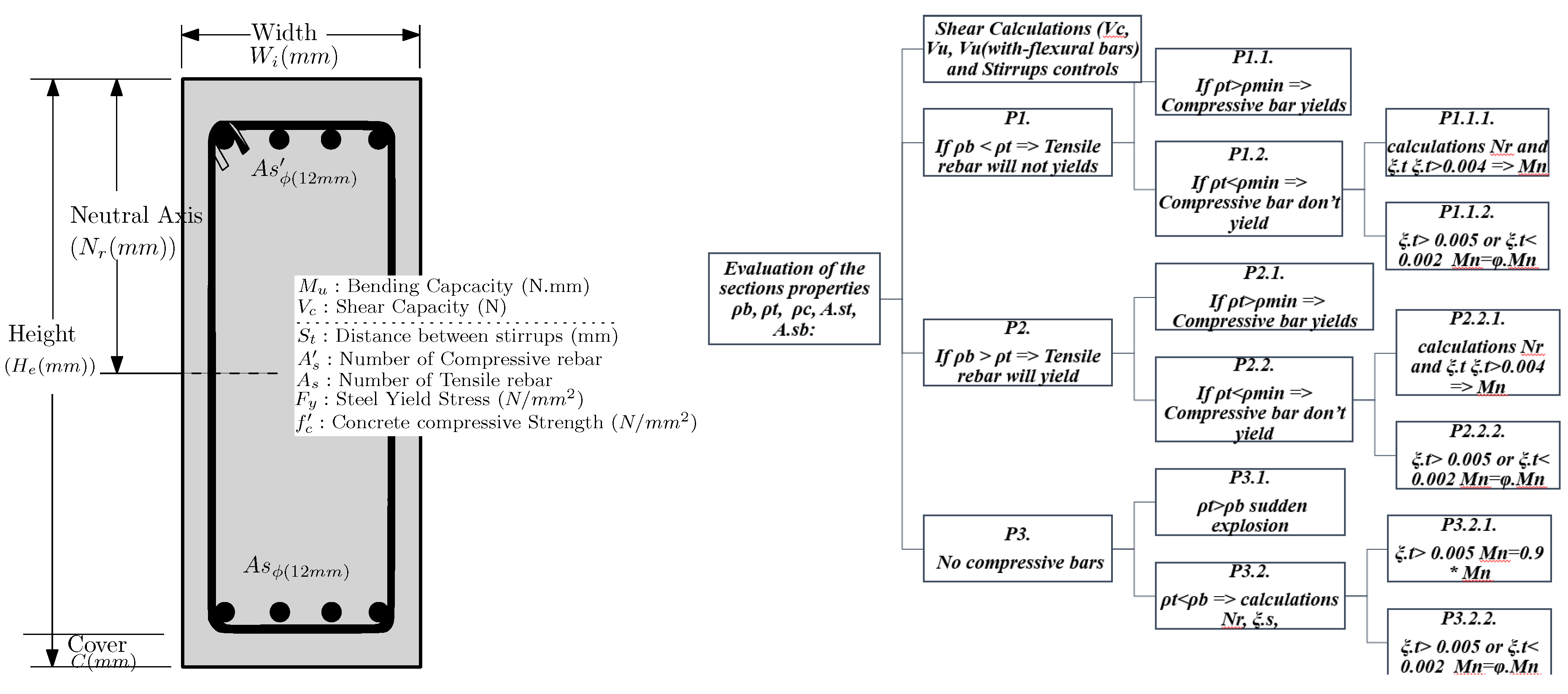
Figure 1) was chosen as the subject of interest, and in particular, the calculations of the beams’ bending and shear capacity were defined as the output (referring to
[
25] standard), whereas features of the section were the adjustable parameters (
Figure 1) in the codes. In these calculations, after initialization and some basic calculations such as section area (
A), amount of compressive and tensile re-bars,
and their percentages
along with beam re-bar balance percentage
were calculated.
Simple algorithmic codes were developed in MATLAB to calculate ACI and parametrically calculate the capacities. The shear calculation regarding steel (stirrups) and concrete capacities was managed in one step. The shear capacity (
is
of the steel and concrete capacities summation. The bending performance of the section was divided into three different steps.
Figure 1 shows that the bending performances based on the comparison between
and availability of compressive re-bar get divided into three different performance types (
).
In the following process, comparison with available and minimum allowed re-bar categorizes the section to other subcategories . This category indicates the type of Standard formulas for calculating neutral lines and capacities of each type of section. Finally, a comparison between the amounts of the calculated strains indicates some coefficients which, based on the standard, should be multiplied by the bending results. Numbers showed this last step of calculations as (). Finally, the following discussions interfaced the standard codes as a MATLAB function to all ML operations.
The results of several series of parametric calculations will produce different databases (
table) to be inferred with operators, and the operators’ results will be compared to the direct ACI coding. The aim of the study is not to discuss the performance of the beams, and the accuracy of the parametric calculations results is not decisive. Nonetheless, to have a practical example, the accuracy of the coded ACI function was compared to other references.
Table 1 compares the codes’ results and calculated amounts in references. Although not all of the references use ACI, the results displayed similar results for shear and bending capacities, proving the accuracy of the coded ACI and the similarity between the referenced standards.
The selection properties, including the Height (
) and Width (
), besides concrete and steel properties along with the steel mounts, are shown in the first row of
Table 1. The
in this Table shows the depth of the neutral line, calculated by codes and references for bending calculations. In selection, examples with different performance types were selected. For instance, the bending capacity of the first section (No.1 Table,
Table 1), by the codes and in the reference, are 7.1
e08
N.
mm and 7.08
e08
N.
mm. Likewise, the comparison of shear capacities in example 6 shows 3.53
N and 3.5
N. Generally, it was shown that the maximum difference between the results of the codes and references is
, proving the accuracy of the codes.
Coding, the Machine Learning Operators
Despite the different parameters for tuning, Machine Learning operators can be selected due to the limitation of the size of the paper, and the focus of the current study does not intensely discuss other possible variants of Coding. The codes were initially developed by other researchers/engineers and, alone as a possibility, were selected to prepare an overview for the structural engineers. This study aims to give an outline to the structural engineer for finding the solution for the desirable interpretation of their numerical and experimental results and does not aim to propose the best commands; the developed codes in this study can further researchers be replaced by other programming languages or can be optimized for promoting their performances. Alone, some parts of the developed MATLAB codes to give an overview will be briefly mentioned in each section.
2.2. Problem Definitions (Preparation of Look-up Table)
For discussing different ML techniques, all following sections use the proved codes as a MATLAB function called . This function can para-metrically calculate different ranges of the variables based on ACI. It imports all of the section parameters, including Height(), Width (), concrete compressive strength (, steel yield strength ()), Compressive re-bar ()), tensile re-bar ()) and calculates the shear ( and bending capacity ().
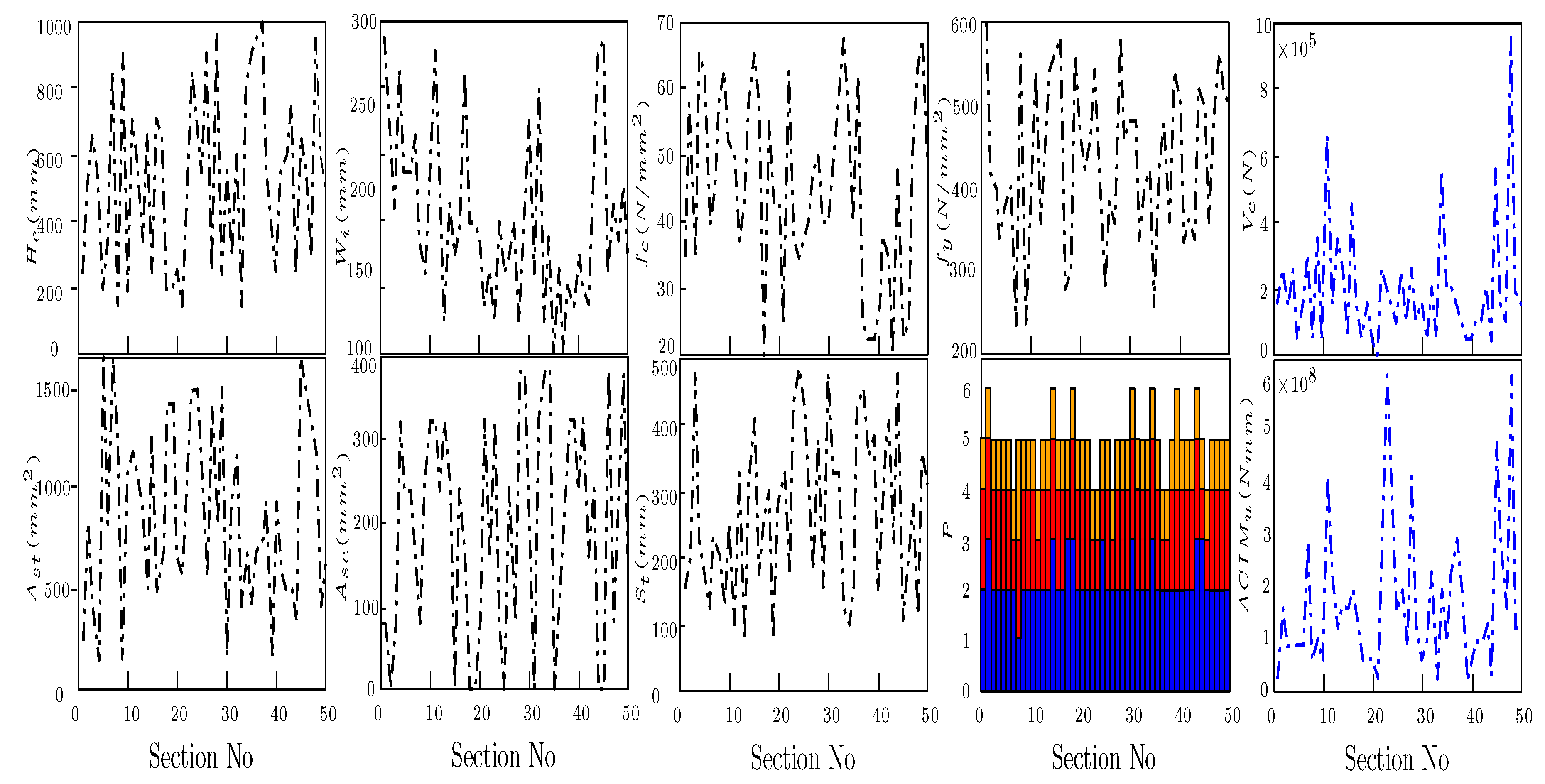
Figure 2 shows a series of analyses, including the properties of 50 different beam sections. The input was produced randomly (
) but in a specific range for each variable (
Table 2). The influences of these variables on the bending and shear capacities can be found in the last blue diagrams. The type of performance in the bar chart (
P) is shown in blue, red and orange. For instance, the first section displayed 2 for the Height of blue and red also 1 for the orange part on top of the bar, which means the performance of it belongs to category (2.2.1). It displays the tensile re-bar yields, compressive does not yield, and the strain is higher than 0.004 (Chart in
Figure 1).
In addition to the parameter and the ranges, demands two other criteria. The first criterion informs about the number of parameters selected in each calculation series (). It means all different features of the section can be selected parametrically (i.e. ) or just some (e.g. ). The second criterion is the size of the table () or, in other words, the number of calculated sections. The number of parameters () and the size of the table () as the primary measure was regarded for dissecting the performances of ML Operator () in the following sections. An MLO, which can delegate the results with higher accuracy and a lower amount of initial data (low ), has a more desirable performance. It would show its considerable importance when the difficulties in data production are considered. Indifferent filed, the data can be collected by quaternary (asking from experts), numerical analysis or experimental test, while in structural engineering, increasing the , especially in experimental studies, is complex and costly.
2.3. Parametric Evaluation of the Beams
In this study, beam capacity was selected as one of the easy structural calculations to evaluate the MLO. Likewise, can be used for independent parametric evaluations. It could also be connected to an optimization algorithm. Such a function, similar to software (e.g. SAP2000 Section Designer), can easily calculate the capacity of sections with different parameters. Hence, different operators can use it for multi-analysis to regard different aspects of the section’s performances and perform statistical evaluations and sensitivity analysis by MATLAB Simulink.
One simple evaluation without coding Sensitivity Analysis is evaluating the influence of each parameter on
&
.
Table 3, shows the influence of increasing the parameters twice (2.00) on this range’s bending and shear capacities. This evaluation showed that increasing the amount of all parameters twice increases the shear and bending capacity 7.18 times and 8.14 times. It means that bending capacity is more sensitive (No.1). That is, if the influences of stirrups are ignored despite no changes in increasing of
, the changes in
were reduced to 4.74 (No.2). It means in the selected range (
Table 2), distances between the stirrups influence the shear capacity up to
. The distance between the stirrups can not be due to the standard’s limitations (e.g. for keeping the ductility of beams) limitless changed, but the range was accepted as a parametric study.
In this range, Height has a similar influence on shear and bending and has a linear relation (No.3). Width has a higher effect on shear rather than bending (No.4). The changes in bending are not linear, and the width effect on bending in one step gets higher (due to changes in P). also shows a similar low influence on the and ; it means increasing the concrete properties regarding the in comparison to the changes in other parameters, such as high is not economical (No.5). Generally, the lowest influence was shown by compressive re-bar (No.7) and higher by Height and tensile re-bars (No.8).
3. Machine LEARNING Operatos (MLO)
To discuss the performance of the following MLO, the specific range is based on the expected dimensions and properties of the material used in all following investigations (
Table 2). In the prepared
table, the parameters linearly increased. Based on the ACI calculation, the first section selects Fuzzy Logic for delegating, interpreting, and using data (
table). Likewise, the Neural Network and ANFIS will repeat the same process. Additionally, their sensitivity to the size of
and
will be investigated. Finally, their performances regarding the different sizes of the
table and the number of parameters will be compared.
3.1. Fuzzy Log (FL)
Since MATLAB GUI caot generate codes to accept different ‘input’ and ‘output’ parameters, codes for making the interpreter of the table and were developed. In the membership function, two types of functions were regarded, including (‘trimf’ and ‘gaussmf’) to be adjusted by the operator (). Assigning the inputs to outputs for such a range of data was not effortless for making the rules. Hence, a ‘for’ loop based on the table was developed to develop adaptable codes for all essential parameters in designing the beams. In which the ‘1’ as the Variables and Weight for all rows of the Rule table was regarded. Then, the lookup table and ‘mamdani’ was used to make the ‘fis’ (. Furthermore, ‘input’, ‘output’ etc., by assigned to the ‘fis’, and finalized by adding the rules.
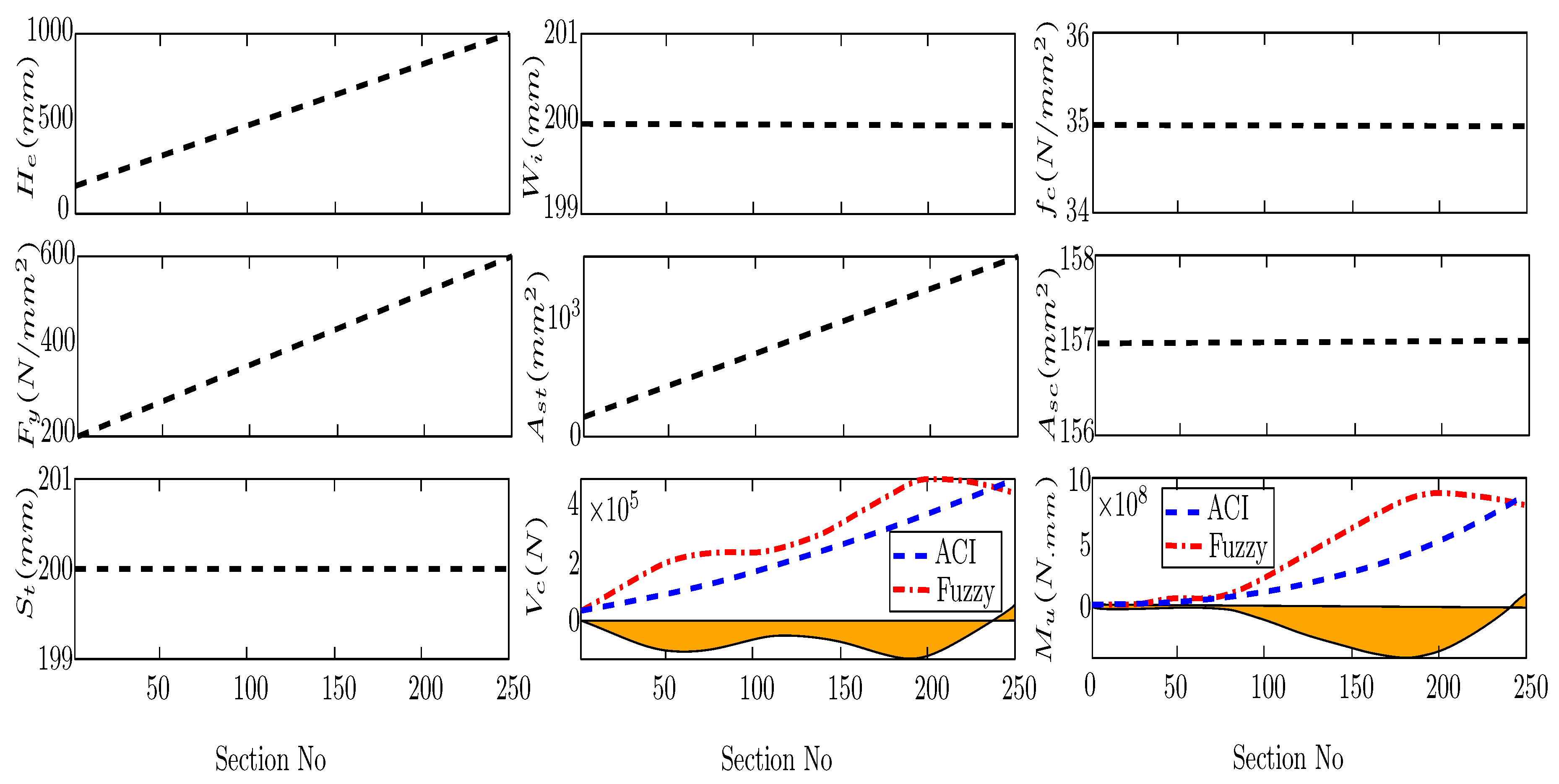
Figure 3 displays an example of the series of section calculations. In this example,
as the variables were selected, and 250 sections were calculated to make the
table (
). This Figure shows how the parameters change linearly to increase the bending and shear capacity based on ACI. The same input in Fuzzy, the
table, is used, and the two diagrams show the Fuzzy delegating results. In these diagrams, the flat parameters indicate the not chosen variable, which means the
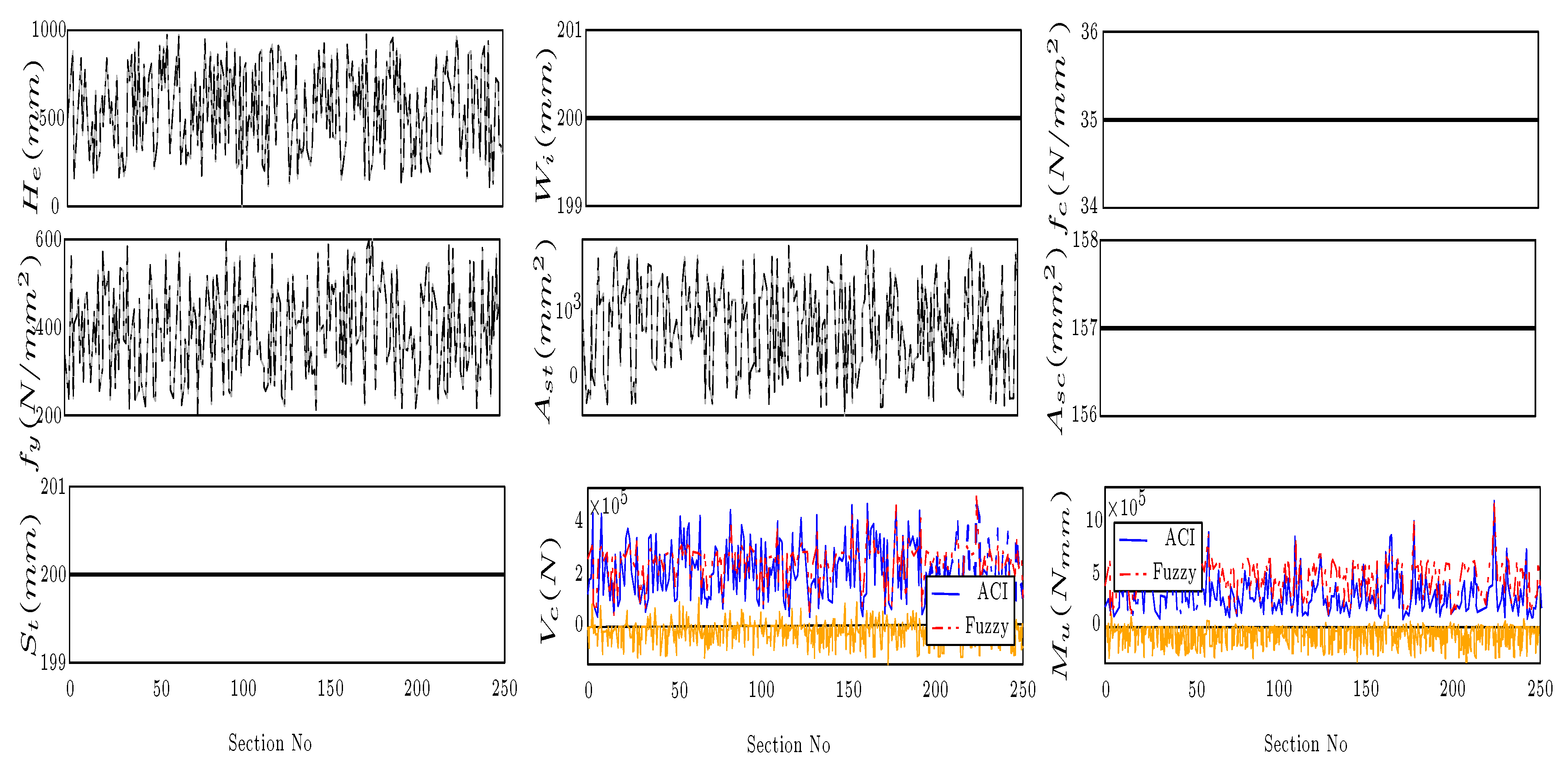
. The shown parameter in the last two diagrams, in blue, is the shear and bending capacity based on ACI. Likewise, red diagrams display the results of the Fuzzy operator. In these diagrams, the yellow bars are the difference between the targets (diversity between input from ACI codes and Fuzzy outputs). A similar example was made, utilizing randomized input and, accordingly, chaotic results of Fuzzy and ACI. This example shows the capacity of FL to interpret the not-sorted input. This capability shows its importance when several results of the studies against the current study regarding the type of the input parameters ca
ot be sorted,
Figure 4.
In another example in which just
as the variable and (
) as the table size was selected, the maximum Error (Differences between Fuzzy and Standard happened divided by the ACI capacities in each section), was limited to
. In this example, with three parameters, Error raised to
and
for the calculation of shear and bending, respectively, displaying a considerably low accuracy. In
Figure 3, the wave format of these Fuzzy diagrams and Errors shows that the error amount is not the same in different sections. The changes in Error are not related to beam section performance but come from the nature of Fuzzy. In another example with
parameter and
table size, the Error in shear and bending capacity was
, compared to the previous example with
table size is just
percent less accurate. It means up to some limits; despite its positive influence, increasing the size considerably raises the analyzing
, ca
ot significantly improve the accuracy. Nonetheless, adjusting the Fuzzy codes and changes in several parameters or the
table size can influence the results more. The influences of these adjusting components should be evaluated para-metrically.
Two more loops were added to the codes to evaluate the capability of adjusting the MLO. The first
loop operates the MLO by a different range of initial data in the
table. It means if the
is for instance 1208, ParsolutionSolution function, in the specific range calculates 1208, beam sections to be referenced by Fuzzy operator
. This evaluation shows how much data (including all parameters) is needed for the selected beam example. The other parameters, such as a nest (loop), were also regarded. This loop, in five different steps, changes the number of parameters. This additional
loop (PARA) in five different steps selects different parameters, decided based on the results of parametric evaluations (efficient of the parameter on the capacity),
Table 3. It was written by a
function, demanding
, general operations, while each one may have up to 2000, beam calculations.
.
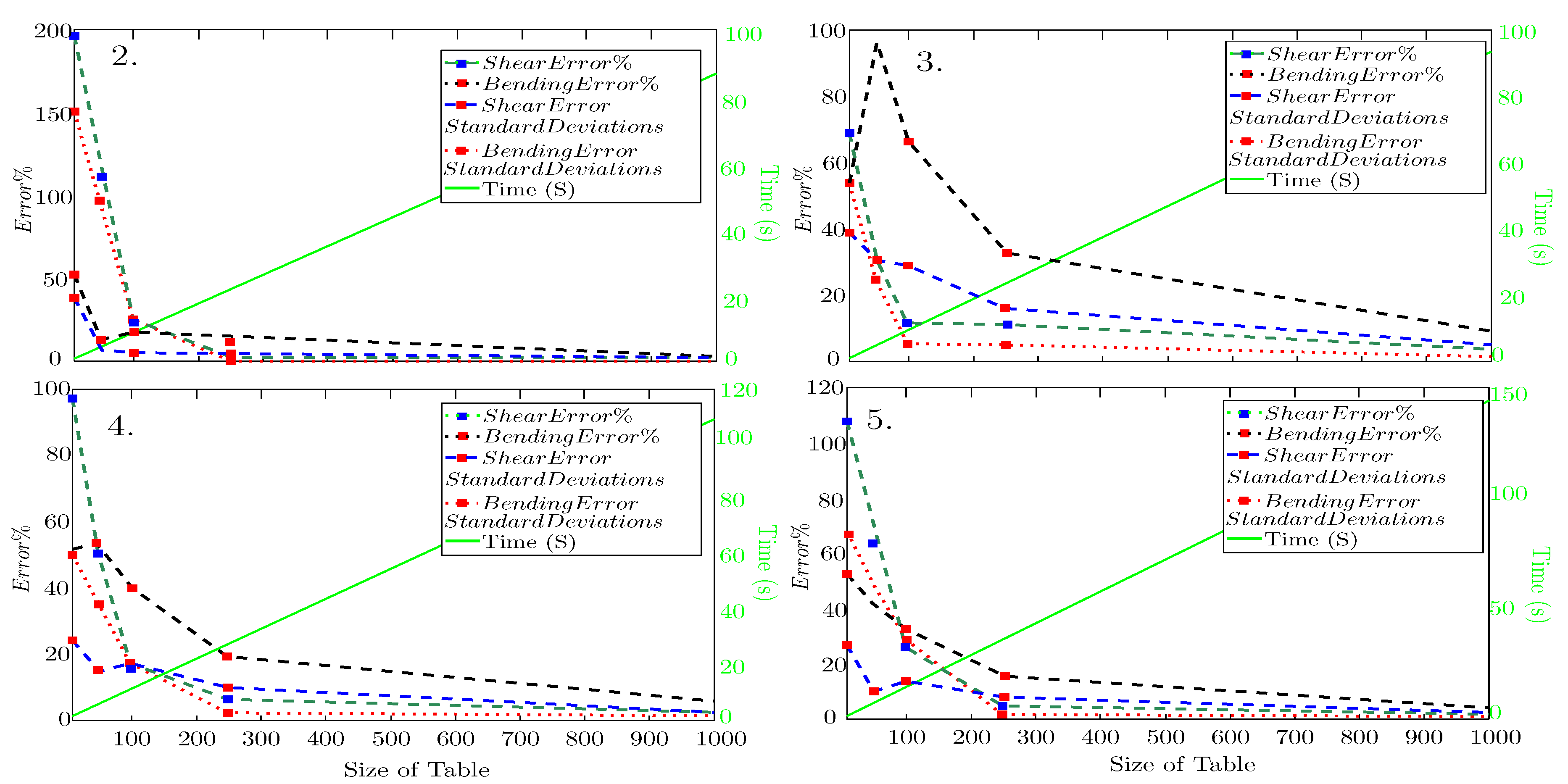
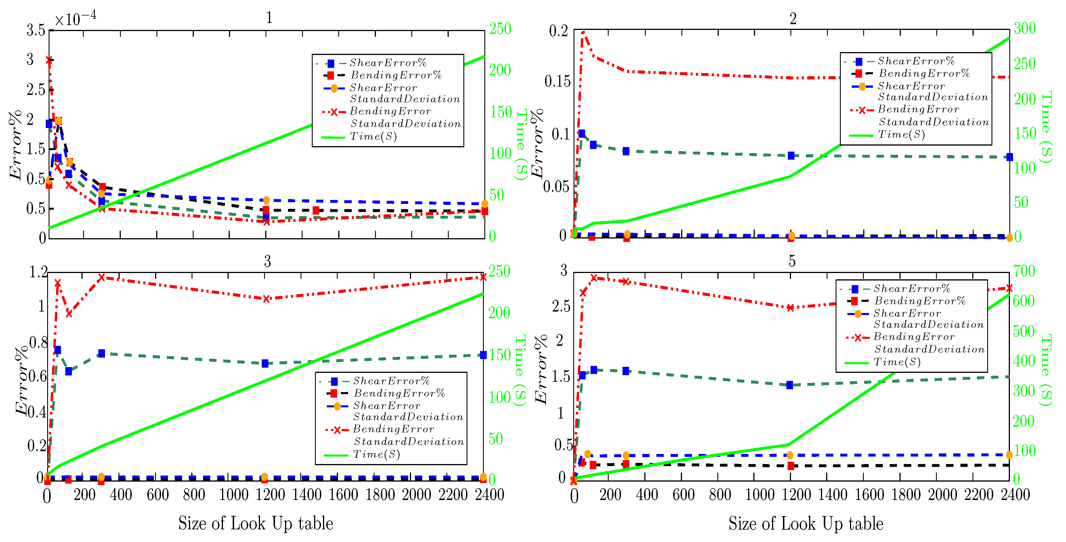
The shear and bending Errors and the Standard deviation results are shown in
Figure 5. Since the
of analysis is an important factor for evaluating the desirability of an operator’s performance, the duration of the process was also measured and documented in these diagrams. In
Figure 5, all analyses with any
reduced the Error by increasing the
, indicating the capability of them in case of suitable size of
Table. The sensitivity of Error to the amount of
, by increasing that reduced. In all of the Errors and standard deviation, disregarding the
, the accuracy is considerably low when the
. Increasing the
increases the analysis
, but the influence of increasing the
on the Errors is not linear. For instance,
has higher accuracy than
. This influence might be related to the value of
and the type of the membership functions. Despite the high probability of low accuracy in using FL in delegating the ACI codes, it can operate more stable (with less scattery results) with suitable adjustment and input.
3.2. Neural Network ()
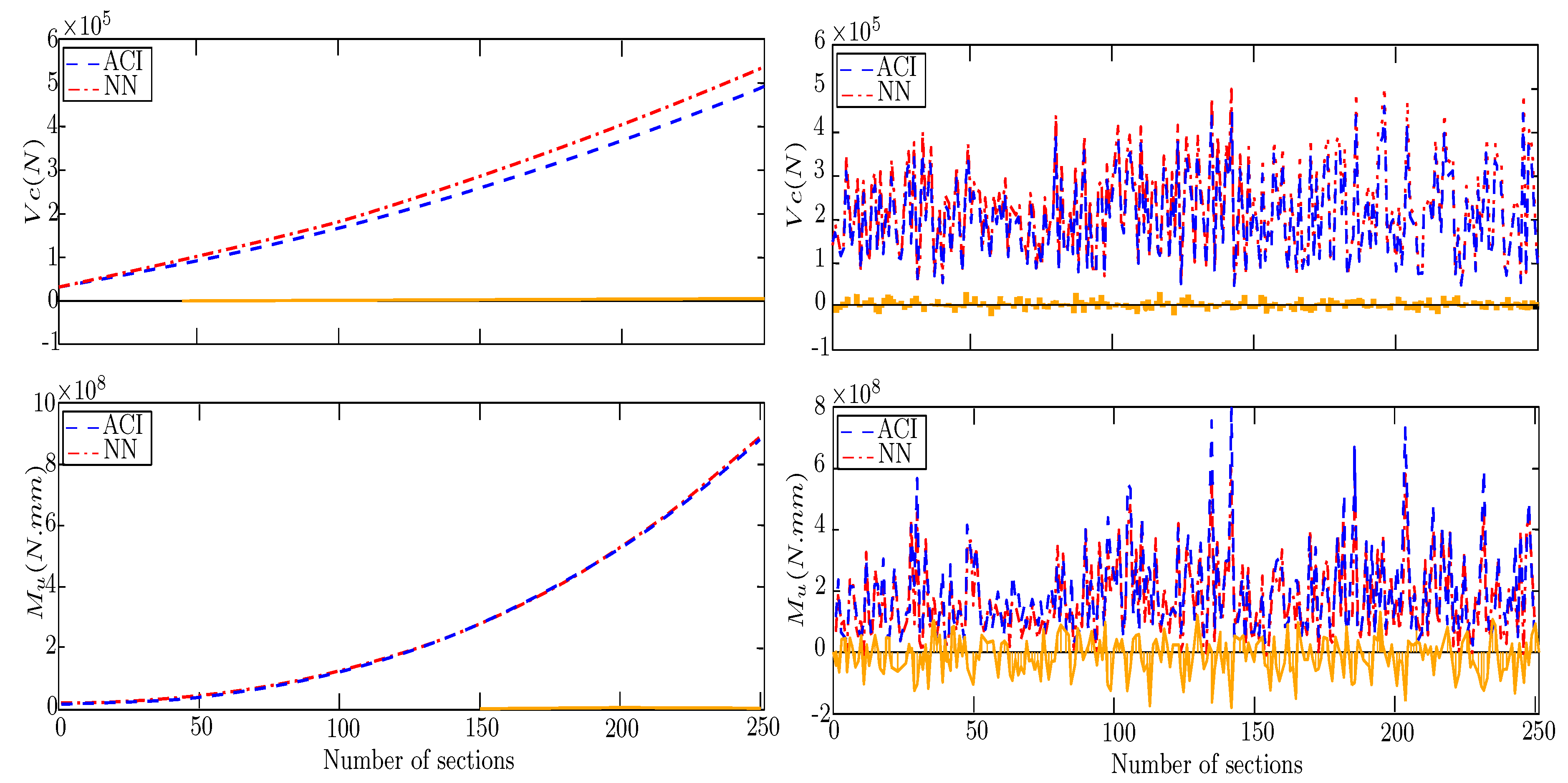
To compare
and FL,
Figure 6 displays the same examples solved and delegated by Neural Network codes. The codes of Neural Networks were developed in MATLAB. In order to fit the Network, as the activation operators, Sigmoid activation (
) and Hyperbolic tangent Sigmoid (
), along with Linear function (
) for transferring the input were selected. In addition to inputs, targets and the number of the hidden layer (NHL), these operators were (by
command) assigned to the Network. For choosing, ’in/out-put’ and ’re/post-processing’ functions were coded. Likewise, operators were coded for removing rows with constant values (
) and mapping rows with minimum and maximum values (
). Furthermore,
for random division of data and every sample (
) was picked, in which
of the data for training and equal percent for validation and tests of the Network selected (
). Additionally, for choosing and helping the train function, Levenberg-Marquardt (
) and Mean squared Error (
) were assigned to the Network performance function. In the codes, the number of the hidden layer (
) as an adjustable parameter was regarded (e.g.
).
The same types of
tables as the input imported by Fuzzy were prepared in this section to be interpreted by
.
Figure 6 illustrates the results of these two examples with sorted and randomized input types. In this example, the size of the Table and parameters’ number are 250 & 3 respectively, (
,
). Likewise, the red and blue diagrams show the
and ACI results, while the differences between
and ACI are shown in the yellow bar. The remarkably higher accuracy of
compared to FL in both delegated results is visible. Generally, bending capacity (
), compared to shear (
), has a higher number of effective parameters, which causes the relation between feature and output to be more nonlinear. The Error results in these two examples show that
can present a more exact bending capacity in sorted inputs. Despite this, randomized input bending diagrams show less exact. The
operator also calculated several other examples based on and in compression to FL; it can be calculated that the capability of the Nural Network for delegating the ACI calculation is considerably higher.
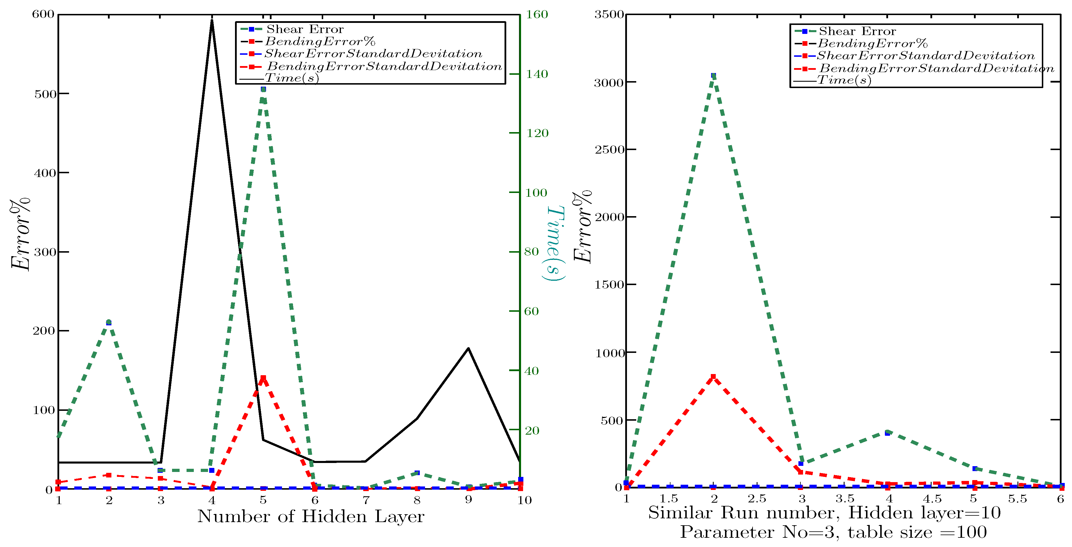
One of the main components of the Nural Network is the number of the hidden layer (NHL). In a series of example same problem (
,
) with different number of hidden layer (
) was repeated,
Figure 7. It can be seen that compared to the chaotic nature of the coded
, the NHL cannot show a strong influence on the results of this example. Based on multiple examples tested by the current study, it can be concluded that increasing the number of layers for more than three layers has more influence on the analysis
than the amount of Errors.
Nonetheless, the main highlight of using
is the chaotic amount of accuracy. In other words, despite the input parameters, in a series of examples were increased gradually, the Error amounts in some were almost zero, and in some, they were several times higher than the maximum amounts of bending and shear capacity. To illustrate, a repetition of the same problem was documented in
Figure 7. In these examples (
,
), the Error of delegating the shear and bending beside the Errors Standard deviation was displayed. It can be seen that the Error in examples
is almost zero while, in example 2, shear is 30, times higher than ACI calculations. Despite FL showing, in general, lower accuracy, such an issue (chaotic results) was not detected. Some examples have acceptable performance in bending Error and are high in shear. Hence, in an operator like
with low robustness, the Error amounts in objects may differ considerably. The high probability of facing low accuracy in the results of FL and, despite high capability, chaotic results of
indicates the necessity of developing a method using the potentials of Fuzzy and
while solving their issues.
It should be remembered that in all MLO in this study against other Multi-Objective optimization algorithms, the objects (here ) are calculated separately in two different parallel interpreting processes.
3.3. Adaptive Neuro-Fuzzy-Inference System (ANFIS)
Adaptive Neuro-Fuzzy Inference System is a hybrid artificial intelligence model that combines the strengths of FL and Neural Networks. This operator was similarly developed in MATLAB, regarding the same feature coded for Fuzzy and . As the , features of the beam section and the capacity of the beams calculated by ACI codes were selected. Inputs by Gaussian membership function and linear output types in layers were selected (). To remove and generate the system, subtractive clustering was chosen (). The options by were assigned to create dialogue box . The data, including the inputs, outputs and training data, were assigned to the , by , selected FIS generation approach. During the initial investigations, with and , both tried and due to this study’s low influence and concentration, were in preparation for the results used. The cluster number was , and the Exponent matric was partitioned to . The number of maximum iterations and the number of Epochs was , and the minimum improvement was ’’. In these studies, the initial step was 0.01 and the step size was 0.9, while 1.1 was the step size increasing rate and 0 as the error target was assigned.
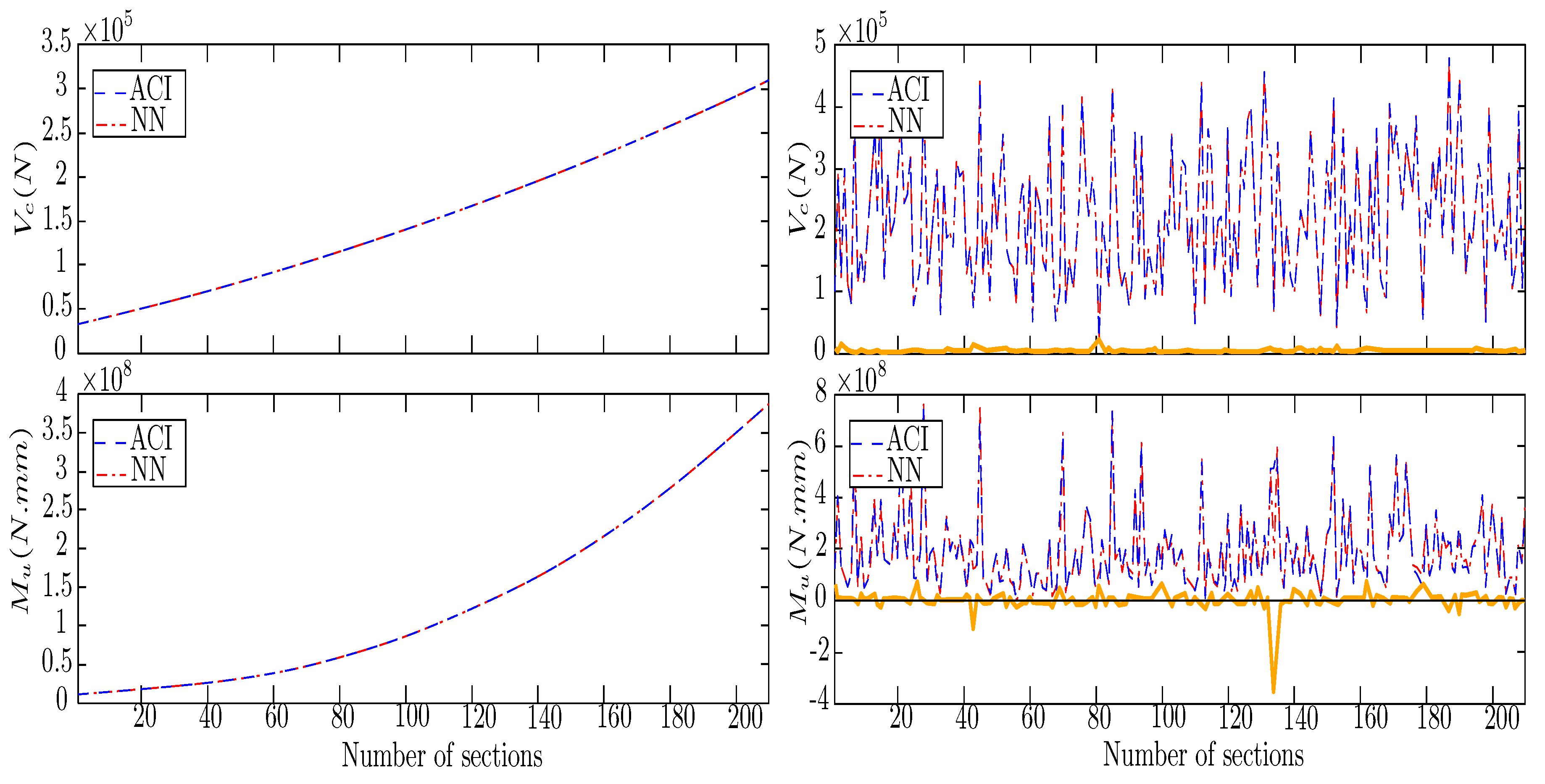
Like the previous section, as the first examples, three parameters and the sorted and randomized inputs were selected to compare directly.
Figure 8 shows the results of ANFIS in the delegation of beam calculations. It can be seen that the Error in the calculation of bending and shear capacities is deficient (approaching zeros). Generally, ANFIS has a robust homogeneous performance. The range of examples made by ANFIS displayed higher accuracy in calculating the bending in all examples with different
and
, was repeated in average the bending Error is less than shear Error. The shear Error increases, especially with a low number of
and
. In this investigation, different example series were solved by ANFIS. Based on an example with
when the number of parameters is 7, the calculation accuracy is
times lower than the same operation with a 1 parameter. Despite this, the Error range in both is less than
and ignorable,
Figure 9.
Similar results were experienced for the Standards deviation . It might be concluded that the capability of this operator is more suitable for complex structural issues. If the duration of the process as the analyzing is regarded, increasing the is the main factor for raising the . Likewise, increasing the , from 1 to 7, when in average increased the analyzing to . ANFIS, in repeating the same problem, had the same results, proving its analytical stability. Additionally, increasing the size of in sorted input type proved its low positive influence on reducing the Error, but randomized input increased the Error.
3.4. Comparison between the Three MLO
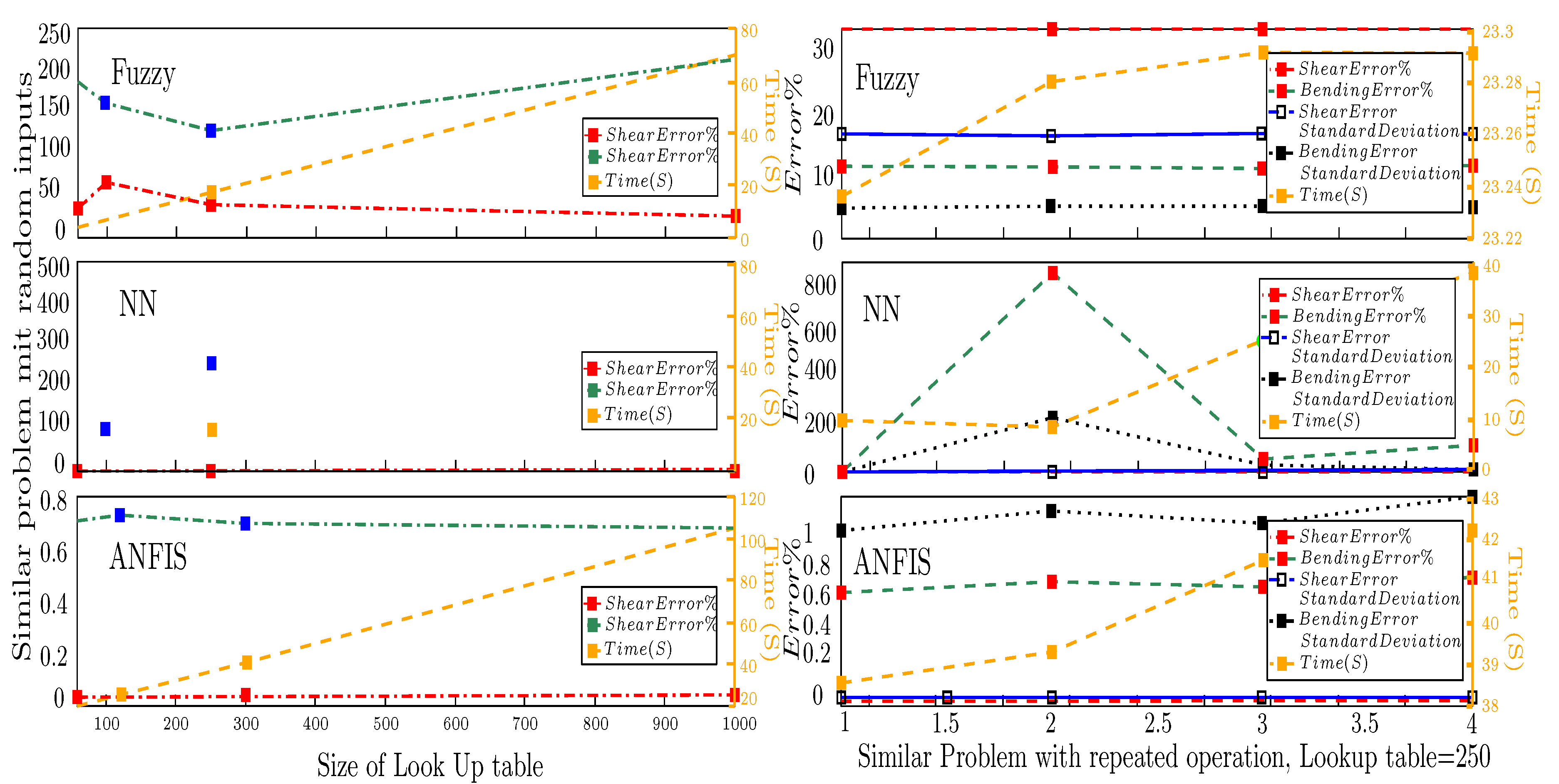
Figure 10 (Left) displays a series of examples based on a randomized
table, in which
range increases up to 1000. The Error of
, in addition to the analyzing duration by increasing the
increases, is entirely visible in
diagrams. ANFIS, in addition to having higher accuracy, has a robust performance; it did not indicate significant changes in
&
capacity representation of the ACI bending and shear capacity with less than
differences. In this range, the analyzing
of Fuzzy and Neural Networks are similar and for the same problems are almost
of ANFIS. The other examples showed higher differences between the
of FL and
compared to ANFIS by increasing the
.
Likewise, the duration of Fuzzy has an exponential relation with
and
. It means that in representing the small problem, FL performs faster than
and ANFIS. As mentioned, this study just selected MATLAB as a proper platform, and rewriting the codes in primary programming languages (e.g.
) can considerably reduce the analyzing
. It should be mentioned that the time for preparing the
table was not considered when discussing the analyzing
. Accuracy (Error), duration (time) and robustness of the operator are the three selected. Hence,
Figure 10 (Right) contrasts the MLO operations’ robustness by running the same problem with times to compare directly.
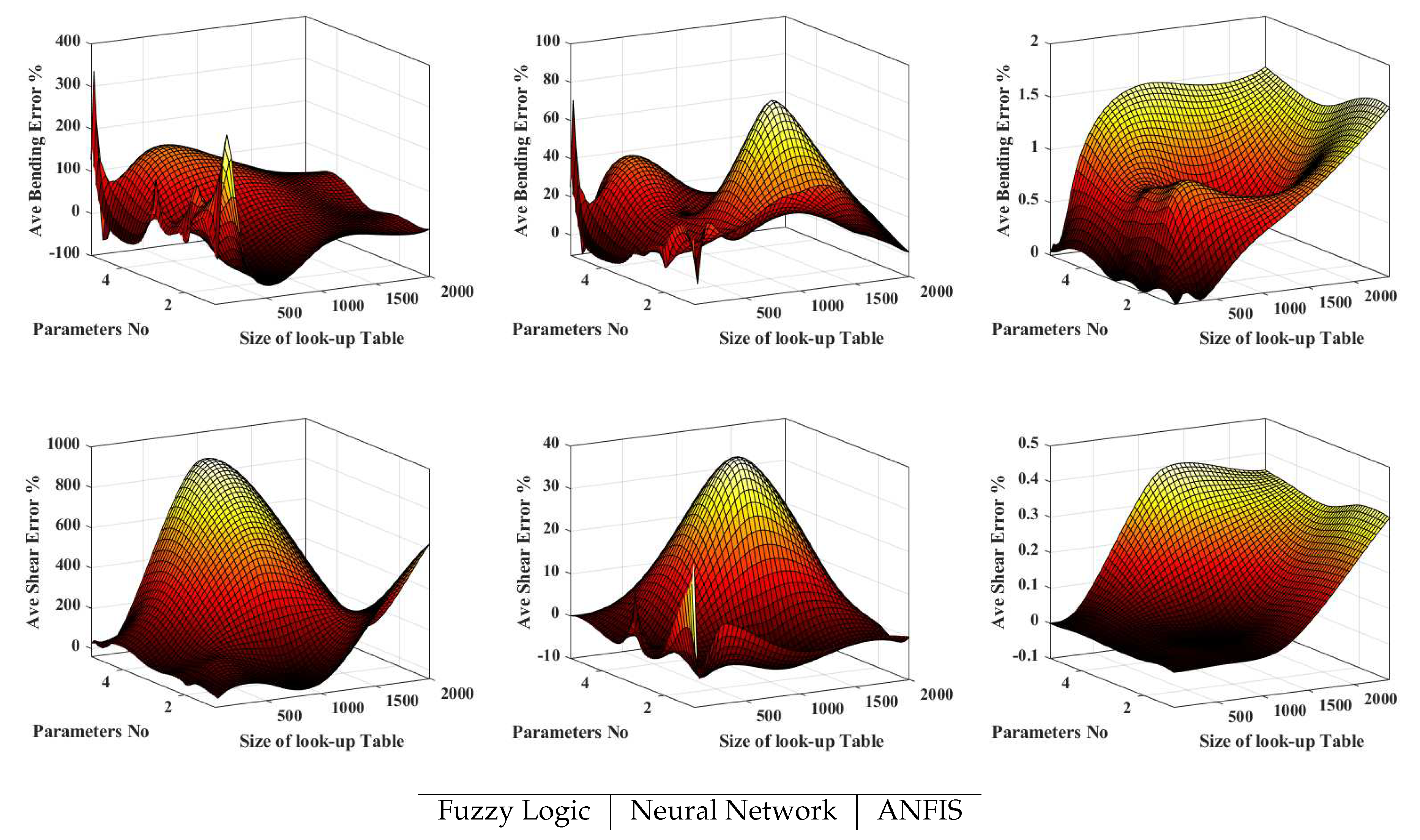
A general contrast between the performance of the MLO was made by fitting 3D surfaces to the results. This surface is also fitting managed in MATLAB, while the size of the
table (
) and parameter Number (
), along with the average amount of shear and bending amounts, were separately selected.
Figure 11 displays the accuracy of all three coded Machine Learning operators (including FL,
and ANFIS). The top diagrams of
Figure 11 illustrate the bending and shear errors in the down row. The results of various analyses were shown next to each other in these diagrams. The average amounts of shear and bending differences (Error between ACI and MLO), regarding the range of
,
, by fitting surfaces on them were plotted in MATLAB. Generally, one of the main usages of the MLO is curve fitting. Despite the higher power of MLO for fitting continuous surfaces to the discrete data and synergy between curve fitting and all discussed MLO, due to simpleness, in this diagram, simple codes in MATLAB were used.
FL has the lowest accuracy despite the highest stability in the calculations and results. The amount of Error in the calculation of the bending capacity gets lower by reducing the size of the Table and increasing the number of parameters. On average, the bending calculated by FL and ACI in this range maximum differ , while for shear, this difference increases to . Generally, FL initial coding starts with defining the Linguistic Variables. Linguistic Variables include 1- The name of the variable (e.g. ), 2- Amount of variables for each group (e.g. in [0.2,0.5,0]), 3- Range of the changes in variables (e.g. Height of a beam), and 4-Fuzzy set. Hence, each Linguistic Variable can be defined. It enables the FL to convert the initial digits to Fuzzy parameters (called Fuzzification) and, after the operation, to digits (called Defuzzification). This will be continued by developing the Rules for the logical implications needed. The conversion of the digits to logical and Linguistic variables enables the FL to import different types of data (e.g. Verbal information of a questionary form) but can be the reason for reducing the accuracy of the results (increasing the Error).
The results of on the average show () Error for shear and bending, respectively, which is considerably lower than FL. Likewise, increasing the size of the Table or, in other words, preparation of more initial data (e.g. from numerical or experimental structural analyses) can reduce the Error and scattered results faced more in calculating bending capacities.
Due to the issues of FL and
(i.e. low accuracy and analyzing stability), this study also developed ANFIS codes. The results of this operator, which has the advantages of FL and
, are shown in the last column of
Figure 11. Against FL and
, enlarging the
table can considerably increase the analysis
and does not enhance the accuracy. Increasing the number of parameters (beams sections feature) also reduces accuracy. Additionally, its performance in the calculation of shear compared to bending calculation is more accurate. ANFIS, with all sizes of inputs, should have entirely acceptable performance while, on average, the differences between the ACI direct calculation and ANFIS for bending and shear are (
). The maximum experienced average Error, in general, is less than
, which indicates the capability of ANFIS for delegating standard designs.
Figure 1.
Section’s Calculation Chart.
Figure 1.
Section’s Calculation Chart.
Figure 2.
Random features of the 50 beam sections and the capacity based on ACI.
Figure 2.
Random features of the 50 beam sections and the capacity based on ACI.
Figure 3.
Results of Fuzzy operation with 250, table size and three variables and ’gaussmf’.
Figure 3.
Results of Fuzzy operation with 250, table size and three variables and ’gaussmf’.
Figure 4.
Results of Fuzzy operation with ’250’, table size and ’3’ variables and ’gaussmf’.
Figure 4.
Results of Fuzzy operation with ’250’, table size and ’3’ variables and ’gaussmf’.
Figure 5.
Results of parametric adjustment of Fuzzy operator, .
Figure 5.
Results of parametric adjustment of Fuzzy operator, .
Figure 6.
Neural Network Results of sorted (left) and randomize (right) inputs, ,.
Figure 6.
Neural Network Results of sorted (left) and randomize (right) inputs, ,.
Figure 7.
Neural Network Results, for (right) discussing the influence of NHL and (left) robustness of the results in repetition of an exact problem.
Figure 7.
Neural Network Results, for (right) discussing the influence of NHL and (left) robustness of the results in repetition of an exact problem.
Figure 8.
ANFIS results of sorted (left) and randomize (right) inputs, ,
Figure 8.
ANFIS results of sorted (left) and randomize (right) inputs, ,
Figure 9.
Performance of ANFIS ,.
Figure 9.
Performance of ANFIS ,.
Figure 10.
Time comparison as the for regarding different MLO, number of parameters and size of the table, without the duration of time needed for the production of the table and stability of the results on repetition of the similar problems.
Figure 10.
Time comparison as the for regarding different MLO, number of parameters and size of the table, without the duration of time needed for the production of the table and stability of the results on repetition of the similar problems.
Figure 11.
Comparison between the performances of the discussed MLO, by fitting surfaces to shear and bending Errors, while , as the parameter ranges were regarded.
Figure 11.
Comparison between the performances of the discussed MLO, by fitting surfaces to shear and bending Errors, while , as the parameter ranges were regarded.
Table 1.
Verification of the accuracy of the coded beam calculations in comparison to the references.
Table 1.
Verification of the accuracy of the coded beam calculations in comparison to the references.
|
He |
Wi |
fc |
fy |
As’ |
As |
St |
Perf |
|
Mu |
Vu |
Ref |
| No |
mm |
mm |
N/ |
N/ |
|
|
mm |
name |
mm |
N.mm |
N |
Name |
Amount |
| 1 |
500 |
350 |
30 |
400 |
942 |
4825 |
- |
2.1.2 |
174-174 |
7.1e08 |
- |
11-5 [26] |
Mu:7.1e08 |
| 2 |
300 |
350 |
21 |
400 |
942 |
3217 |
- |
1.1.2 |
149-145 |
2.1e08 |
- |
12-5 [26] |
Mu:1.9e08 |
| 3 |
500 |
400 |
35 |
400 |
- |
1357 |
- |
3.2.1 |
47 |
2.6e08 |
- |
5-5 [26] |
Mu:2.4e08 |
| 4 |
350 |
200 |
32 |
500 |
- |
804.2 |
|
3.2.1 |
75-74 |
1.3e08 |
- |
[27] |
Mu:1.2e08 |
| 5 |
3500 |
2000 |
32 |
500 |
- |
8040 |
- |
3.2.1 |
75-74 |
1.4e10 |
- |
[27] |
Mu:1.4e10 |
| 6 |
500 |
300 |
35 |
400 |
- |
- |
10@80 |
- |
- |
- |
3.53e05 |
1-7 [1] |
Vu:3.5e05 |
| 7 |
520 |
350 |
21 |
300 |
- |
- |
12@125 |
- |
- |
- |
2.92e05 |
3-7 [26] |
Vu:2.8e05 |
| 8 |
500 |
300 |
30 |
400 |
1231 |
2412 |
- |
2.2.1 |
72 |
- |
3.95e8 |
3-8 [28] |
Mu:3.9e08 |
| 9 |
500 |
450 |
25 |
400 |
- |
- |
12@100 |
- |
- |
- |
3.97e05 |
[29] |
Vu:4.1e05 |
| 10 |
650 |
300 |
21 |
275 |
- |
3220 |
|
3.1.1 |
|
5.0e08 |
|
[27] |
Mu:4.8e08 |
Table 2.
Selected Range of Changes in the Variables.
Table 2.
Selected Range of Changes in the Variables.
|
|
|
|
|
|
|
|
| No |
mm |
mm |
|
|
|
|
mm |
| Range |
[150-1000] |
[100-300] |
[20-70] |
[200-600] |
[0-393] |
[158-1570] |
[500-50] |
Table 3.
Influence of parameters changes on the beam capacities (all numbers are percentages).
Table 3.
Influence of parameters changes on the beam capacities (all numbers are percentages).
| No |
|
|
|
|
|
|
|
|
|
| 1. |
2,00 |
2,00 |
2,00 |
2,00 |
2,00 |
2,00 |
2,00 |
8,15 |
7,18 |
| 2. |
2,00 |
2,00 |
2,00 |
2,00 |
2,00 |
2,00 |
1,00 |
8,15 |
4,74 |
| 3. |
2,00 |
1,00 |
1,00 |
1,00 |
1,00 |
1,00 |
1,00 |
2.03 |
2,07 |
| 4. |
1,00 |
2,00 |
1,00 |
1,00 |
1,00 |
1,00 |
1,00 |
1,08 |
1,32 |
| 5. |
1,00 |
1,00 |
2,00 |
1,00 |
1,00 |
1,00 |
1,00 |
1,07 |
1,14 |
| 6. |
1,00 |
1,00 |
1,00 |
2,00 |
1,00 |
1,00 |
1,00 |
1,95 |
1,54 |
| 7. |
1,00 |
1,00 |
1,00 |
1,00 |
2,00 |
1,00 |
1,00 |
1,00 |
1,00 |
| 8. |
1,00 |
1,00 |
1,00 |
1,00 |
1,00 |
2,00 |
1,00 |
1,95 |
1,00 |
| 9. |
1,00 |
1,00 |
1,00 |
1,00 |
1,00 |
1,00 |
1,00 |
1,00 |
1,00 |
