Exploring Effectiveness and Usability of Synthetic Sar Data in Real Classification Scenarios: A Case Study

In recent years, Synthetic Aperture Radar (SAR) has received attention in the Automatic Target Recognition (ATR) field due to its ability to acquire images both day and night, combined with the superior resolution offered by the latest sensors. However, despite advances, there remains a deficiency in dataset quality and quantity. This has necessitated the use of simulated data to overcome challenges associated with obtaining large quantities of high-quality images of targets and their subsequent labeling. In this study, we trained a Convolutional Neural Network (CNN) using a simulated dataset, subsequently employing it to classify real images from the MSTAR dataset. Traditional training methodologies often struggle with generalization when confronted with domain disparities between simulated and real data. To mitigate this, we exploited Margin Disparity Discrepancy (MDD), a domain adaptation technique not previously explored in SAR context. Findings from this study showcased a 13% increase in classification accuracy and improved generalization using MDD. Through Explainable AI (XAI) techniques such as t-SNE and other metrics like Kullback Leibler Divergence (KLD), we revealed a more distinct alignment of feature spaces between the two domains after domain adaptation, emphasizing MDD’s role in enhancing model accuracy and generalization.

Keywords:

Subject: Engineering - Telecommunications

1. Introduction

Synthetic Aperture Radar (SAR) has become an influential remote sensing technology for Earth observation, enabling the capture of high-resolution images regardless of weather conditions or daylight availability. In recent years, the advancement in image quality and resolution has opened doors for the successful application of Artificial Intelligence (AI) in various tasks, such as object detection[1,2,3], object classification[4,5,6,7], image colorization [8,9], change detection[10,11,12] and noise reduction[13,14,15].

Despite the progress made, the practical implementation of SAR-based applications in real-world scenarios still faces a significant challenge due to the lack of extensive and reliable training datasets as reported also in [16,17]. Although the sources for acquiring high-resolution imagery are increasing and new data is becoming publicly available, the process of labeling SAR images remains a major obstacle. While for certain applications like Ship Detection, the utilization of AIS data can offer a reliable source for annotating a large number of images in an automated way[18,19], it is not feasible for most other targets of interest, including vehicles, airplanes and military objects. Additionally, data augmentation techniques are limited in this domain due to the complex interplay between acquisition geometry and backscatter values, which cannot be replicated by simple scene rotations as in Electro-Optical (EO) imagery.

One potential solution to address the aforementioned challenges lies in the utilization of SAR simulators [20]. These software tools enable, given the 3D CAD models of the targets, the generation of a vast volume of labeled data by leveraging various permutations of sensor parameters, target positioning, and angles of sight. SAR simulators offer the flexibility to create diverse synthetic datasets, mimicking real-world scenarios and providing valuable training resources.

In this paper, we present a comprehensive analysis aimed at assessing the effectiveness and usability of a Convolutional Neural Network (CNN) based classifier across simulated and real domains for SAR imagery. We ultimately suggest an approach to boost the performances of the CNN using Margin Disparity Discrepancy (MDD), an Unsupervised Domain Adaptation (UDA) technique originally introduced by Zhang et al. [21], which enhance the CNN classifier’s ability to extract domain invariant features. This enhancement ultimately leads to improved generalization and overall performance. Obtained results are validated through an in-depth analysis, which validate the capacity of DA in bridging from simulated to real domain in SAR context.

Previous researchers employed different methods to address the discrepancies between simulated and real domains in SAR imagery. One such method is domain randomization [22], which promotes a robust classifier trained on synthetic data. However, this method requires a vast amount of additional simulations for better model generalization, an aspect that can be problematic in terms of space and computational requirements. The concept of transfer learning has also been utilized effectively for improving classification accuracy in the aforementioned context [23,24]. While this technique can improve the model performances it requires labelled data in the real domain, which can be hard or nearly impossible to obtain in many situations. Another novel approach involves the hierarchical combination of a Convolutional Neural Network (CNN) and image similarity measures to handle the distribution differences between simulated and real data [25]. This approach focuses on identifying and reclassifying the ’hard samples’ that are prone to misclassification, thus enhancing the performance of the recognition methods. However, this approach may face challenges with the misclassification of hard samples, reliance on similarity measures in high-dimensional spaces, and the complexity of the bagging ensemble technique.

Our employed method emphasizes the quality of simulation over quantity, effectively delegating the task of domain generalization to the neural network’s architecture. By using a Domain Adversarial Neural Network (DANN) framework for Domain Adaptation (DA) as previously demonstrated by [26], and integrating it with an MDD-based loss function, we concurrently achieve object classification and extraction of domain invariant features. This approach also proves to be computationally efficient during the inference phase. Specifically, the neural network (NN) branch responsible for domain discrimination is discarded after training. Consequently, the final classifier solely consists of the initial CNN architecture, which results in a significant reduction in computational overhead.

2. Materials and Methods

A core aspect of our research lies in the construction of a unique simulated dataset obtained with the usage of a path tracing based SAR simulator. This chapter details the material utilized, the pre-processing steps, and the methods employed for executing this research.

2.1. Simulated Dataset

The simulated dataset was derived using a proprietary SAR simulator calibrated on the parameters of the Moving and Stationary Target Acquisition and Recognition (MSTAR) dataset [27]. Our decision to leverage the MSTAR dataset as a simulation reference is rooted in its diverse collection of images featuring various targets against a simplistic background, captured from multiple angles. This aspect holds significant relevance in SAR imagery, where even slight deviations in object orientation can result in substantial disparities in radar signatures. With our research being fundamentally aimed at the real-world application of ATR, we specifically selected samples acquired at a depression angle of 45°. This angle typically provides an optimal balance between spatial resolution and sensitivity to topographic variations. This selection criterion restricted the number of viable classes in MSTAR to three: ZSU-23, BRDM2 and 2S1. We generated 360 simulated images for each class at every integer degree of rotation, resulting in a total of 1080 data samples. The simulation parameters, summarized in Table 1, were derived from the original file header provided by MSTAR, with the exception of the thermal noise parameter, which we estimated directly from the data.

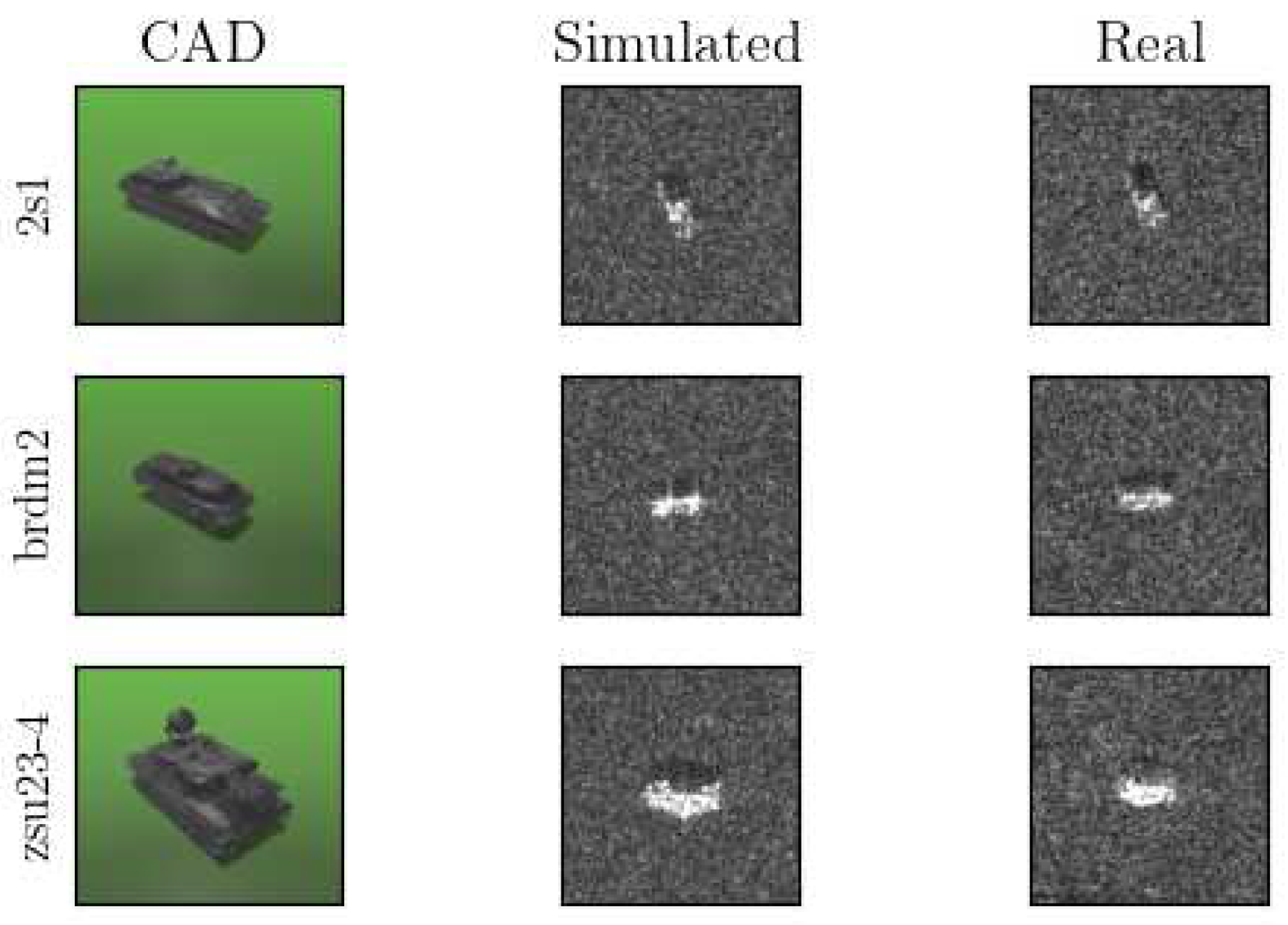
The 3D CAD models employed in the simulation phase were sourced from public online databases. These models may not perfectly replicate the original objects, leading to an approximation in the computed radar signatures. This approximation could potentially influence the classifier’s performance, yielding sub-optimal results. Thus, such limitations should be carefully considered in real-world applications. For effective simulation, the 3D model requires parametrization through the assignment of physical materials to each constituent surface. In our approach, we approximated the entire object with a metallic surface thereby obtaining an ideal scatterer. However, it is important to note that the original MSTAR images display a significant amount of rust on tank surfaces. This detail might result in a slightly different interaction with SAR microwaves, something not fully captured in our simulation due to our previous assumption on the material. In Figure 1 is shown a comparison between MSTAR images and simulated ones.

In subsequent sections, we use the term "real" to refer to the MSTAR data meanwhile our generated data is referred to as "simulated".

2.2. MSTAR Dataset

As a benchmark for our simulations and a test set for our classifier, we used the previously mentioned MSTAR dataset. Produced by the U.S. Army’s National Ground Intelligence Center, MSTAR is a publicly accessible SAR dataset featuring high-resolution images of military targets captured under various conditions, orientations, and depression angles from an airborne platform. As previously validated by researchers in [22], this dataset serves as a principal resource for SAR-based Automatic Target Recognition (ATR) studies.

2.3. Data Preprocessing

Before feeding SAR images to our classifiers, we performed some preprocessing steps to ensure data compatibility with our neural network and optimal feature extraction. With an aim to retain the maximum amount of relevant information while enhancing object features and mitigating background contribution, we employed a quarter-power magnitude stretch. This technique, derived from Doerry [28], allows compressing the high dynamic range of SAR imagery into a smaller fixed range, in our case between 0 and 255. The specific formula utilized to stretch the images is as follows, where "image" denotes the amplitude value of the original complex data:

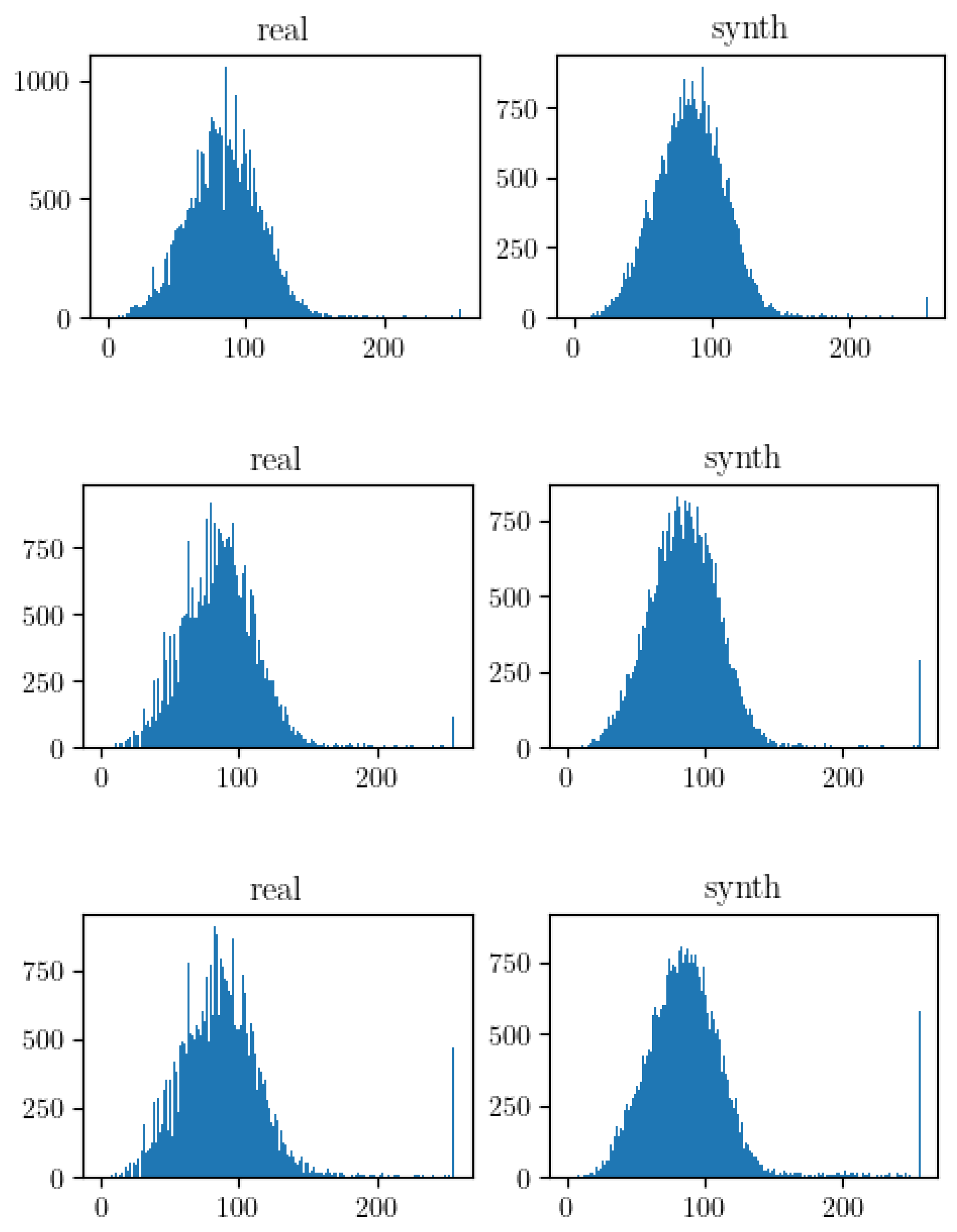
clip (255 \cdot \frac{\sqrt{image}}{3 \cdot median (\sqrt{image})}, 0, 255)

(1)

This procedures ensures that the input data is appropriately formatted and normalized, facilitating effective learning by the neural network. In Figure 2 the histograms of the six images used in Figure 1 are shown.

2.4. Domain Adaptation

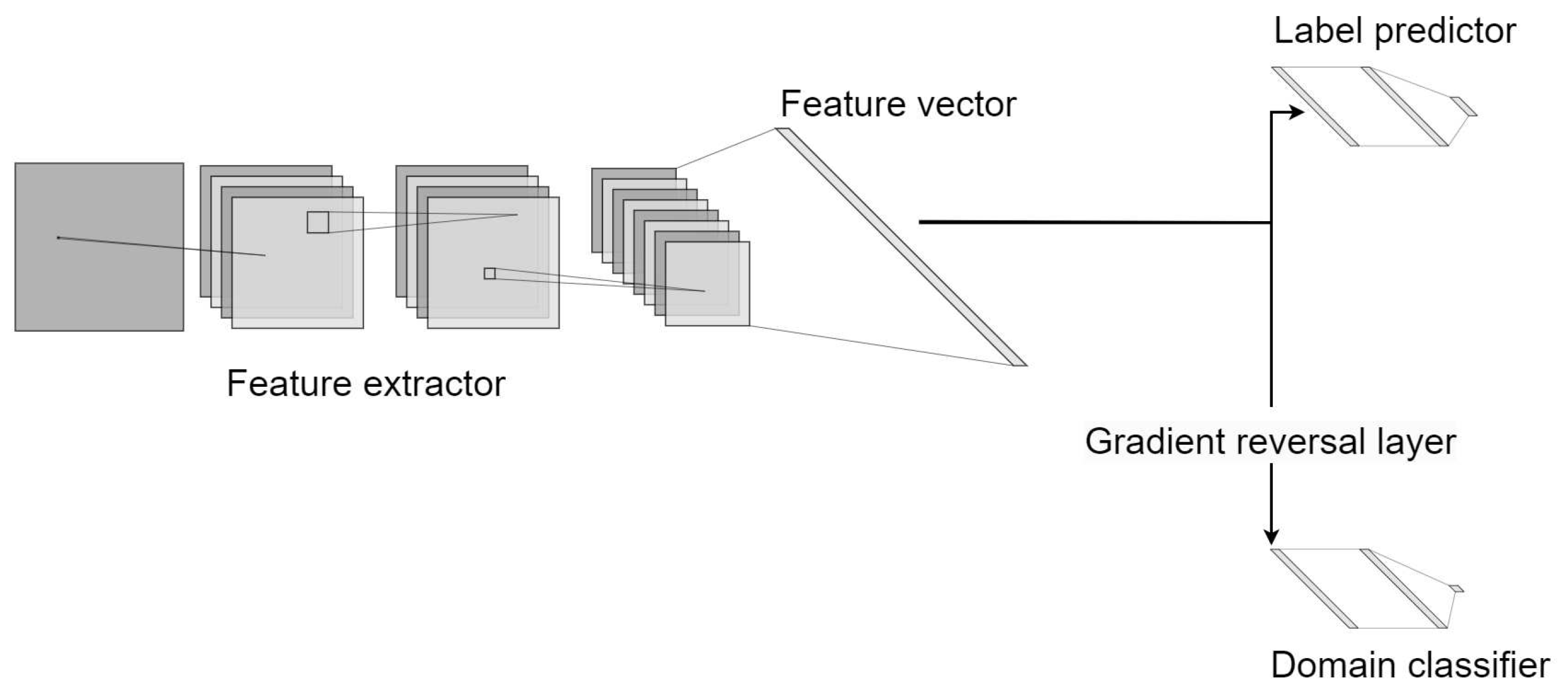
The core of this research lies in the application of an unsupervised domain adaptation technique to extract domain-invariant features. The method we used is margin disparity discrepancy, a technique designed by Zhang [21] that minimize the distribution disparity between source (in our case, simulated) and target (real) domains. Domain-invariant features are very important in real case scenario, a model that is independent from the original domain is expected to generalize better and give stable performances across different use-cases. The core of this technique lies in the application of a DANN where one branch performs multi class classification and the other tries to distinguish the domain from which an image is coming. As demonstrated theoretically by the authors, the expected error to be minimised during the training procedure is bounded by the sum of four different components: the empirical margin error on the source domain, the empirical MDD (Margin Disparity Discrepancy) which we want to minimize, the ideal error and some complexity terms, the last two of which are a function of context parameters and therefore cannot be minimised by the training procedure. Intuitively, the MDD function is a way to measure the difference of distributions between to different domains formulated as the difference between the expected risks of source and target examples within a margin. The main idea is that by minimizing this loss composed by the sum of the standard classifcation loss and the MDD loss, the NN learns to correctly classify source examples while reducing the margin for target examples. This way, MDD encourages the classifier to generate a decision boundary that not only correctly classifies source data but also lies close to the target data, thereby bridging the gap between the two domains. The architecture of our CNN is summarized in Figure 3. A DANN can be seen as three separated networks, a feature extractor, a label predictor, and a domain classifier. For feature extraction we employ a ResNet-50 model leveraging the pre-existing knowledge encapsulated within the ImageNet weights, the initial blocks of the ResNet-50 model are frozen, with only the final block being fine-tuned during the training phase. The label predictor and the domain classifier follow a rather straightforward design, adopting a Fully Connected Network (FCN) architecture of two layers with a dropout layer in the middle. Notably, the domain classifier branch incorporates a Gradient Reversal Layer (GRL). The GRL is a crucial component of the DANN, this layer does not alter the forward pass, and thus, the input passed through this layer remains unchanged. However, during the backward pass, GRL negates the gradient, essentially reversing the direction of the gradient during backpropagation. Mathematically, if x is the input to the GRL and y the output, the forward and backward operations can be represented as:

\begin{matrix} y & = x, \\ \frac{d y}{d x} & = - λ, \end{matrix}

The variable

λ

in these equations is a hyperparameter that regulates the degree of gradient reversal, thereby controlling the trade-off between minimizing the discrepancy across domains (source and target) and maximizing the task-specific classification loss. This balance enables the model to simultaneously learn domain-invariant features and perform accurate classification. The hyperparameter

λ

generally ranges between 0 and 1, with the specific value typically being determined through empirical optimization. This reversal of gradients during backpropagation encourages the feature extractor to learn features that can fool the domain classifier, promoting the extraction of domain-invariant features, which ultimately bridges the gap between the source and target domains. This ensures the network learns features that not only maximize the error of the domain classifier but also make it challenging for the domain classifier to distinguish between source and target domains, thereby promoting domain invariance.

2.5. AI Decisions Interpretation

The opaque nature of AI models often results in a perception of these models as ’black-box’ systems, given the complexity involved in understanding the meaning behind their decisions. In order to analyze our results and better comprehend them we employed a few techniques aligned with Explainable Artificial Intelligence (XAI). Our first method of choice was t-distributed Stochastic Neighbor Embedding (t-SNE) [29], a technique particularly suited for the visualization of high-dimensional data,in our scenario, the features extracted by our CNN model. Visualization of clusters formed by t-SNE provides insights into the distinguishing features learned by the model and how different classes and instances separates in the internal feature space. By comparing the features extracted from both the source and the target domains we were able to visually assess the efficacy of DA.

To accurately represent the operative real-world scenario where target labels are unavailable, we also incorporated a Kullback-Leibler Divergence (KLD) analysis on the t-SNE visualizations produced in the real domain. Operating under the assumption that an ideal classifier should generate compact and well-delineated clusters, the application of KL divergence analysis provides a measure of the model’s performance. This analysis enables an evaluation of our model in an entirely unsupervised manner, an approach that better reflects real-world situations.

3. Results

We generated results using diverse configurations within the training pipeline. The following sections detail each step undertaken, and every test is validated with evidence of result quality through the application of the previously mentioned XAI techniques.

3.1. Training without Domain Adaptation

Initially, we established a baseline for our classifier and dataset by fine-tuning a ResNet50 model exclusively using simulated images, and subsequently evaluated its performance on the MSTAR dataset. The insights derived from this experiment are crucial to gauge the inherent capabilities of our classifier and training dataset. The training parameters are shown in the below Table 2.

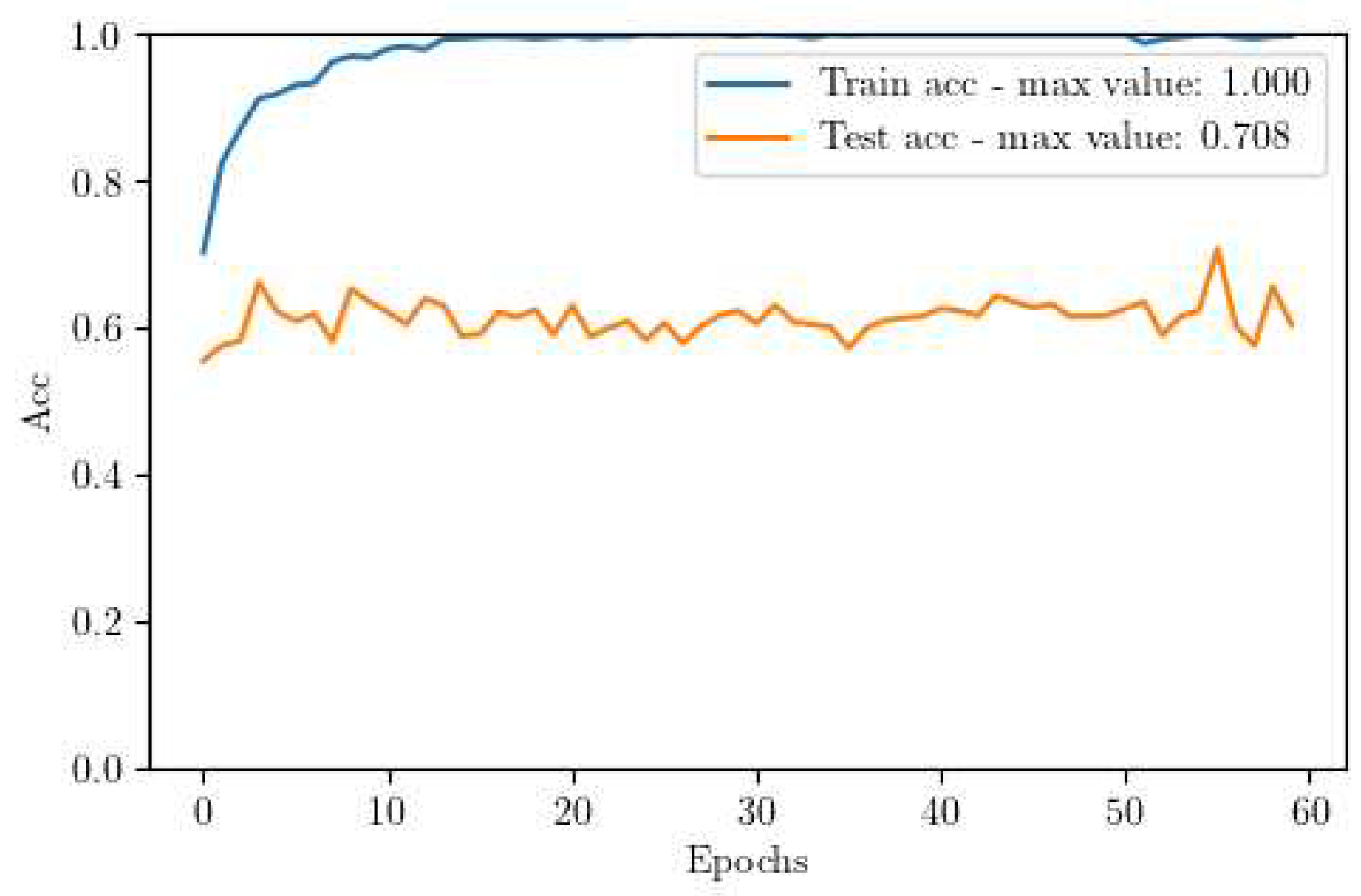
The results acquired from this experiment are displayed in Figure 4. It is evident that the performance is not satisfactory. While the training set swiftly reaches almost 100% accuracy, the test set comprising real images plateaus at approximately 70% accuracy. This gap indicates a significant degree of overfitting to the simulated images and underperformance on real-world data.

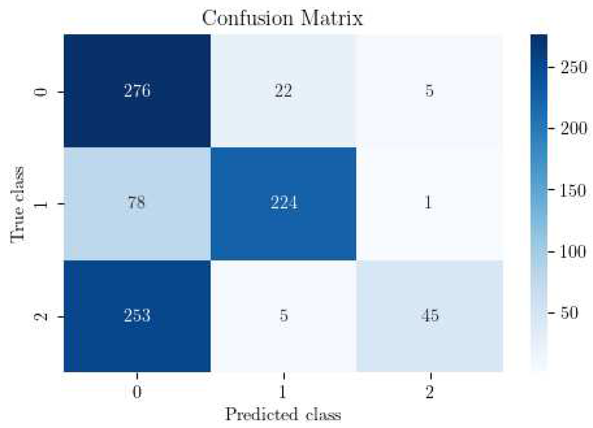
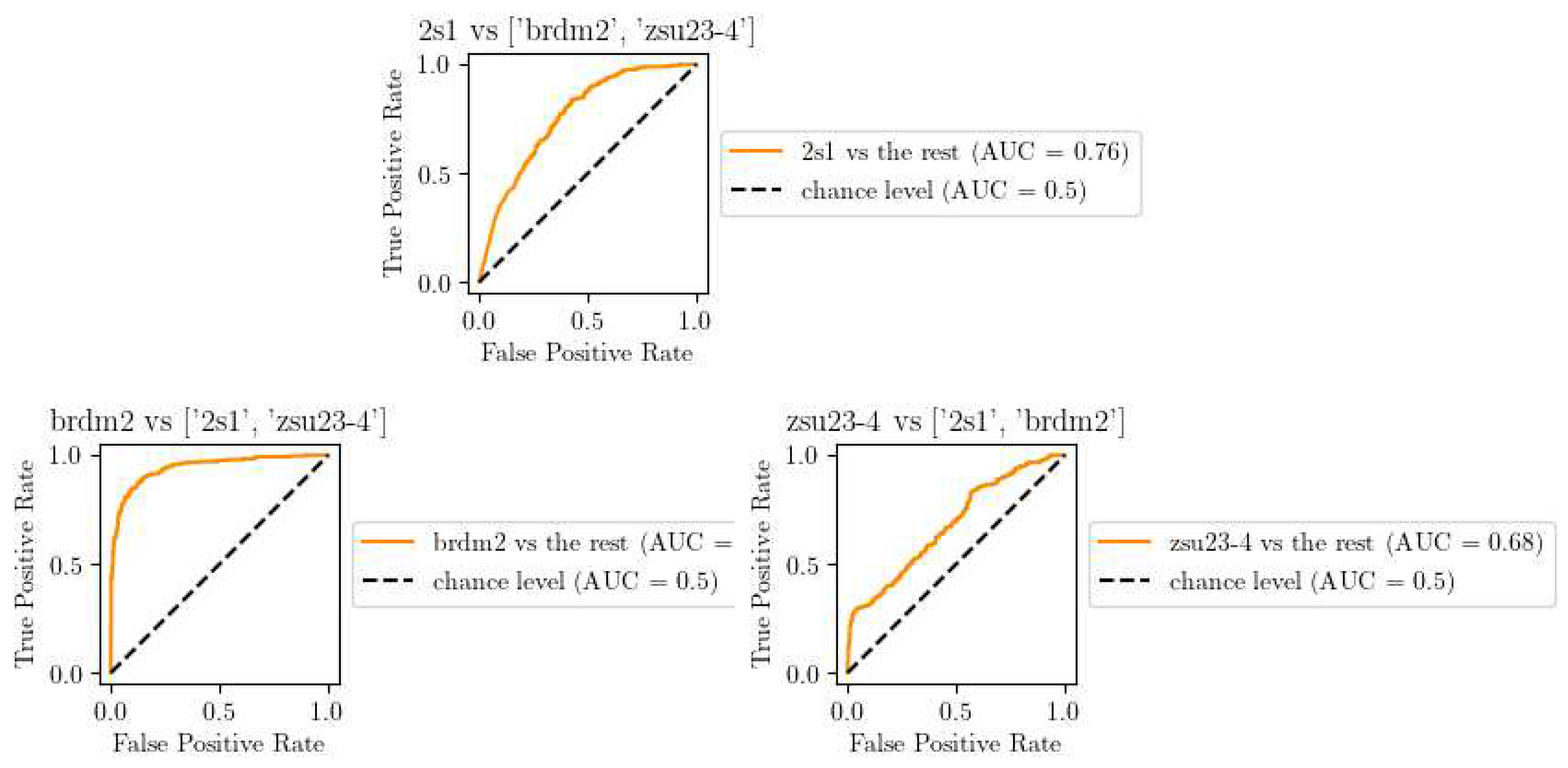
In Figure 5 and Figure 6, it’s noteworthy that our trained model demonstrates significant underperformance, particularly with respect to class 2 (ZSU-23). It misclassifies nearly all instances of this class as class 0, indicating a substantial issue with class-specific accuracy.

3.2. Training with Domain Adaptation

In the DA training pipeline, we integrated MDD using Awesome Domain Adaptation Python Toolbox (ADAPT) python library [30]. We leveraged the architecture shown earlier in Figure 3. The training configuration details are summarized in Table 3.

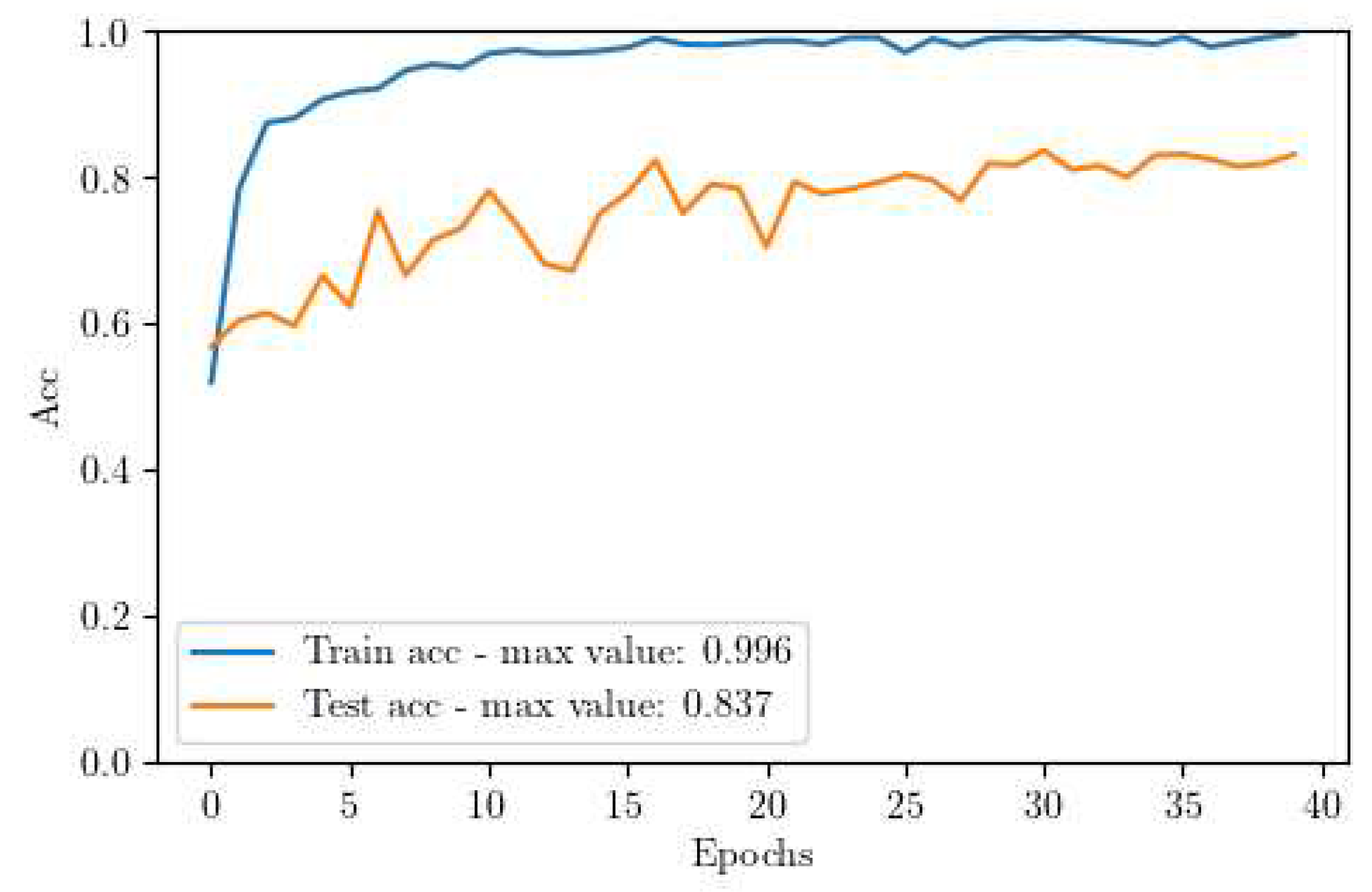
The outcomes of the DA training pipeline are presented in Figure 7. We observed a significant performance boost of approximately 13%, with a steadily climbing training curve that rises from 60% to a peak of 83.7%. This steady increase can be attributed to the varying value of the MDD Lambda, which starts at 0 and increases at each epoch until it reaches 1. This parameter modulates the balance between the classification task and the domain adaptation task. As a result, it prioritizes the classification task at the beginning and gradually shifts focus to domain invariance as the training progresses.

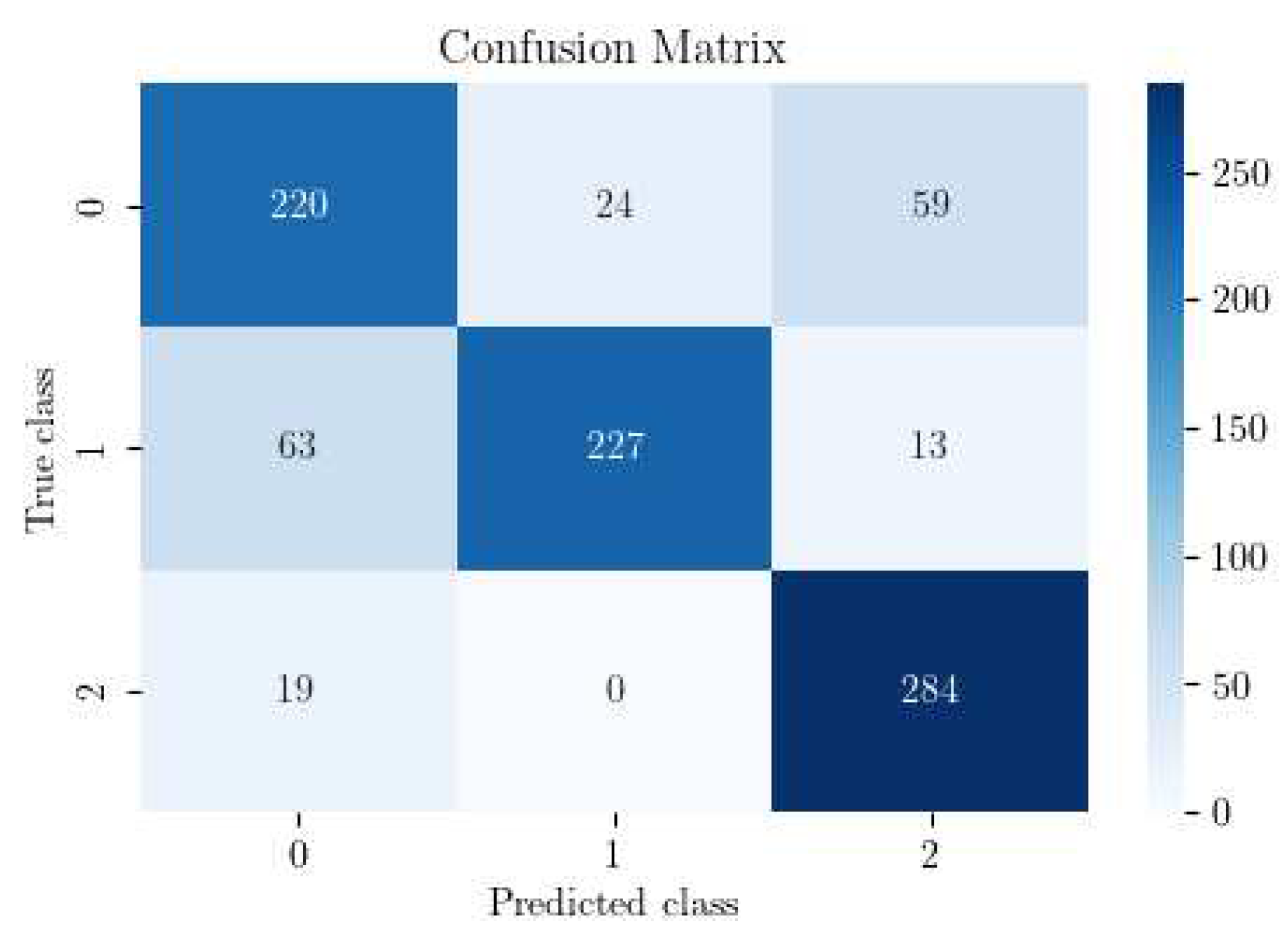
Furthermore, the issue with Class 3 being misclassified entirely is effectively addressed as evidenced in Figure 8 and Figure 9. However, an increased number of instances from Class 0 are now erroneously classified as Class 2.

4. Discussion

The study reveals significant improvements in classifier performance, achieved with only minimal computational overhead. This efficiency extends to practical applications where, during the inference phase, the neural network’s domain-discriminative branch can be excluded. The remaining architecture, identical to the model before DA procedure, retains enhanced capabilities and produces features that are invariant across real and simulated domains. This finding not only aligns with and reinforces existing research on domain adaptation, demonstrating the efficacy of DA techniques in addressing domain discrepancies, but it also pioneers the application of these techniques in a complex domain previously unexplored. This significant extension of DA application showcases the adaptability and potential of such techniques in diverse and challenging contexts.

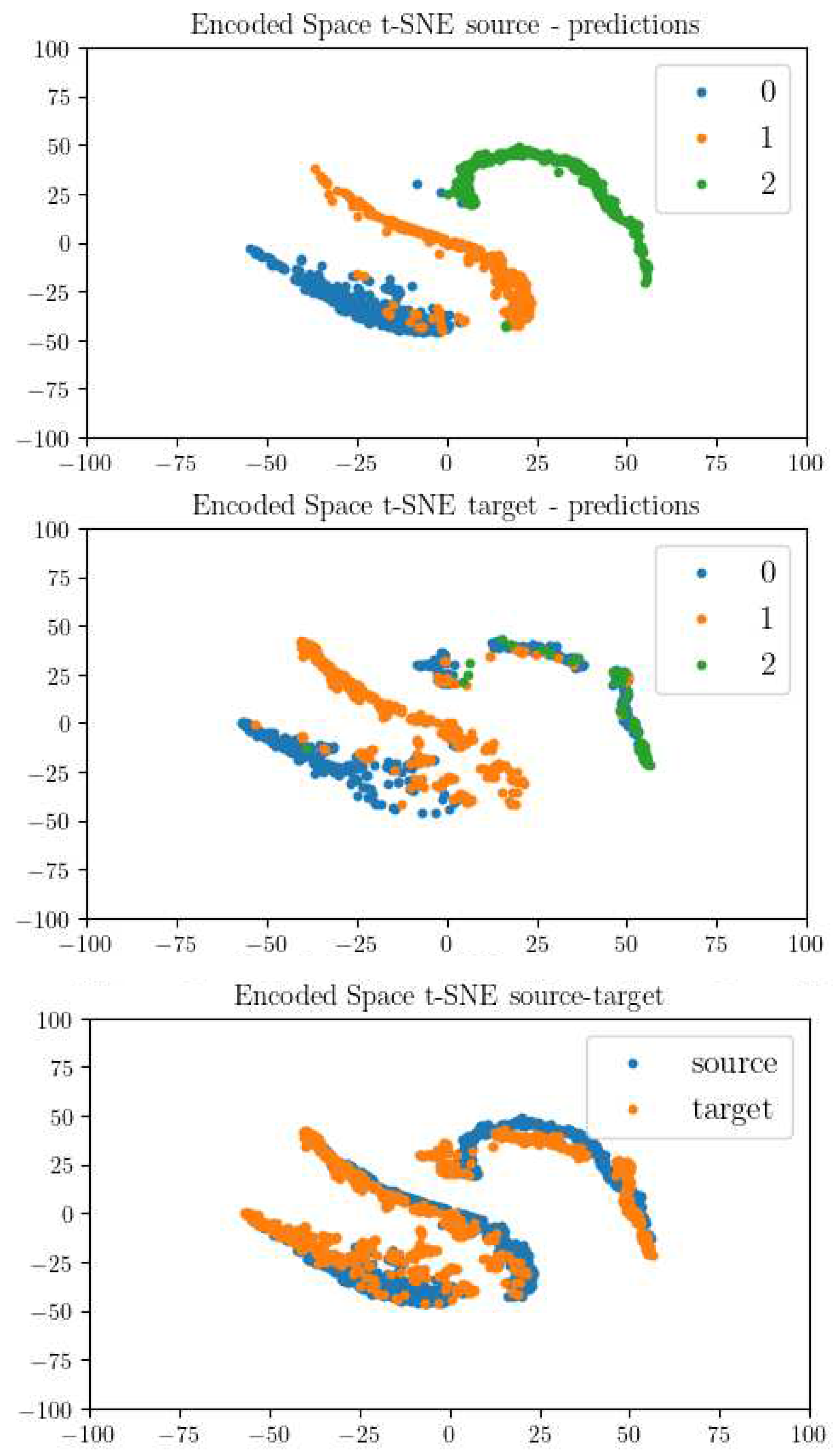
In order to comprehend these results more thoroughly, an analysis of the evolution of the latent features, extracted by the CNN, is conducted when MDD is applied. As demonstrated in Figure 10, three sub-graphs are depicted. The top-left sub-graph represents the projected features extracted from the encoder part of the neural network, utilizing the simulated images. Classification into three categories is derived from the prediction of the NN trained on this data. Conversely, the top-right graph reflects the same process, but is based on the real dataset.

One of the crucial observations is the inability of feature extraction in the real (target) domain to create distinct point sets that enable clear differentiation among the three classes. This failure, which manifests in a significant performance drop when applied to real data, can be traced back to differences between the two domains, a problem the classifier struggles to overcome. Such insights underscore the working hypothesis that domain discrepancies could hamper model performance when shifting from simulated to real data. The bottom graph vividly illustrates this with the non-overlapping simulated (source) and real (target) domains, further reinforcing the classifier’s perception of these domains as two distinct sets.

When MDD is implemented during the training phase, as demonstrated in Figure 12, the outcome is markedly different. It successfully facilitates the extraction of domain-invariant features, thus bridging the gap between simulated and real domains. The points representing these domains align almost identically within the same region, implying an effective decision boundary that classifies data from both domains accurately.

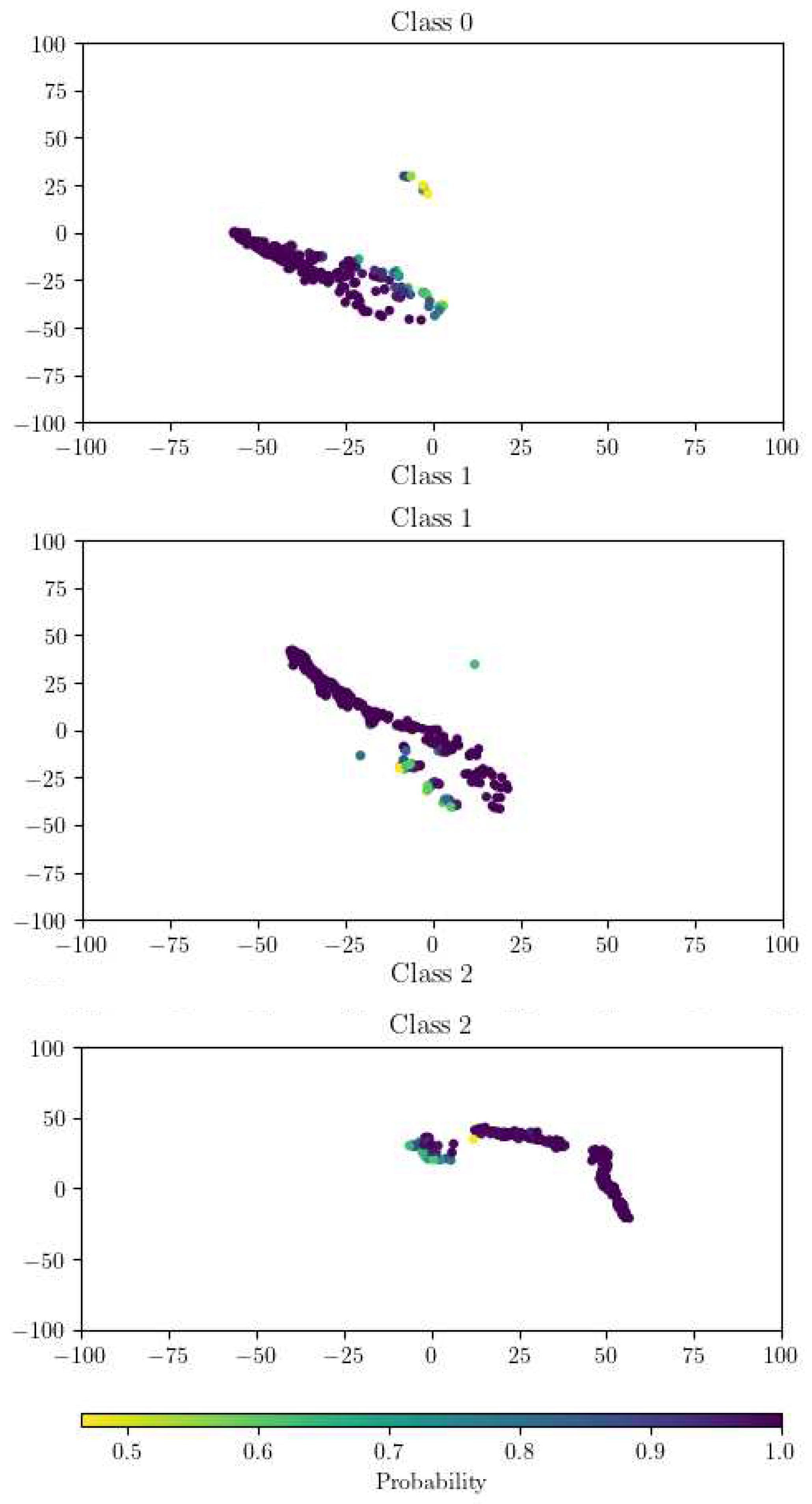
Further improving the quality of results is essential, particularly when considering real-world scenarios where labeling of real data might not be feasible or might be limited due to various constraints. The integration of a Monte Carlo dropout [31] procedure can help address this by modeling the inherent uncertainty associated with the classification task. Figure 11 showcases this, with three sub-graphs exhibiting the t-SNE projection of the latent space for each class in the real domain.

Significantly, the color coding within these graphs corresponds to the classifier’s output probability, which noticeably drops at the boundaries of each cluster where there is a closer proximity between clusters. This visualization highlights the uncertainty at the intersection of class boundaries, and it can guide the refinement of the classifier and the decision process to accept or discard a given prediction.

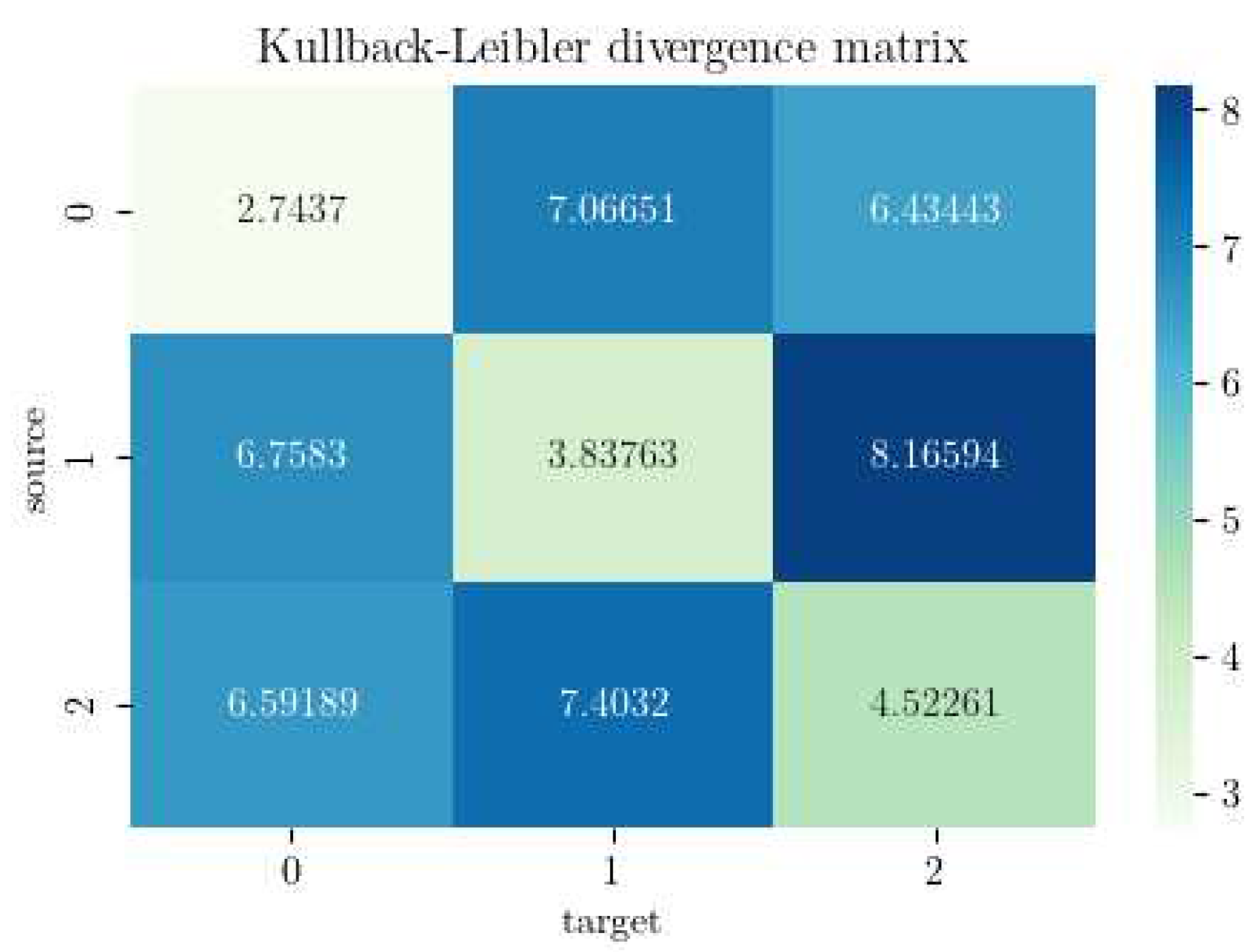
The evaluation of discrepancies between the two domains was further facilitated by the use of a KLD matrix. This tool was utilized to measure the similarity between the three clusters formed in the t-SNE projection. As illustrated in Figure 13, the matrix’s diagonal presents values closer to zero. This outcome indicates greater similarity between the clusters, as anticipated, since these clusters represent the same classes across different domains. However, Class 2 exhibits a higher value compared to Classes 0 and 1. Upon closer examination of the models, we attributed this discrepancy to an error in the model measurements themselves. Future research may seek to investigate and rectify these errors to further optimize model performance across different domains.

5. Conclusions

The discoveries highlighted in this research signify substantial contributions to the domain of SAR image classification when using simulated data, a growing trend in this area. The effective application of Margin Disparity Discrepancy (MDD), the notable improvement in the model’s performance with real data, and the honed discernment of pertinent image features all emphasize the immense value of domain adaptation techniques in augmenting the effectiveness of SAR image classifiers. A key strength of the study lies in the realistic conditions under which the advancements were achieved: real data labels were unavailable, and yet no increase in the model complexity during the inference phase was observed. Moreover, the research did not require an artificial increase in the volume of training data. Consequently, the domain adaptation (DA) approach adopted was entirely unsupervised. This widens its scope of applicability to settings where manual data labeling may be impractical or infeasible, thus demonstrating the resilience and flexibility of such methods. Furthermore, our study lays the groundwork for exciting future research directions. One such avenue involves contrasting the findings of our research with the outcomes from a semi-supervised scenario, wherein a limited subset of data samples is subjected to manual labeling and used in conjunction with simulated data. This comparative approach could provide invaluable insights into the relative merits of supervised, semi-supervised, and unsupervised strategies in various operational scenarios. In doing so, it might unveil novel methodologies for optimizing SAR image classifier performance across diverse contexts. In conclusion, the study has opened up new horizons for enhancing SAR image classification using domain adaptation techniques, offering promising insights for future research in this domain. As we continue to refine these techniques and expand their application, the ultimate aim is to build more robust, efficient, and adaptable SAR image classification systems that can function optimally in real-world scenarios.

Author Contributions

Conceptualization, A.C., A.Q.; methodology, A.C., A.Q.; software, A.C., A.Q., A.P.; validation, A.C., A.Q.; formal analysis, A.C., A.Q.; investigation, A.C., A.Q.; resources, A.C.; data curation, A.C.; writing—original draft preparation, A.C.; writing—review and editing, A.C., A.Q., A.P., T.L. and P.P.; visualization, A.C.; supervision, A.C., A.Q., A.P., T.L. and P.P.; All authors have read and agreed to the published version of the manuscript.

Conflicts of Interest

The authors declare no conflict of interest.

Abbreviations

The following abbreviations are used in this manuscript:

SAR	Synthetic Aperture Radar
AI	Artificial Intelligence
EO	Electro-Optical
CNN	Convolutional Neural Network
UDA	Unsupervised Domain Adaptation
MDD	Margin Disparity Discrepancy
DANN	Domain Adversarial Neural Network
DA	Domain Adaptation
MSTAR	Moving and Stationary Target Acquisition and Recognition
ATR	Automatic Target Recognition
FCN	Fully Connected Network
XAI	Explainable Artificial Intelligence
t-SNE	t-distributed Stochastic Neighbor Embedding
KLD	Kullback-Leibler Divergence
ADAPT	Awesome Domain Adaptation Python Toolbox
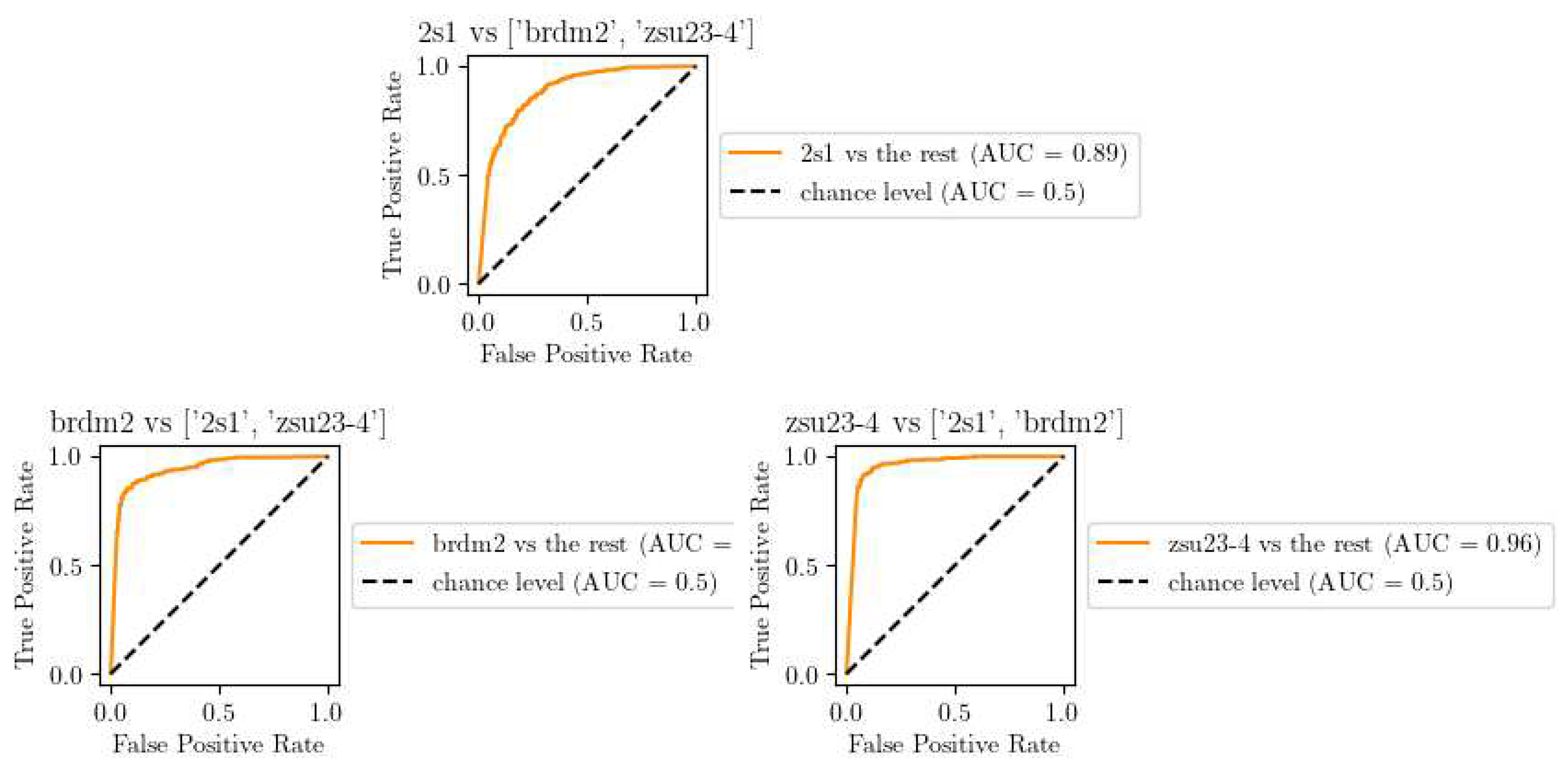
ROC	Receiver Operating Characteristic

References

Huang, M.; Liu, Z.; Liu, T.; Wang, J. CCDS-YOLO: Multi-Category Synthetic Aperture Radar Image Object Detection Model Based on YOLOv5s. Electronics 2023, 12, 3497. [Google Scholar] [CrossRef]
Gromada, K.; Siemiątkowska, B.; Stecz, W.; Płochocki, K.; Woźniak, K. Real-Time Object Detection and Classification by UAV Equipped With SAR. Sensors 2022, 22, 2068. [Google Scholar] [CrossRef] [PubMed]
Sun, Z.; Meng, C.; Cheng, J.; Zhang, Z.; Chang, S. A Multi-Scale Feature Pyramid Network for Detection and Instance Segmentation of Marine Ships in SAR Images. Remote Sens. 2022, 14, 6312. [Google Scholar] [CrossRef]
Yang, X.; Yang, X.; Zhang, C.; Wang, J. SAR Image Classification Using Markov Random Fields with Deep Learning. Remote Sens. 2023, 15, 617. [Google Scholar] [CrossRef]
Liang, W.; Wu, Y.; Li, M.; Cao, Y.; Hu, X. High-Resolution SAR Image Classification Using Multi-Scale Deep Feature Fusion and Covariance Pooling Manifold Network. Remote Sens. 2021, 13, 328. [Google Scholar] [CrossRef]
Zhu, J.; Pan, J.; Jiang, W.; Yue, X.; Yin, P. SAR Image Fusion Classification Based on the Decision-Level Combination of Multi-Band Information. Remote Sens. 2022, 14, 2243. [Google Scholar] [CrossRef]
Rostami, M.; Kolouri, S.; Eaton, E.; Kim, K. Deep Transfer Learning for Few-Shot SAR Image Classification. Remote Sens. 2019, 11, 1374. [Google Scholar] [CrossRef]
G. Ji, Z. Wang, L. Zhou, Y. Xia, S. Zhong and S. Gong, "SAR Image Colorization Using Multidomain Cycle-Consistency Generative Adversarial Network," in IEEE Geoscience and Remote Sensing Letters, vol. 18, no. 2, pp. 296-300, Feb. 2021. [CrossRef]
Guo, Z.; Guo, H.; Liu, X.; Zhou, W.; Wang, Y.; Fan, Y. Sar2color: Learning Imaging Characteristics of SAR Images for SAR-to-Optical Transformation. Remote Sens. 2022, 14, 3740. [Google Scholar] [CrossRef]
Du, Y.; Zhong, R.; Li, Q.; Zhang, F. TransUNet++SAR: Change Detection with Deep Learning about Architectural Ensemble in SAR Images. Remote Sens. 2023, 15, 6. [Google Scholar] [CrossRef]
Li, L.; Ma, H.; Jia, Z. Change Detection from SAR Images Based on Convolutional Neural Networks Guided by Saliency Enhancement. Remote Sens. 2021, 13, 3697. [Google Scholar] [CrossRef]
Shafique, A.; Cao, G.; Khan, Z.; Asad, M.; Aslam, M. Deep Learning-Based Change Detection in Remote Sensing Images: A Review. Remote Sens. 2022, 14, 871. [Google Scholar] [CrossRef]
Lattari, F.; Gonzalez Leon, B.; Asaro, F.; Rucci, A.; Prati, C.; Matteucci, M. Deep Learning for SAR Image Despeckling. Remote Sens. 2019, 11, 1532. [Google Scholar] [CrossRef]
Dalsasso, E.; Yang, X.; Denis, L.; Tupin, F.; Yang, W. SAR Image Despeckling by Deep Neural Networks: from a Pre-Trained Model to an End-to-End Training Strategy. Remote Sens. 2020, 12, 2636. [Google Scholar] [CrossRef]
G. Fracastoro, E. Magli, G. Poggi, G. Scarpa, D. Valsesia and L. Verdoliva, "Deep Learning Methods For Synthetic Aperture Radar Image Despeckling: An Overview Of Trends And Perspectives," in IEEE Geoscience and Remote Sensing Magazine, vol. 9, no. 2, pp. 29-51, June 2021. [CrossRef]
Li, J.; Yu, Z.; Yu, L.; Cheng, P.; Chen, J.; Chi, C. A Comprehensive Survey on SAR ATR in Deep-Learning Era. Remote Sens. 2023, 15, 1454. [Google Scholar] [CrossRef]
Rizaev, I.G.; Achim, A. SynthWakeSAR: A Synthetic SAR Dataset for Deep Learning Classification of Ships at Sea. Remote Sens. 2022, 14, 3999. [Google Scholar] [CrossRef]
F. M. Vieira et al., "Ship detection using SAR and AIS raw data for maritime surveillance," 2016 24th European Signal Processing Conference (EUSIPCO), Budapest, Hungary, 2016, pp. 2081-2085. [CrossRef]
Yan, Z.; Song, X.; Zhong, H.; Yang, L.; Wang, Y. Ship Classification and Anomaly Detection Based on Spaceborne AIS Data Considering Behavior Characteristics. Sensors 2022, 22, 7713. [Google Scholar] [CrossRef] [PubMed]
Woollard, M.; Blacknell, D.; Griffiths, H.; Ritchie, M.A. SARCASTIC v2.0—High-Performance SAR Simulation for Next-Generation ATR Systems. Remote Sens. 2022, 14, 2561. [Google Scholar] [CrossRef]
Zhang, Y. Bridging Theory and Algorithm for Domain Adaptation. In International Conference on Machine Learning. PMLR, 2019, pp. 7404–7413.
Camus, B.; Le Barbu, C.; Monteux, E. Bridging a Gap in SAR-ATR: Training on Fully Synthetic and Testing on Measured Data. IEEE Journal of Selected Topics in Applied Earth Observations and Remote Sensing 2021, 14. [Google Scholar] [CrossRef]
Liang, W.; Zhang, T.; Diao, W.; Sun, X.; Zhao, L.; Fu, K.; Wu, Y. SAR Target Classification Based on Sample Spectral Regularization. Remote Sensing 2020, 12(21), 3628. [Google Scholar] [CrossRef]
Malmgren-Hansen, D.; Kusk, A.; Dall, J.; Nielsen, A. A.; Engholm, R.; Skriver, H. Improving SAR Automatic Target Recognition Models with Transfer Learning from Simulated Data. IEEE Geoscience and Remote Sensing Letters 2017, 14(9), 1484–8. [Google Scholar] [CrossRef]
Zhang, C.; Wang, Y.; Liu, H.; Sun, Y.; Hu, L. SAR Target Recognition Using Only Simulated Data for Training by Hierarchically Combining CNN and Image Similarity. IEEE Geoscience and Remote Sensing Letters, 2022, 1–5. [CrossRef]
Y. Ganin; E. Ustinova; H. Ajakan; P. Germain; H. Larochelle; F. Laviolette; M. Marchand; and V. Lempitsky. Domain-adversarial training of neural networks. In JMLR, 2016. [CrossRef]
The Air Force Moving and Stationary Target Acquisition and Recognition Database. Available online: https://www.sdms.afrl.af.mil/index.php?collection=mstar (accessed on 22/08/2023).
Doerry, Armin. (2019). SAR Image Scaling, Dynamic Range, Radiometric Calibration, and Display. Technical Report No. SAND2022-13587. Available: OSTI Identifier: 1890785.
van der Maaten, L.; Hinton, G. Visualizing data using t-SNE. J. Mach. Learn. Res. 2008, 9, 2579–2605. [Google Scholar]
de Mathelin, A.; Atiq, M.; Richard, G.; de la Concha, A.; Yachouti, M.; Deheeger, F.; Mougeot, M.; Vayatis, N. (2023). ADAPT: Awesome Domain Adaptation Python Toolbox. arXiv e-prints. arXiv:2107.03049. [CrossRef]
Gal, Y.; Ghahramani, Z. Dropout as a Bayesian approximation: representing model uncertainty in deep learning. In Proceedings of the 33rd International Conference on International Conference on Machine Learning - Volume 48 (ICML’16), 2016, pp. 1050–1059.

Figure 1. This figure shows a comparison between CAD models, simulated SAR and MSTAR.

Figure 2. Histogram comparison between real (MSTAR) images (left) and our simulated images (right).

Figure 3. General structure of a DANN.

Figure 4. Accuracy curve of our CNN trained without using Domain Adaptation (DA).

Figure 5. Confusion matrix of our CNN trained without using DA.

Figure 6. ROC curves of our CNN trained without using DA.

Figure 7. Accuracy curve of our CNN trained without using Domain Adaptation (DA).

Figure 8. Confusion matrix of our CNN trained using DA.

Figure 9. ROC curves of our CNN trained using DA.

Figure 10. Split t-SNE finetuning images using DA.

Figure 11. Split t-SNE finetuning using DA.

Figure 12. Split t-SNE finetuning using DA.

Figure 13. KLD matrix of t-SNE.

Table 1. Simulation sensor parameters.

Parameter	Value	Unit
Carrier Frequency	9.5	GHz
Resolution (Range)	0.3	m
Resolution (Azimuth)	0.3	m
Pixel Spacing (Range)	0.2	m
Pixel Spacing (Azimuth)	0.2	m
Thermal Noise	-25	dB

Table 2. Training Configuration

Parameter	Value
Learning Rate	0.0003
Epochs	60
Batch size	32
Optimizer	Adam
Clipnorm	1

Table 3. Training Configuration

Parameter	Value
Learning Rate	0.0003
Epochs	40
Batch size	32
Lambda	[0,1]
Gamma	2
Optimizer	Adam
Clipnorm	1

Disclaimer/Publisher’s Note: The statements, opinions and data contained in all publications are solely those of the individual author(s) and contributor(s) and not of MDPI and/or the editor(s). MDPI and/or the editor(s) disclaim responsibility for any injury to people or property resulting from any ideas, methods, instructions or products referred to in the content.

© 2023 by the authors. Licensee MDPI, Basel, Switzerland. This article is an open access article distributed under the terms and conditions of the Creative Commons Attribution (CC BY) license (http://creativecommons.org/licenses/by/4.0/).

Copyright: This open access article is published under a Creative Commons CC BY 4.0 license, which permit the free download, distribution, and reuse, provided that the author and preprint are cited in any reuse.

MDPI Initiatives

Important Links

Choose an area of interest and we will send you notifications of new preprints at your preferred frequency.

Disclaimer