1. Introduction
Detection of decayed trees is a necessary task for urban greenery managers, park managers or road maintenance personnel. This activity is essential for the early detection of potentially hazardous trees and for preventing injuries, fatalities, or material damages. However, the risk assessment requires experience and time-consuming examination of a tree stem using, e.g. penetrometry, acoustic tomography or electrical impedance tomography [
1,
2,
3,
4,
5]. Methods of tomography may consume around thirty minutes per single tree and are therefore inappropriate for large-scale investigation and at all the potentially hazardous trees. It is also essential to apply the tomography correctly, especially on unevenly shaped trees [
1], because an incorrect measurement may lead to a wrong conclusion and unnecessary removal of a highly valued tree in a park, causing a loss of both esthetical value and shelters for wildlife in an urban area. Even though the tomographic methods are accurate, the final risk assessment still depends on the subjective opinion, producing inconsistency in the estimation [
6]. For these reasons, a faster, easy-to-use, yet reliable and unbiased method would find utilisation in the aforementioned forest management services. The other quality that arborists and forest managers seek is indestructiveness [
5,
7], which could be offered by the proposed method in this study. Even though tomography is considered indestructive [
8], nails are put into the stem during an examination, causing minor wounds to the bark and wood. The method also consumes much time and requires manual labour. That should be avoided by the proposed method, allowing even people without experience in tree risk assessment to estimate tree stem state.
The impact of holes caused by sensors of an acoustic tomograph is not indisputably considered unharmful [
5,
8,
9]. Therefore, it is at hand to develop a technique of internal tree stem decay detection, which definitely is not harmful and produces reliable, unbiased results.
Over the past years, the development of remote sensing has created a new opportunity to make accurate representations of 3D objects and to take advantage of having such a representation for various purposes. In forestry, the most usual utilisation of this data is tree diameter at breast height (DBH), height, volume, or species estimation by both aerial and terrestrial approaches [
10,
11]. While the accuracy of tree DBH estimation has a very low error (3 to 13 mm) [
12,
13,
14], the general presumption for this study is that close. Range photogrammetry (CRP) can accurately reconstruct tree stem shape with all its details and may, therefore, be able to provide a good resource for deep learning and internal tree stem decay detection.
Some studies have examined the possible ways to reconstruct the basal part of a tree using photogrammetry. A practical and intuitive way of imagery collection is sequential imaging while following imaginary circles of 2 and 3 meters in diameter, taking images of a tree stem every few steps [
1,
15,
16]. The number of collected images may vary when using such an approach, but the best results may be expected when each point of the reconstructed object is visible in 8 pictures [
14]. Also, while using CRP, it is necessary to implement any scale bar to scale the 3D reconstruction correctly [
17].
An alternative way of 3D reconstruction is the use of LiDAR. Nowadays, LiDAR sensors are installed in some consumer-grade phones or tablets, which makes the technology more accessible than it used to be. These sensors use the Time-of-Flight method combined with an RGB-D camera, are small and can reconstruct the scene nearly in real-time. On the other hand, its drawbacks are a small reach of 5 to 6 meters and a tendency to misalign repeatedly scanned objects [
18]. This method was already successfully used in forestry research with feasible accuracy for forestry inventory purposes [
19,
20]. A detailed model of each tree stem was not the goal of these studies. Therefore, the accuracy of DBH estimation is not as high as in cited studies using CRP to reconstruct individual trees.
The decay caused by fungi or bacteria is the main reason a tree or its parts fall [
4,
6,
21,
22,
23,
24]. There are two main types of decay in tree stems. Heart rot occurs in the centre of a stem, and sap rot, which starts on the surface, in the sapwood of a stem [
22]. Since heart rot is hard to detect visually, several methods allow to detect a decay based on physical properties, mainly acoustic response or electrical resistivity, impedance respectively [
4,
5,
6]. In this study, only acoustic tomography was used to detect the actual health state of trees. This method is based on measuring the time of flight of sound waves [
5]. Generally, the stress wave propagates faster in dense and healthy wood, whereas the decayed wood results in a much slower stress wave propagation as the stress wave needs to bypass holes and gaps created by the decay [
25]. The time is measured using a timer and a series of accelerometers placed on a stem at the same height level. These sensors require metal nails to be knocked into the wood. As soon as a stress wave is emitted from one accelerometer by a hammer tap, the time of flight is measured for each of the receiving accelerometers. Afterwards, the same process is done for all the other accelerometers [
5,
26]. The alternative methods for tree stem decay detection are electrical impedance tomography, which measures electrical conductivity in the wood, where healthy wood has a higher resistivity than decayed wood due to its wetness [
2,
5], and resistance drills, which measures the power needed to drill through a piece of timber thus indicates its state [
3,
5].
In practical use, the stem shape is often simplified and replaced by a circle or cylinder shape, leading to an incorrect estimation of sensor-to-sensor distances and distortion of the outcome tomogram. Previous studies verified that sensor locations may be detected on 3D photogrammetric models with very high precision, and calculation of the exact distances of sensors from each other for tomography is possible [
1,
17,
27]. A similar procedure of sensor location estimation will be described in the proposed study as well. Some of these studies also attempted to overcome a standard limitation of tomography. The method can only show the status of wood in a 2D cross-section. Multiple sections must be examined to obtain a more precise representation of the whole stem base, which requires a significant amount of time. The mentioned studies attempted to reconstruct the state of decay in the entire stem base using multiple cross-sections of tomography and interpolation between them, resulting in a complete model of the inner stem state [
1,
17]. However, the result is only an estimate based on several 2D cross-sections and might not improve the ability of correct risk assessment.
A new trend in data evaluation is the use of deep learning. Usually, images or 3D point clouds are often evaluated by neural networks, and exciting results are reported in object detection or classification. Specifically in the detection of individual trees or tree species classification [
28,
29,
30,
31], but it is appropriate for the detection of any feature with distinctive patterns [
32]. For 3D data classification, the PointNet deep learning algorithm is often used [
28,
31,
33,
34], and due to its satisfactory performance, it was also used in this study to evaluate 3D meshes or point clouds respectively and classify them into one of the desired classes, where the input data contain 3D models of standing tree stems, scanned in urban greenery by both close-range photogrammetry and iPhone LiDAR. The algorithm used for point cloud classification in the proposed study is PointNet. The algorithm works directly with unordered 3D point clouds and is invariant to geometric transformations of the point cloud. It is suitable for object classification, segmentation or semantic parsing [
35].
In some studies, the need to process a point cloud directly was bypassed by using other interpretations of point clouds, such as images or snapshots from varying views, which leads to processing 2D data with satisfying results and accuracy higher than processing 3D data [
33,
36].
By combining terrestrial remote sensing and deep learning, the proposed work aims to reconstruct basal parts of standing tree stems and their classification based on the decay state inside the tree stem, which was estimated using acoustic tree stem tomography. This study should represent a low-cost and well-accessible approach to close-range remote sensing and object classification problems in arboriculture or forestry. The proposed method introduces a novel way of tree health evaluation. Therefore, the methods used should be accessible to most enterprises potentially interested in this method.
2. Materials and Methods
2.1. Study Site
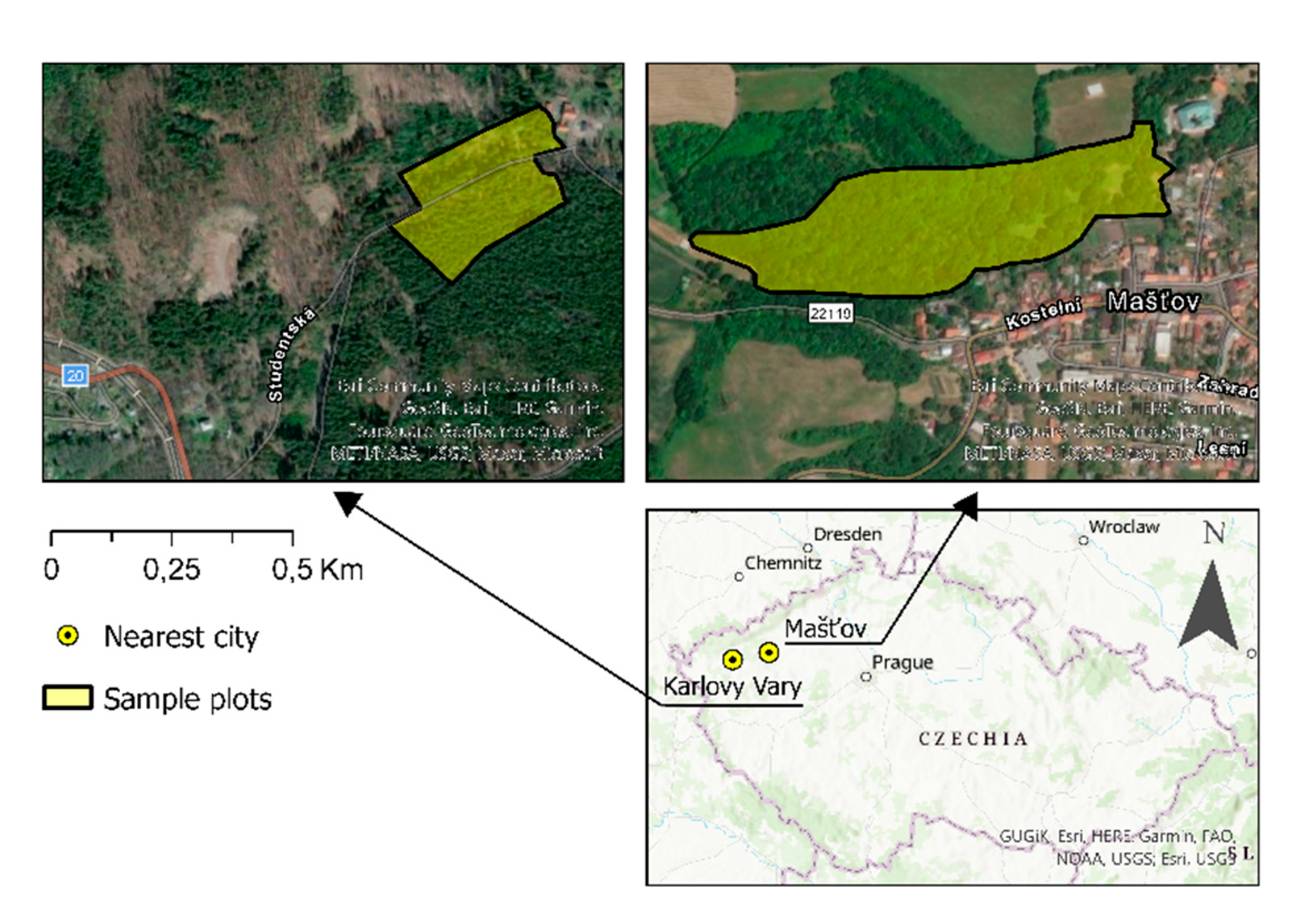
The data collection was conducted at two locations. The first location, lying at an altitude around 510 MSL, is property of the enterprise Lázeňské lesy a parky Karlovy Vary PBC and lies in its rope climbing park Svatý Linhart, on the southern edge of the city of Karlovy Vary. This area is a mature, managed, even-aged European Spruce forest with a moderate European Beech understory and stocking density of 0.9 [
37]. The soil type is Dystric Cambisol on the primary granite rock [
38,
39]. The mean yearly temperature is between 8 and 9 °C, and the mean annual precipitation ranges from 600 to 700 mm [
40].
The second study site is related to the town Mašťov, 30 kilometres east of Karlovy Vary. The object of interest was an old and unkept castle park associated with the local palace. Above sea altitude of the area is around 400 MSL, and the climatological data are the same as in the first study site [
40]. Regarding geology, this site is composed of vulcanite and sedimental layers. Present soil types are eutrophic cambisol and gleyic fluvisol [
38,
39]. Present tree species are mainly Acer pseudoplatanus, Acer platanoides, Quercus robur, Alnus glutinosa and Fraxinus excelsior in the main level and understory. The forested area of the park is fully stocked with rich understory.
Figure 1.
Locations of study plots southerly from the city of Karlovy Vary and northerly from the town of Mašťov.
Figure 1.
Locations of study plots southerly from the city of Karlovy Vary and northerly from the town of Mašťov.
2.2. Data Collection
In the period from April 2023 until October 2023, fieldwork took place. During this time, trees of varying species were selected, primarily based on large DBH, as thick trees are potentially the most dangerous and were closely examined. A workflow was conducted on each tree, providing RGB imagery for further photogrammetric processing, iPhone LiDAR point cloud and up to four tomograms from various stem heights obtained by acoustic tomography.
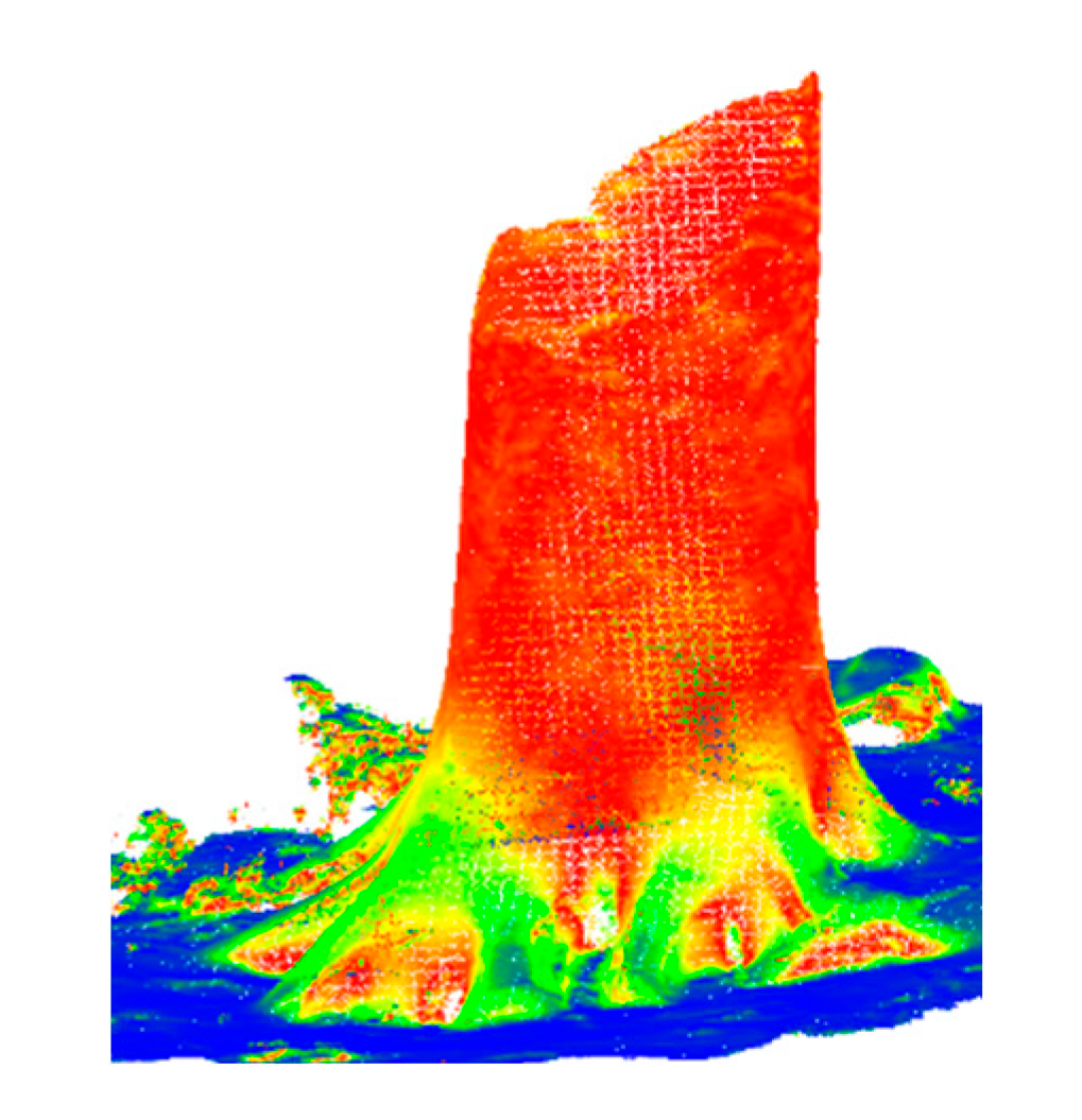
Figure 2.
iPhone Lidar point cloud. Colours depict Verticality: 0 (Blue) to 1 (Red).
Figure 2.
iPhone Lidar point cloud. Colours depict Verticality: 0 (Blue) to 1 (Red).
Firstly, images for CRP were collected using an iPhone 12 Pro RGB camera with the Lens Buddy app [
41], allowing users to collect sequential images at predefined quality. In the case of the proposed study, the interval was set to one second, and the photo output format was DNG. Other parameters of the app settings are described in
Table 1. These images aimed at getting a clear view of the basal part of a tree stem up to the height of approximately 3 meters and, simultaneously, depiction of printed paper scale bars, exported from Agisoft Metashape [
42], which were placed on certain spots around the stem base. Photographs were taken on a circular trajectory, which consisted of two circles. The first circle was approximately 3 meters in diameter and aimed at capturing the stem and all paper scale bars. The second circle was smaller and aimed mainly at capturing the stem itself. In total, there were about 70 pictures taken for each tree, which is given by the fact that saving images in the RAW format is slow, and the phone cannot keep up with the one-second interval per each image taken.
Secondly, iPhone LiDAR scanning was conducted using the LiDAR sensor of the iPhone 12 Pro. For this purpose, the 3d Scanner App [
43] was used. It was set to the LiDAR Advanced mode, and the further app settings are shown in
Table 1. This scanning was made on a single circular trajectory, very close to the stem. For a good result, the iPhone had to be held parallel to the ground, display facing up, and follow a wavy trajectory to reconstruct both the higher and lower parts of the stem. This way, the stem up to the height of 2.5 meters could have been scanned. The created point cloud was exported from the app in LAS format and at a high density of points.
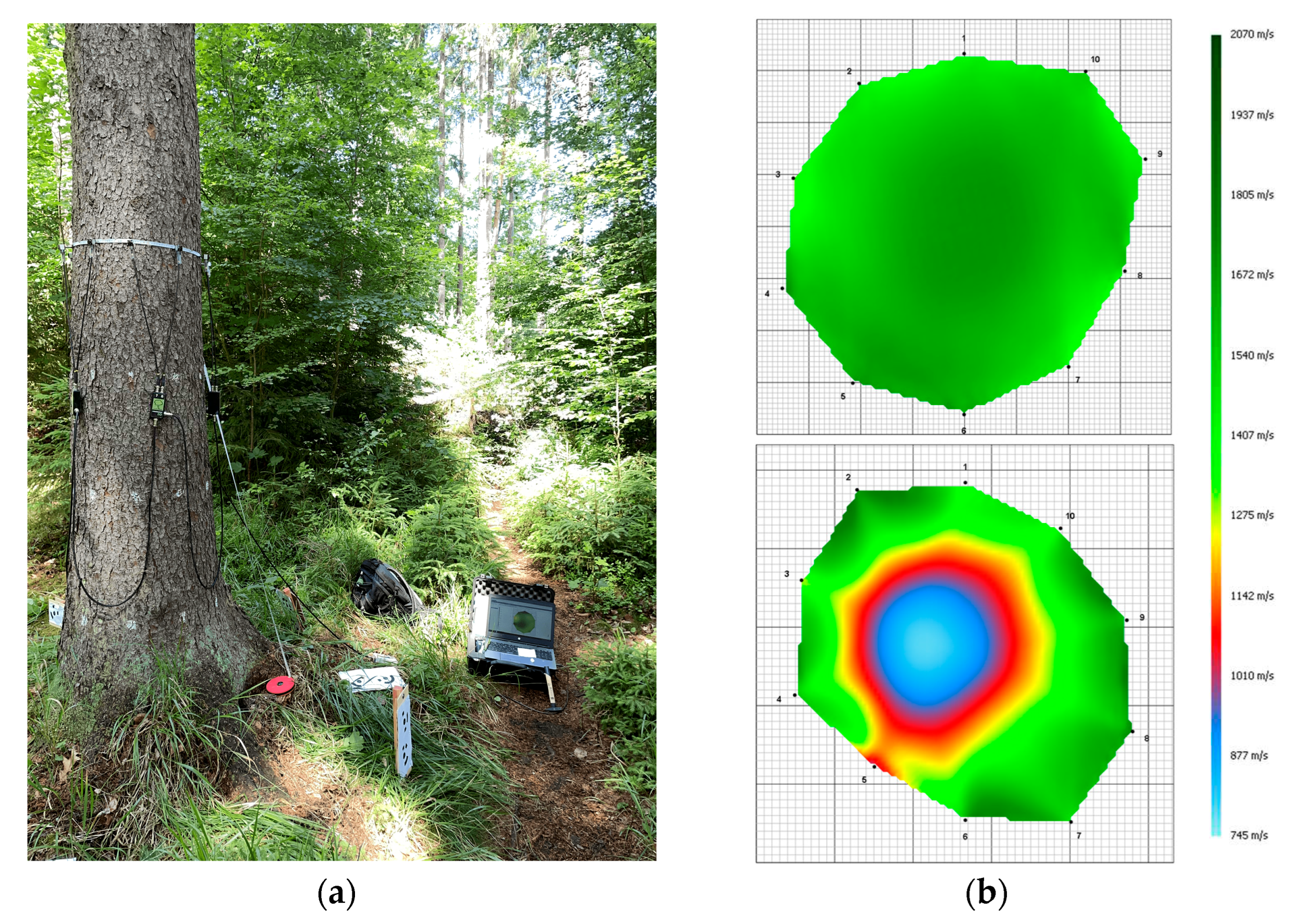
As the third step, acoustic tomography took place. The device and software ArborSonic 3D [
44], produced by Fakopp Enterprise Bt., was used. Each time, ten sensors were put equally around the tree stem. The first one was placed on the northern side of the stem, and the following sensors were placed in the counterclockwise direction. Further, the instructions of the manufacturer were followed. The tomography was conducted in up to four height levels, from 0.5 meters to 2 meters, if possible. After the entire procedure, spots where the sensors were nailed in were marked with white chalk. For simplicity, the stem shape was considered a circle, but this drawback was resolved in later processing, obtaining an accurate representation of tree stem shape and sensor distances with the help of marks made by the chalk and accurate photogrammetric models.
Figure 3.
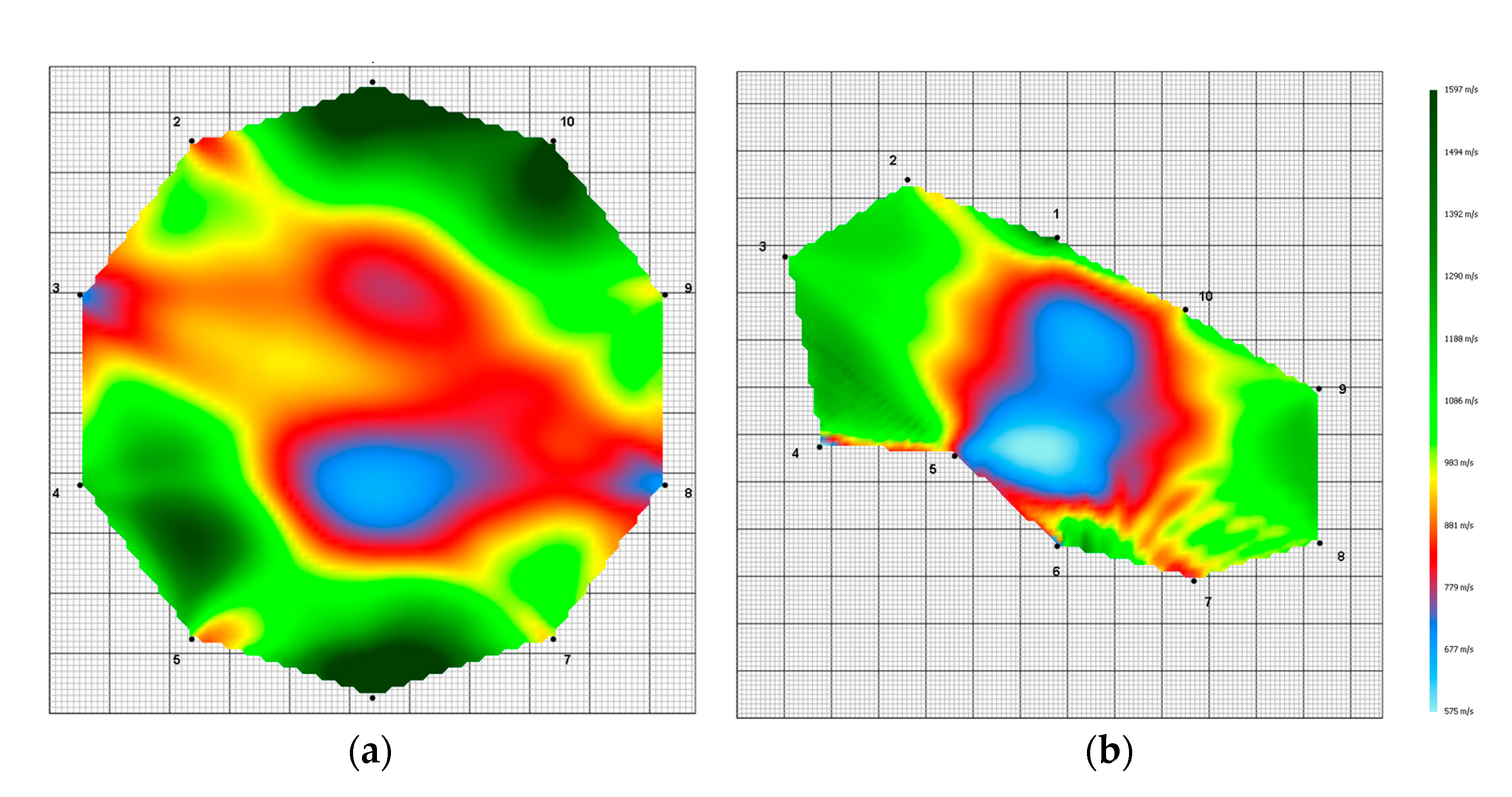
(a) Acoustic tomograph Arbor Sonic 3D; (b) Tomograms of a healthy and decayed stem.
Figure 3.
(a) Acoustic tomograph Arbor Sonic 3D; (b) Tomograms of a healthy and decayed stem.
The last step was practically the same as the first step, where images for CRP were collected. This second imaging aimed to obtain a 3D representation of a stem with the locations of tomograph sensors, now marked by white chalk, which was used to highlight these locations and, unlike paper markers, does not occlude the actual shape of the stem.
2.3. Data Processing
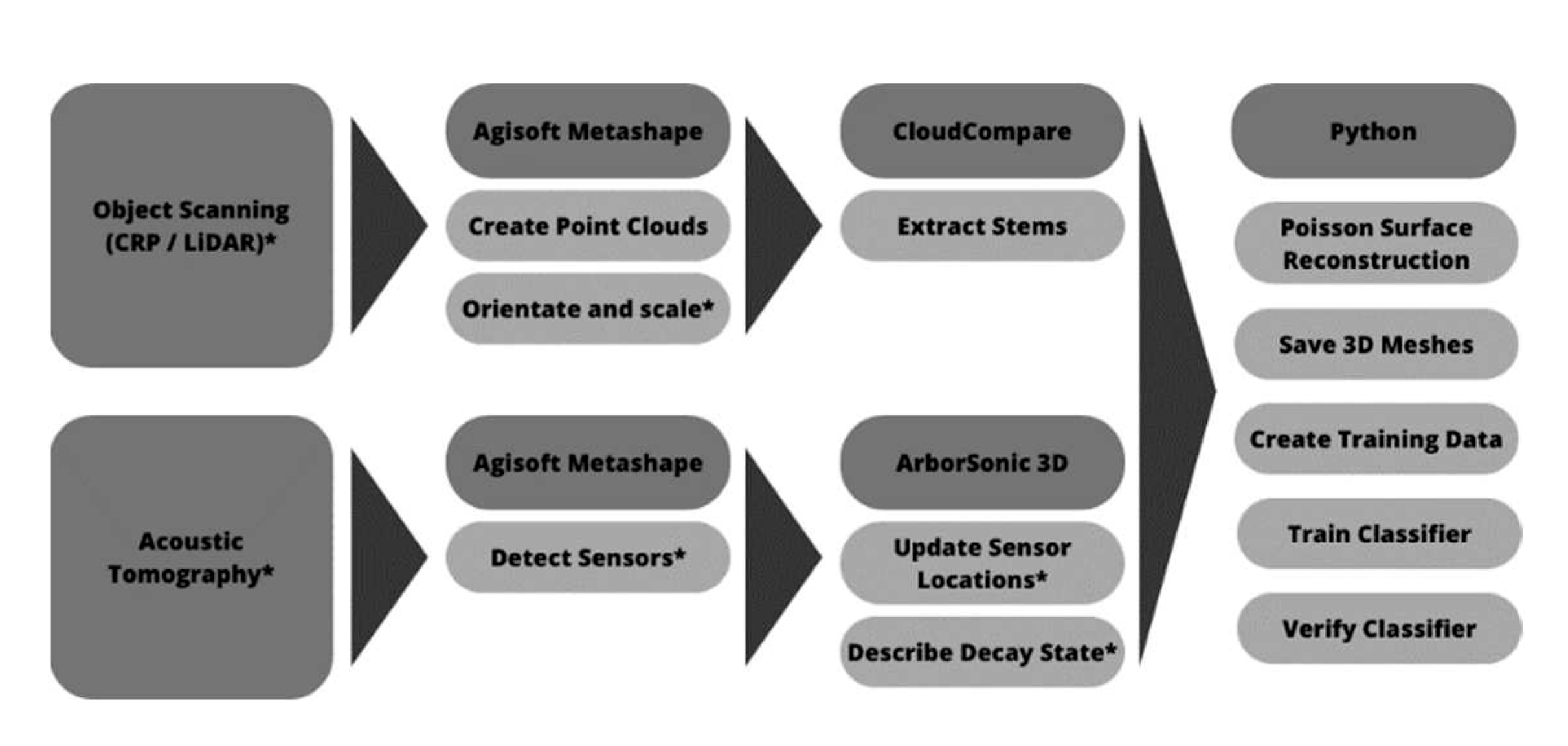
The data processing followed several main steps, described in
Figure 4. The task was to create as precise models of scanned tree stems as possible, without any other objects in the scan, label the trees according to the state of decay in the stem and use these models as learning and validation data for PointNet training.
The images for CRP were processed using Agisoft Metashape software and were turned into 3D Point Clouds using basic workflow. Scale bars had to be manually added in the created dense point clouds using the automatically detected markers. Distances among the detected paper markers were known and could have been defined in the software as well. As soon as the point clouds were scaled, it was necessary to manually orientate them correctly to make the Z axis follow the axis of each stem. This is necessary for further automated processing of point clouds.
Figure 4.
Basic workflow of the data processing. The asterisk indicates steps that had to be done manually.
Figure 4.
Basic workflow of the data processing. The asterisk indicates steps that had to be done manually.
In the point clouds made of images taken after tomography and containing marked tomograph sensor locations, white chalk points have been manually detected and marked by markers in Agisoft Metashape software. As soon as this procedure was done, the local coordinates of sensors were exported for each tree and used to calculate accurate distances among sensors. There were ten sensors in each examined cross-section on the tree stem. If the circumstances did not allow conducting tomography in four levels, a lower number of levels was measured. Sensor distances were calculated using a Python script that implemented the formula for calculating distances in 3D space:
The distances were later entered manually into the ArborSonic 3D projects, replacing the distorted values collected in the field when the stem shapes were only considered a circle, as visible in
Figure 5.
Once the tomograms representing decay were more accurate, a file containing information about each tree, mainly Tree ID, Genus, Species, Decay Severity, and other less essential parameters, was created. The Decay Severity was determined based on tomograms subjectively and expresses the amount of decay in the tree stem on a scale from 0 to 3, where 0 corresponds to no decay, 1 to very small decay, 2 to substantial decay and 3 to massive decay. These values served later as labels for the neural network training.
Figure 5.
(a) Tomogram before adjustment; (b) Tomogram after adjustment by calculating more accurate sensor distances.
Figure 5.
(a) Tomogram before adjustment; (b) Tomogram after adjustment by calculating more accurate sensor distances.
The following steps are done automatically based on a Python script, which processes all point clouds of desired tree species into a 3D mesh, filtering out the terrain and other objects, keeping only the stem of interest.
For this purpose, the Verticality feature is calculated based on the normals of the point cloud, allowing for accurate distinction between terrain and stem, as horizontal surfaces have the value Verticality equal to zero and vertical equal to 1. This feature is shown in
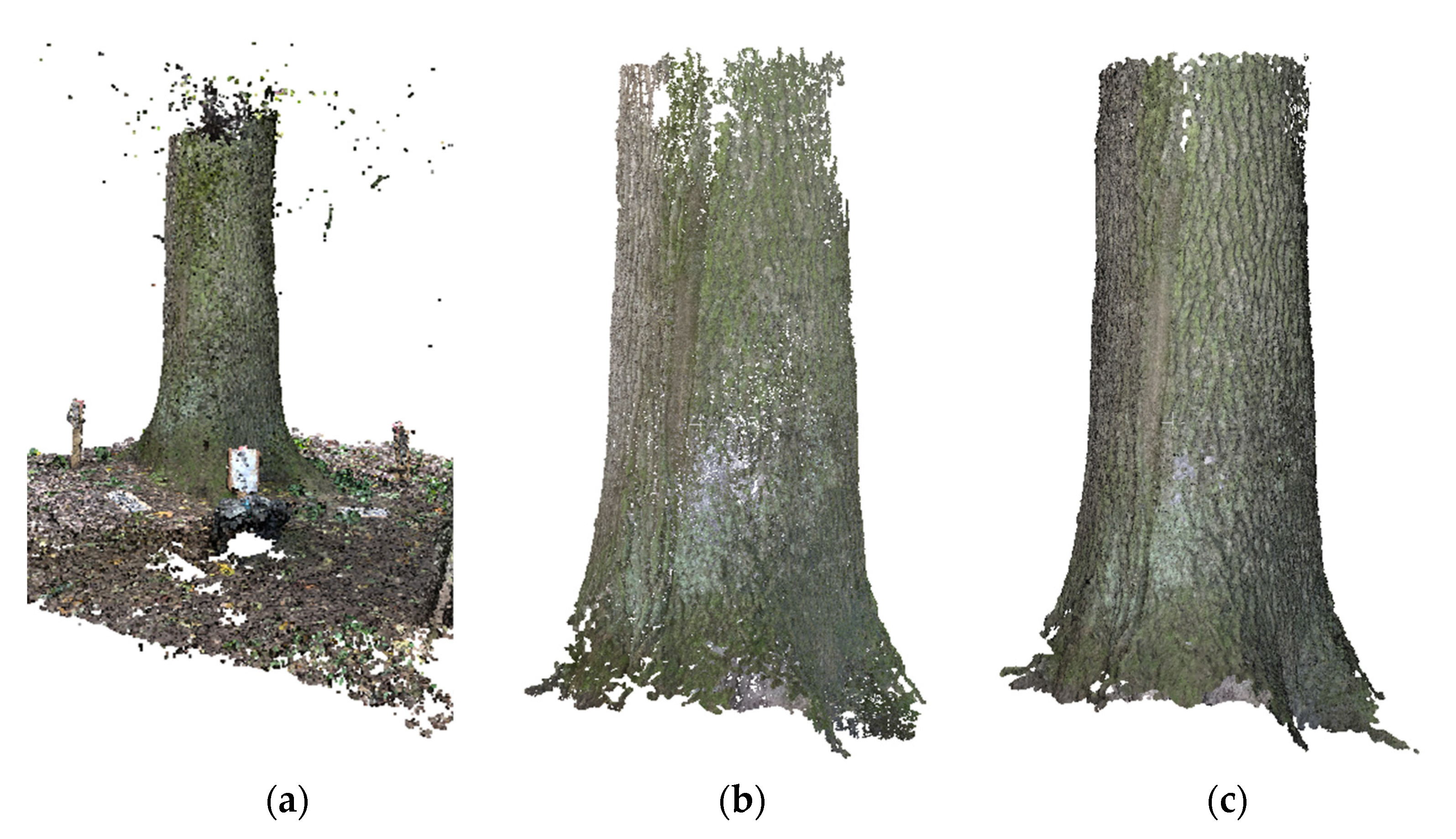
Figure 2. In case normals were absent, which was the case of iPhone LiDAR data, these had to be estimated using the Octree Normals function in Cloud Compare's Command Line mode. Tress usually can be separated from terrain by keeping points with Verticality between approximately 0.6 and 1.0. Another step is necessary as the filtering based on Verticality does not remove all unwanted points from the original point cloud. This procedure makes use of the CloudCompare function named Label Connected Components, which detects clusters of points at a defined level of rigour. Usually, small features are parts of terrain or noise, whereas the most extensive feature is mostly the woody part of a stem and is separated from all the other points, resulting in a separated stem and terrain.
The filtered stem point cloud is then turned into a 3D mesh using Poisson Surface Reconstruction, which solves the reconstruction as a spatial Poisson problem, considering all present points simultaneously, unlike other methods. This surface reconstruction method allows for robust reconstruction of real-world objects from a point cloud into a 3D mesh, even if the input point cloud is highly noisy. However, the input point cloud must contain normals; otherwise, the algorithm would not work. The normals are used for the so-called Indicator Function and its Gradient, which detects points belonging to the object, its surface and noise [
45]. A brief overview of the point cloud processing is visible in
Figure 6.
The meshes serve as input data for the PointNet neural network, which firstly plots a certain amount of points onto the mesh and creates a new point cloud this way. The original point clouds from iPhone LiDAR and close-range photogrammetry cannot be used, as all input point clouds must have the exact same number of points.
PointNet trains a classifier based on labelled 3D meshes and predefined hyperparameters: the number of points sampled on the 3D mesh, batch size, number of epochs and learning rate. The selection of proper hyperparameters is a crucial part of deep learning classifier training and is described further in the text.
Filtering a tree stem was done using the Command line mode of CloudCompare software [
46]. Its functions, namely the Verticality feature and the Label Connected Components function, were embedded in the mentioned Python code.
The other parts of the Python code were done using freely accessible libraries such as open3d, tensorflow, keras, numpy, os, shutil and others. Poisson surface reconstruction was conducted using the open3d library, providing quick and satisfactory data processing.
The final step is the PointNet processing, which requires the determination of well–performing hyperparameters, which is done iteratively by the method of Grid Search [
32], described in the following section.
Figure 6.
(a) Original CRP Point Cloud (b) Automatically separated stem (c) 3D Mesh of the stem.
Figure 6.
(a) Original CRP Point Cloud (b) Automatically separated stem (c) 3D Mesh of the stem.
2.4. Data Analysis
Analysis of tree stem models was done by a slightly updated version of the PointNet algorithm [
35], trying to classify trees into either the Healthy class or Decayed class, substituted by the dummy values 0 or 1. This was done due to insufficient samples for training a four-class classifier. Due to the algorithm's invariance to geometric transformations, it is not possible to synthetically extend the dataset by simply rotating, resizing or moving the input point clouds, and for that reason, the dataset could not have been extended in this manner. Therefore, Point clouds were slightly modified during the PointNet algorithm processing, moving each point slightly by a randomly selected value equal to up to 5 millimetres in any direction.
There were three kinds of classifiers created. One for the Coniferous trees decay classification, consisting of European Spruce models. The second one is for the Deciduous tree species decay classification, containing Fagus sylvatica, Fraxinus excelsior, Acer platanoides, Acer pseudoplatanus and Quercus robur, and the third one is for a mix of all the aforementioned tree species with other tree species, that were marginally examined during the fieldwork.
For proper training, optimal hyperparameters had to be chosen by an iterative approach of Grid Search. This approach requires a user-defined set of values that shall be examined. As all possible preset hyperparameter values are processed, this approach is only suitable for cases with approximately three or fewer hyperparameters to be examined. The input values have to be set based on prior experience and respecting results of previous stages of the Grid Search to save computational resources, as these are already heavily exploited with the iterative approach and may grow exponentially by adding new examined hyperparameters into the search [
32]. Therefore, a matrix of potential hyperparameters was made, and the training was run with every possible combination of these. As the variation of validation accuracy varied significantly, even if the same input parameters were used, each combination was run one hundred times to state a mean performance of the validation confidently. The modified hyperparameters were Batch Size, Point Number, Epochs and Learning Rate, and most of the time was spent tweaking the number of epochs, which defines how many times the data will be seen by the PointNet algorithm before the training finishes. The batch size, on the other hand, defines how many point clouds from the overall dataset will be used by the algorithm for training at one time. This number cannot be too high, as the computational resources of a PC may not suffice, but it also needs to be as high as possible, as it improves the final classifier's accuracy. The number of points defines how many points will be plotted on a 3D mesh, creating a point cloud. Lastly, the learning rate, which determines the size of the steps taken during the optimisation process, requires a fair amount of attention. It is a critical parameter because it influences how quickly or slowly a neural network learns. A very high learning rate causes faster training but with a risk of missing the best solution to its large modifications in the model's parameters. In opposition, a very low learning rate causes slow training, and optimisation may get stuck in a local minimum, preventing it from reaching the total minimum, i.e., the optimal solution [
32,
47].
In order to verify that the PointNet training program itself works well, the training and validation were also conducted on the ModelNet10 benchmark dataset with appropriate hyperparameters and a validation accuracy of 90 %.
3. Results
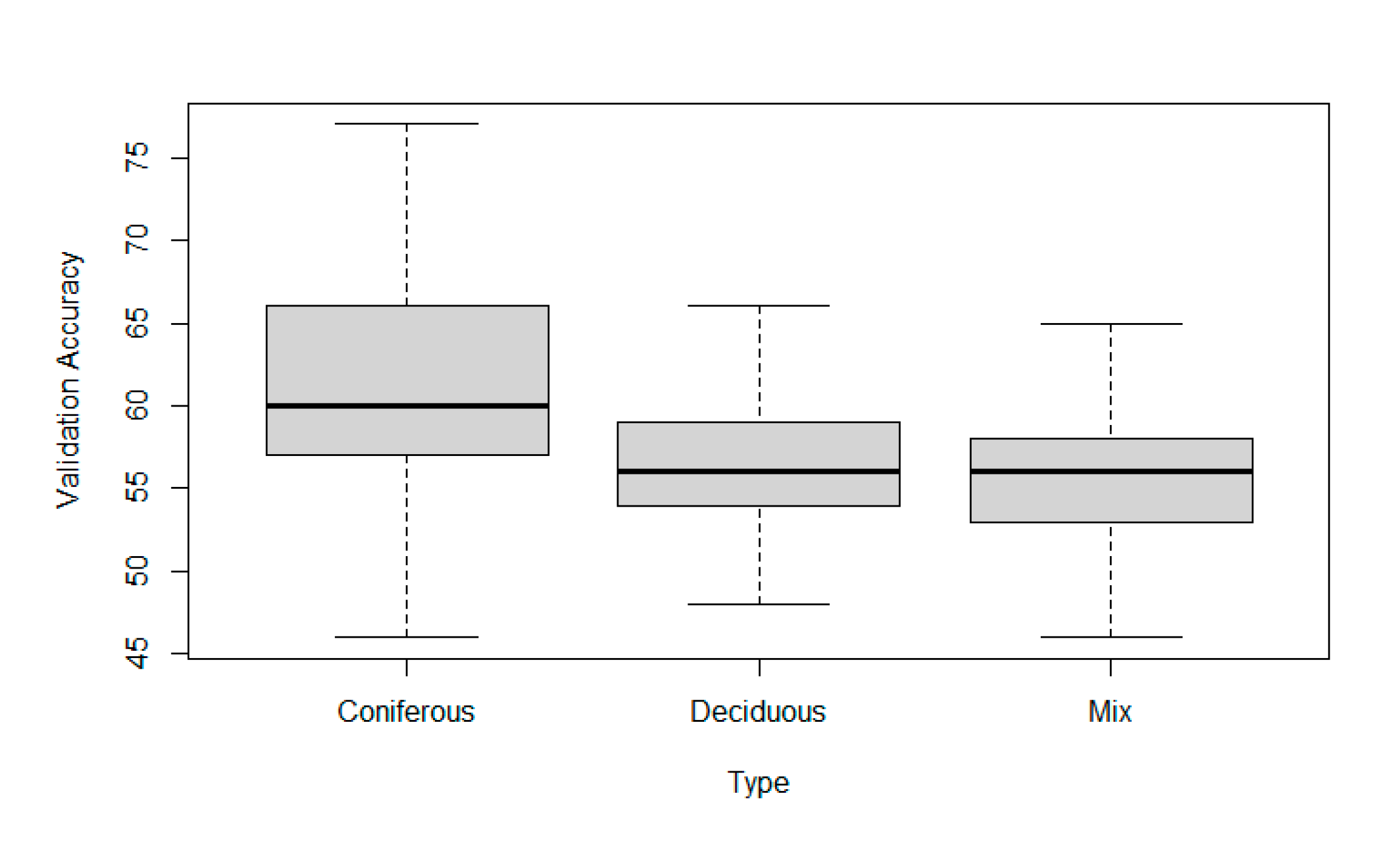
The performance of the PointNet classifier for decayed tree detection was demonstrated on a validation set extracted from the original dataset. However, it has demonstrated that the accuracy of the best classifiers in mean reaches approximately 65 % for Coniferous, 58 % for Deciduous and 58 % for Mixed data, as visible in
Figure 7. Therefore, it was verified that the internal state of a tree stem could be, to some extent, deduced by deep learning methods, and this approach may be later helpful in practical use. However, as this application is in the initiation phase, more similar experiments are necessary.
Figure 7.
The representation of validation accuracy changes with the type of data used. Other parameters are kept as described in the text.
Figure 7.
The representation of validation accuracy changes with the type of data used. Other parameters are kept as described in the text.
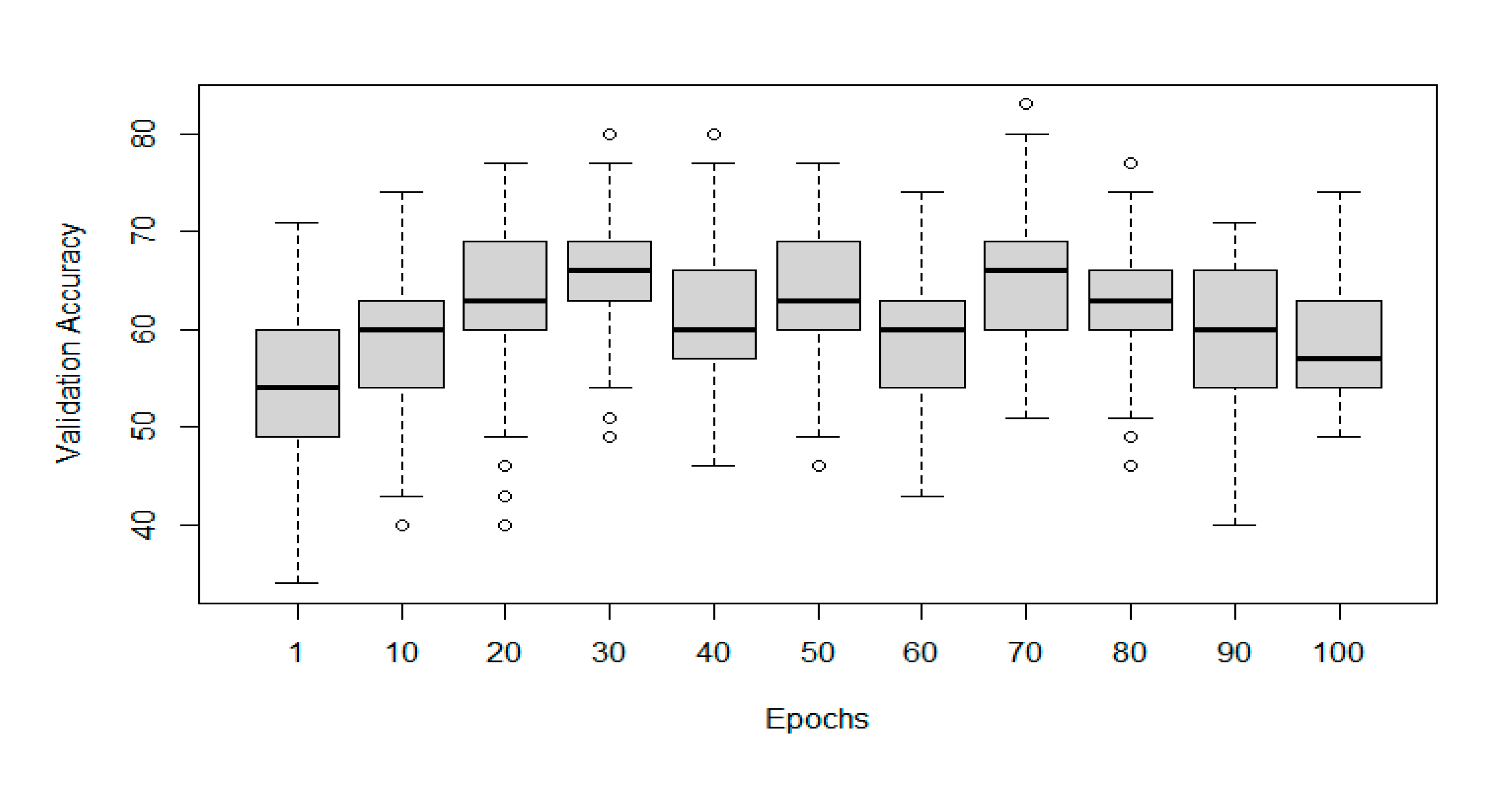
Table 2 represents varying results of Coniferous stems classifiers, which were trained and tested on a dataset consisting of 180 3D meshes, out of which 69 represented healthy trees with no decay and 111 with varying states of decay from slight to massive rot. Out of the total, 35 meshes were used for validation. The best performance was shown using the following hyperparameters for the PointNet function: number of points = 2048, batch size = 32, learning rate = 0,001 and number of epochs = 30 or 70. For each combination of hyperparameters, 100 iterations were made to eliminate speculation that the positive results were obtained by chance. The course of validation accuracy and its dependence on the number of epochs is shown in
Figure 8.
Table 2.
Properties of validation accuracy of Coniferous model with batch size equal to 32, obtained based on 100 iterations of the classifier training. The best results are highlighted.
Table 2.
Properties of validation accuracy of Coniferous model with batch size equal to 32, obtained based on 100 iterations of the classifier training. The best results are highlighted.
| Epochs |
Mean |
St. Dev. |
Mode |
Min |
Max |
| 1 |
55,2 |
7,4 |
54 |
34 |
71 |
| 10 |
59,1 |
7,2 |
63 |
40 |
74 |
| 20 |
63,5 |
7,5 |
60 |
40 |
77 |
| 30 |
65,5 |
6,2 |
66 |
49 |
80 |
| 40 |
60,3 |
6,8 |
60 |
46 |
80 |
| 50 |
63,5 |
6,5 |
63 |
46 |
77 |
| 60 |
59,1 |
6,4 |
60 |
43 |
74 |
| 70 |
65,4 |
7,1 |
66 |
51 |
83 |
| 80 |
62,2 |
6,0 |
60 |
46 |
77 |
| 90 |
59,3 |
6,9 |
60 |
40 |
71 |
| 100 |
58,6 |
5,7 |
57 |
49 |
74 |
Figure 8.
The representation of validation accuracy changes with the number of epochs on the Coniferous dataset. Other parameters are kept as described in the text.
Figure 8.
The representation of validation accuracy changes with the number of epochs on the Coniferous dataset. Other parameters are kept as described in the text.
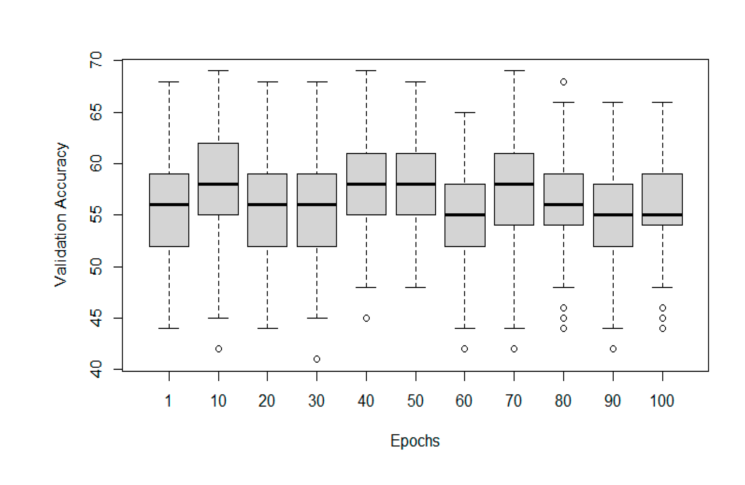
Table 3 describes the results of Deciduous tree stem classifiers, which worked with a dataset of 355 3D meshes. Of them, 205 represented healthy trees with no decay and 150 with varying decay from slight to massive rot. For validation, 71 meshes were used. The best performance was shown while using the following hyperparameters for the PointNet function: number of points = 2048, batch size = 32, learning rate = 0,001 and number of epochs = 40, which is also indicated by
Figure 9.
Table 3.
Properties of validation accuracy of Deciduous model with batch size equal to 32, obtained based on 100 iterations of the classifier training. The best results are highlighted.
Table 3.
Properties of validation accuracy of Deciduous model with batch size equal to 32, obtained based on 100 iterations of the classifier training. The best results are highlighted.
| Epochs |
Mean |
St. Dev. |
Mode |
Min |
Max |
| 1 |
56,1 |
5,1 |
59 |
44 |
68 |
| 10 |
58,4 |
4,4 |
61 |
46 |
69 |
| 20 |
55,1 |
5,2 |
55 |
44 |
68 |
| 30 |
56,8 |
4,5 |
58 |
41 |
68 |
| 40 |
58,4 |
3,6 |
58 |
51 |
68 |
| 50 |
58,4 |
3,8 |
56 |
49 |
68 |
| 60 |
54,9 |
3,6 |
56 |
44 |
62 |
| 70 |
57,3 |
4,1 |
58 |
42 |
69 |
| 80 |
58,5 |
4,0 |
56 |
46 |
66 |
| 90 |
54,3 |
4,4 |
54 |
42 |
66 |
| 100 |
57,5 |
3,3 |
55 |
45 |
66 |
Figure 9.
Representation of the validation accuracy change with changing number of epochs on the Deciduous dataset. Other parameters are kept as described in the text.
Figure 9.
Representation of the validation accuracy change with changing number of epochs on the Deciduous dataset. Other parameters are kept as described in the text.
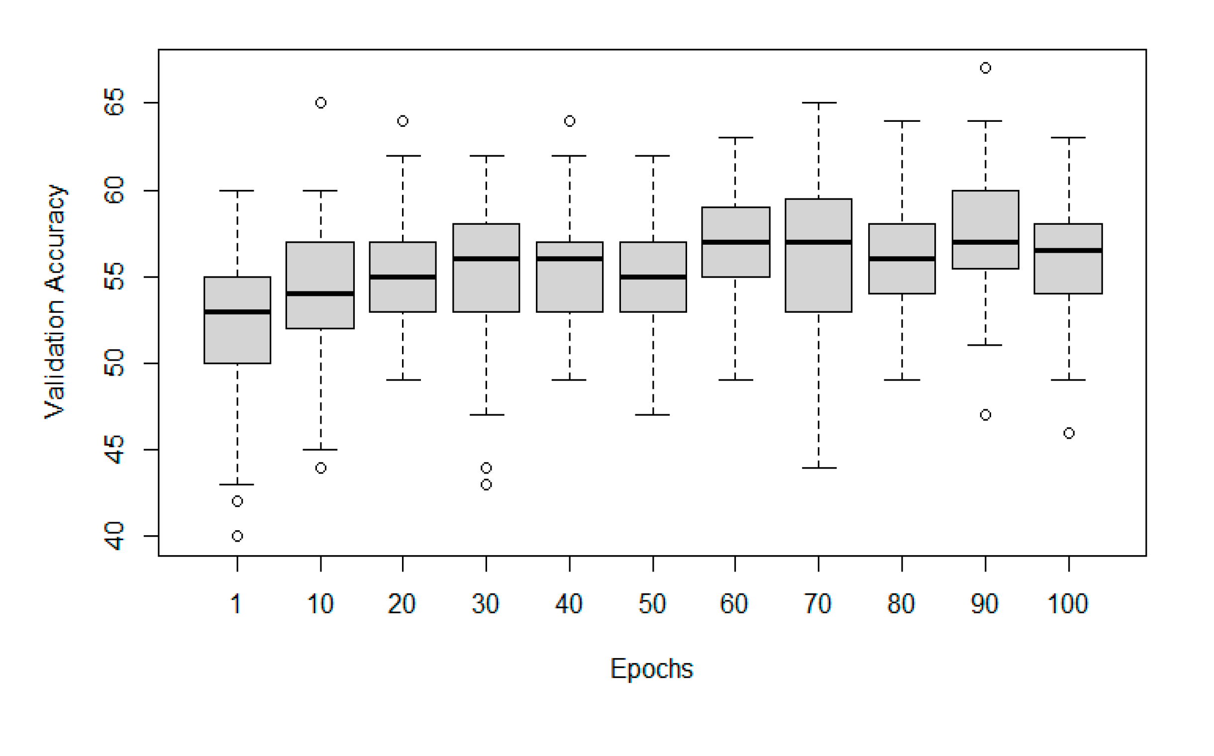
Table 4 presents the accuracies of Mixed stems classifiers, consisting of merged datasets of Coniferous, Deciduous and other tree species that were marginally examined during the fieldwork, consisting of 15 tree species and 649 3D meshes. One hundred twenty-nine meshes were used for the validation. As visible in
Table 4 and
Figure 10, the best-performing training hyperparameters for this case were number of points = 2048, batch size = 32, learning rate = 0,001 and number of epochs = 70.
The results are of promise that further work may reveal the higher potential of this method and make the predictions more reliable.
Table 4.
Properties of validation accuracy of Mixed model with batch size equal to 32, obtained based on 100 iterations of the classifier training. The best results are highlighted.
Table 4.
Properties of validation accuracy of Mixed model with batch size equal to 32, obtained based on 100 iterations of the classifier training. The best results are highlighted.
| Epochs |
Mean |
St. Dev. |
Mode |
Min |
Max |
| 1 |
52.6 |
4,0 |
53 |
40 |
60 |
| 10 |
54,1 |
3,5 |
53 |
44 |
65 |
| 20 |
55,3 |
3,1 |
53 |
49 |
64 |
| 30 |
55,2 |
3,7 |
57 |
43 |
62 |
| 40 |
55,5 |
2,9 |
57 |
50 |
64 |
| 50 |
54,8 |
3,2 |
53 |
47 |
62 |
| 60 |
56,9 |
3,0 |
57 |
49 |
63 |
| 70 |
57,7 |
3,4 |
57 |
50 |
64 |
| 80 |
56,2 |
3,0 |
57 |
49 |
64 |
| 90 |
57,8 |
2,9 |
60 |
51 |
67 |
| 100 |
56,1 |
2,9 |
57 |
46 |
63 |
Figure 10.
Representation of the validation accuracy change with changing number of epochs on the Mixed dataset. Other parameters are kept as described in the text.
Figure 10.
Representation of the validation accuracy change with changing number of epochs on the Mixed dataset. Other parameters are kept as described in the text.
4. Discussion
Deep learning algorithms are increasingly used in many fields of human activities, such as medicine, the automotive industry, or even forestry [
48,
49]. In the latter mentioned field is the method used mainly to identify tree species or tree damage on aerial images [
34,
50,
51]. In some studies from the field of forest inventory, even terrestrial photography is used for tree species determination or pest detection, but no studies were found examining the relationship between internal tree stem decay and its shape in 3D space [
52,
53]. Nevertheless, the task of object classification is common. It is applied to many more or less complicated objects in various fields of research, including forestry [
34,
35,
47,
48,
49], providing 92,5% accuracy in the task of trees segmentation from a complex scene [
31] or tree species classification from 3D point clouds with more than 90% accuracy [
30]. For this reason, the proposed study correctly assumed that deep learning classification of decayed or healthy tree stems is possible.
In some studies, it was recommended to use images of point clouds instead of actual point clouds for deep learning, as it seems to be a robust approach with lesser computing capacity required. On the other hand, it does not work with the entire continuous shape of the object or an entire point cloud, but with only discrete views of it, potentially omitting some features of the original shape, missing small objects or rarely present classes [
36,
54]. This study did not work with the described approach, as nowadays, acquiring and processing a 3D point cloud has become more accessible, thanks to the implementation of LiDAR scanners on consumer-grade cell phones and the increasing performance of computers.
In the results of this study, a significant standard deviation in the validation accuracy of identically adjusted training attempts was observed. In this case, it is caused by the small size of the processed dataset, which is supported by the fact that the observed deviation decreased in larger datasets, such as Mixed or Deciduous. It is usually better to collect more data to increase performance, not only in the matter of standard deviation but also in the question of overall model accuracies [
32]. In the case of this study, collecting more data was not affordable. Therefore, much time was given to tuning the hyperparameters by the Grid Search approach [
32]. This step had a significant impact on the achieved validation accuracy. As
Figure 7 shows, the dependence of Data Type on Validation Accuracy was significant on the confidence level α = 0. Assuming that the dataset Coniferous only contained European Spruce models, it seems that single tree species classifiers may be performing better than general classifiers. The relationship between the number of Epochs and Validation Accuracy was not very strong, yet it was significant. A linear regression model with α = 0.05 proved a positive effect of this feature. A graphical representation of the Epochs impact can be seen in
Figure 8,
Figure 9 and
Figure 10, whereas the effect of examined tree species is visible in
Figure 7.
The combined impact of epochs and tree species explained 16,63 % of the variability in the validation accuracy. It could be further improved by a more precise examination of the learning rate and its relationship to the number of epochs, as the learning rate is considered a very important hyperparameter that may prevent training error from decreasing and affects how many epochs need to be carried out for training, therefore influencing the training duration. All these steps must be made carefully, observing the risk of overfitting. This phenomenon can be further controlled by modifying the number of layers and hidden features in the neural network [
32].
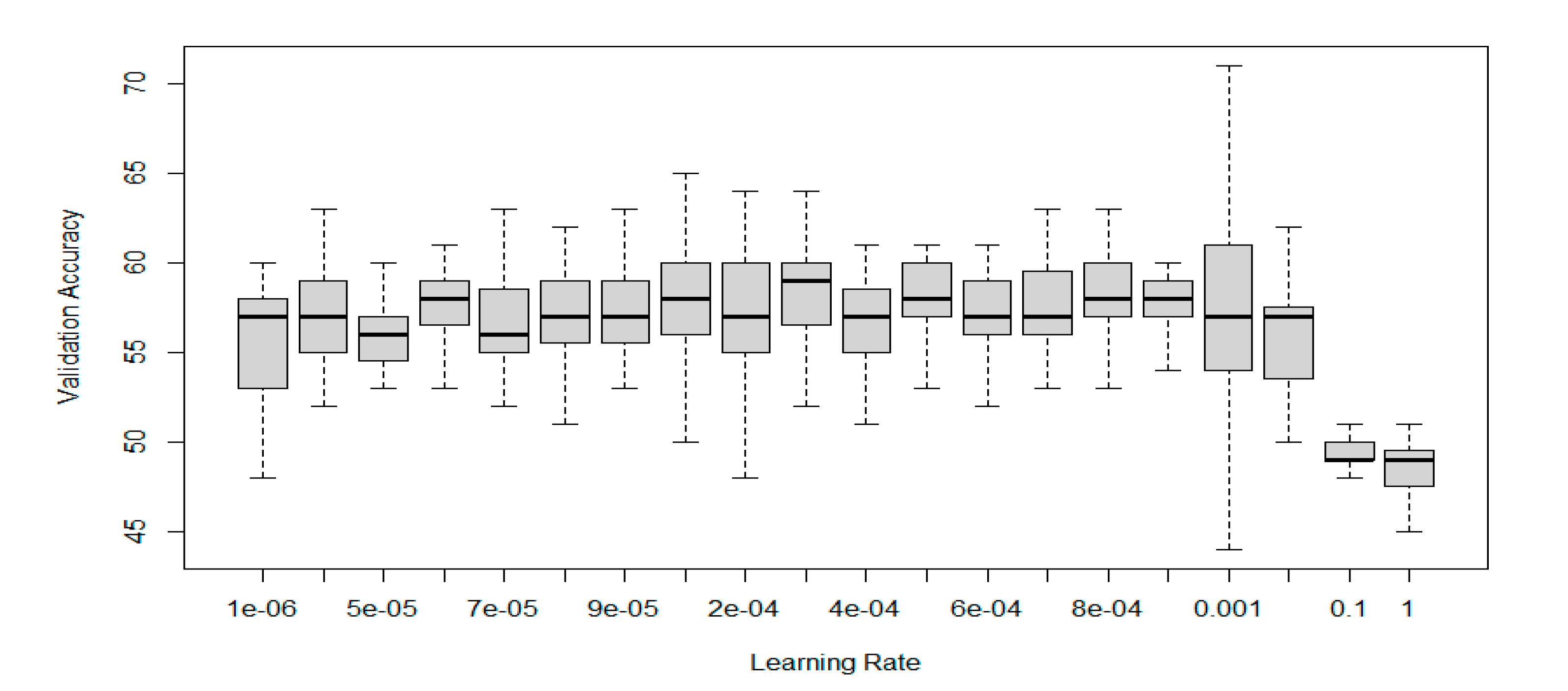
From the extent of the learning rate examination done during the study, a conclusion can be made, confirming information from the literature, stating a significant impact of this hyperparameter on the validation accuracy, as shown in
Figure 11.
Figure 11.
Effect of varying Learning Rate on the Validation Accuracy of Mixed Data classifiers.
Figure 11.
Effect of varying Learning Rate on the Validation Accuracy of Mixed Data classifiers.
Expectably, during the training and validation process, it was observed that the standard deviation correlated negatively with the number of training epochs. However, this standard deviation was not the smallest in the most accurate hyperparameters, as described in
Table 2,
Table 3 and
Table 4 and
Figure 8,
Figure 9 and
Figure 10. This effect is caused by the gradual generalisation of the trained models, leading to more stable performance and converging to a possible solution to the classification problem. However, the risk of using a larger number of training epochs is still related to the potential overfitting. It should be, therefore, adjusted temperately, considering the size of the training data set. A larger dataset allows for more epochs and a potentially improved validation or testing accuracy, as the model can learn from a more extensive variety of objects [
32]. Nevertheless, studies confirm that the training and classification work well even when using small datasets [
55,
56]. Mentioning the dataset size, it is necessary to mention that in this study, no test set was created, as it would be too small and imply statistical uncertainty, but it should be considered in future works, allowing for independent testing of trained classifiers.
As the classification of point clouds by the PointNet algorithm is not dependent on the orientation of the data or its resizing [
35], the dataset cannot be extended synthetically in a simple manner. Still, a slight randomisation or augmentation of the Point Cloud data was conducted even in the case of this study, allowing points to be slightly moved, by up to 5 mm, around their original position in the space. This may have caused changes in the accuracy of classifiers but may have also helped to generalise the model.
Some tree species may have similar properties of shape change after decaying, and combining such data into a single category might be helpful as it could provide more training data for each classifier and potentially improve classification accuracy. Unfortunately, in many cases, this is not true. The proposed study used three datasets containing various 3D meshes and tree species. The larger datasets in this study resulted in smaller validation accuracy, as it was made only by sorting the data by tree type – broadleaved or coniferous, respectively. The results confirm the presumption that creating a single classifier for each tree species is justifiable and results in more satisfying classification validation accuracy.
