Enhancing Tablet Dissolution Insights: A Comparative Study of Predictive ANN, PLS, and SVM Model With NIR Spectra

The pharmaceutical industry is making significant strides in enhancing process comprehension through the development of concepts like Quality by Design (QbD) and Process Analytical Technology (PAT). This shift has moved from traditional offline testing methods to real-time estimation of product quality. The dissolution characteristics of pharmaceutical tablets play a crucial role in maximizing the release of medications and their bioavailability. One factor that can affect dissolution is the blending procedure. Inadequate mixing can lead to patches of concentrated active components or excipients within the tablet, resulting in inconsistent dissolution behavior. A study investigated the impact of blending time and speed on the dissolution behavior of Amlodipine tablets using near-infrared (NIR) spectroscopy and multivariate modeling. NIR spectra were collected for Amlodipine tablets produced under various blending conditions using a 2-level central composite design. Dissolving profiles were analyzed using a USP dissolution device. Multivariate analysis techniques, including principal component analysis (PCA), partial least squares (PLS), Support Vector Machine (SVM), and Artificial Neural Networks (ANN), were applied to the collected NIR spectra. The findings demonstrated that blending speed and time had a significant influence on the dissolving properties of Amlodipine tablets. Blending at faster speeds and for shorter durations resulted in excessive shear and insufficient mixing, ultimately reduced drug release. The multivariate models constructed using ANN outperformed SVM and PLS in predicting dissolution profiles based on NIR spectra. This research highlights the effectiveness of NIR spectroscopy and multivariate modeling in optimizing tablet dissolution. These advancements enable continuous manufacturing of high-quality pharmaceutical products.

Keywords:

Subject: Medicine and Pharmacology - Pharmacy

1. Introduction

One of the sectors with the most regulations worldwide is the pharmaceutical one. Standards pertaining to drug efficacy and safety are crucial since this field produces goods that pose substantial danger to human health. The administration of medications in solid forms such as capsules and tablets are a prevalent and well-established practice in modern medicine. To maintain safety and efficacy, the manufacturing process includes frequent measurements of quality and process parameters. However, it’s impossible to understand every aspect that affects the drug’s quality, so in-process control measurements are necessary. Along with conventional batch manufacturing, Continuous manufacturing has also gained widespread acceptance. With the goal to assess and guarantee standard in both in-process and final products (CQAs), process management tools and observed materials characteristics of one or more (CQA) Critical Quality Attributes are integrated with RTRT. RTRT can help businesses to allocate resources more effectively, resulting in reduced laboratory costs and improved efficiency [1]. Real-time release testing (RTRT) is expressed as the process that can be used to replace some or all of the traditional end-product tests that are performed offline in order to verify that the drug product meets its quality specifications [2]. A Real-time release testing of dissolution focused on surrogate models constructed by algorithms based on machine learning utilizing NIR spectra, compression force and particle size distribution as input variables [3].

The RTRT idea is built on the Process Analytical Technology (PAT) Guideline framework. PAT uses in-line, online, or at-line analytical techniques to continuously monitor and adjust essential process parameters. PAT application and execution builds a powerful process monitoring and control in dosage form manufacturing [4]. Near-infrared spectroscopy (NIRS), which provides data in real-time despite a requirement for sample and is non-intrusive, is a suitable approach for this [5]. NIR spectroscopy has an extensive variety of applications, ranging from blending to evaluating and analyzing the finished dosage form e.g. identifying raw materials [6], examining the content uniformity [7] assessing particle size during the granulation process [8], moisture content [9], & assess the performance of coating operations [10].

The NIR spectra include an enormous amount of knowledge about a sample’s chemical and physical characteristics. To analyze the data, chemometric fundamentals, and multivariate models are used. Chemometrics applications include multivariate data evaluation and gathering processes, calibration, operation modelling, identification of patterns and categorization, signal improvement and compression, and statistical method management [11]. Following pre-processing of the data, multivariate models are constructed utilizing various techniques, including PCA (Principal Component Analysis) and PLS (Partial Least Squares), which are two of the most commonly used methods. The purpose of PCA is to compress the dimensionality of the spectra, while preserving a significant portion of its variation [12].

In addition to PLS models, other multivariate techniques such as neural networks (including artificial neural networks, or ANN) and support vector machines (SVM) are also commonly utilized in various fields for analyzing complex data. Artificial neural network (ANNs) is a form of computer technique created to mimic the brain’s capacity for interpreting data. Over the last several decades, ANNs have undergone substantial development it’s capacity to resolve multidimensional challenges with imperfect or obsolete data is a noteworthy benefit. [13]. Artificial neural networks (ANNs) are extensively utilized for determining the quantitative structure-activity relationship (QSAR) [14], as well as optimizing pharmaceutical formulations [15], and evaluating the dissolution pattern of pharmaceutical solid dosage forms [13]. Despite its numerous benefits, overfitting is a potential issue for ANN, which may restrict their usefulness. The Support Vector Machines (SVM) algorithm is one of the machine learning techniques applied for the categorizing, regression, and outlier recognition. Its main goal is to locate the optimum hyperplane in a high-dimensional space that can precisely distinguish between data points from various classifications [16]. It has been employed in meticulously identifying the raw materials [17], & for analyzing pharmaceutical drugs [18].

Dissolution test performance is an essential element of pharmaceutical drug manufacturing, evaluation, and analysis because it ensures that the medicines are safe and of superior quality for patients. Dissolution estimation helps in recognizing critical process parameters (CPPs) and developing dependable drug formulations that assure uniform and expected dissolution performance. Furthermore, dissolution prediction can aid in filings for regulatory approval and authorization by providing a scientific foundation for confirming the efficacy, safety, and quality of the drug [19]. Traditional dissolution methods destroy the tablet and render it unusable for further testing; however, advances in computational modelling as well as simulation techniques have made dissolution prediction more precise and valid, resulting in a rise in acceptance by the pharmaceutical sector. The study proposes a non-invasive NIR method for estimating dissolution profiles. This approach has a benefit over the current dissolution test, which renders the unit dose useless if it fails. The non-destructive NIR test can be used to investigate the cause of a unit’s failure using multivariate data analysis. Physical modifications in the drug substance or dosage as well as manufacturing process-related changes such as blending, coating, and compression force can also be detected using dissolution testing [13].

To achieve uniform tablet efficiency and dissolution, the API and excipients need to be blended uniformly. Inconsistent blending may result in a non-uniform dispersion of the ingredients, affecting the amount of dissolution and resulting in erratic tablet effectiveness. Thief sampling is commonly used to assess blend uniformity (BU). The powder characteristics influenced the evaluation as well as the thief geometry, such as the thief probe tip. It has been discovered that opting for a sample taken from the blender has an impact on evaluating the subsequent samples. Both systematic anomalies and the primary origin of fluctuations may come from this [20]. Size segmentation emerges from bed disruptions brought on by the introduction of the thieves [21,22]. Sacher and colleagues supplied a useful manual for PAT adoption for comprehensive process monitoring in the manufacture of solid dosages [23].

The present investigation employed the PAT methodology to examine how blending variables affect the dissolution of Amlodipine tablets. Using the Design of Experiments (DoE) strategy, the impact of blending time and speed on near-infrared (NIR) spectra was examined. The NIR data obtained, along with the dissolution test results, were used to develop chemometrics models such as Partial Least Squares (PLS), Support Vector Machines (SVM), and Artificial Neural Networks (ANN). Monitoring operational control data was critical for two reasons: 1) assessing blending variability and 2) predicting dissolution performance.

2. Materials and Methods

The active Ingredient used in this research is Amlodipine Besylate which is a calcium channel blocker and is a frequently recommended treatment. It is widely employed for the management of angina and hypertension. Amlodipine comes in the salt form of amlodipine besylate. It functions by preventing calcium ions from entering the smooth muscles of the heart and blood arteries. It assists in relaxing and enlarge the blood vessels by preventing calcium entrance, which lowers the pressure on the heart [24]. Amlodipine was used as the model medication because of its hygroscopicity and susceptibility to light. To investigate how NIR spectra affect these properties, NIR spectroscopy was employed. The research also sought to ascertain whether these characteristics affected the final formulation’s dissolution profile. For the tablet formulation, several raw materials were used from pharmaceutical grade vendor [25].

2.1. Blending:

All powdered ingredients were passed through sieves with 40 mesh openings per linear inch before introducing blending and lubrication, resulting in particles of consistent size and shape conducive to curtail the variation in dissolution profile due to irregular sized particles. The dissolution behavior of a tablet can be considerably impacted by the particles’ dimensions and shape in a powder blend. Smaller fragments with a greater surface area often dissolve more quickly, however irregularly shaped particles or ones having extended dispersion ranges are susceptible to decreased dissolution rates. Except for Magnesium Stearate, which was used as a lubricant, the API and other excipients were mixed together according to the formula. Blending time and speed were chosen during the pre-blending stage based on DoE runs according to the table presented above. In this experiment, Design Expert was employed to create Central Composite Design (CCD) with the factors blending time (X1) and blending speed (X2). The response variable is the dissolution rate (Y). The range was selected as 8 rpm to 16 rpm for blending speed and for blending time lower and upper values were 5 to 15 mins respectively. A total of 13 batches consisting of 9 batches with 5 center points repetitions were prepared. A factorial design featuring extra axial points and center points is used in the design, which enables the assessment of quadratic effects. Magnesium stearate has been mixed after the pre-blending and mixed for a duration of three minutes.

2.2. Tablet Compression:

Amlodipine Besylate immediate release tablets of strength 10 mg were prepared on a Rimek Minipress II at the ‘Department of Pharmaceutical Sciences, Dr. Vishwanath Karad, MIT World Peace University, Pune, India’. Concave Punches of 12mm were used. The ingredients were weighed manually on a calibrated Scale Tec balance (Model SAB-203) to ensure accuracy. The weighed ingredients were then added to the lower punch for compression, resulting in the production of tablets weighing 300 mg. 260 tablets were compressed, with each batch having 20 tablets. The compression force was kept constant at 0.75 tons throughout the compression process. On a calibrated balance, each tablet was carefully weighed, and any weight fluctuation was examined. It was found that all the tablets were within the stated weight limits, demonstrating the precision and accuracy of the weighing process.

2.3. NIR Scanning:

In this experiment, a NIR spectrometer made by Texas Instruments in Dallas, Texas was used to collect Diffuse Reflectance spectra. The spectrometer estimates the quantity of light that is reflected back from the material’s surface at various near-infrared wavelengths. The range used in this experiment was from 1700-900 nm, with a digital resolution of 447 nm and at an interval of 2 nm. The spectra were collected by placing a tablet in a glass petri dish at the centre of the NIR sensor. Ten scans were taken for each sample and averaged to five. The scan time for each tablet was 14.5 seconds. Before scanning the tablets, a white block was used as a reference material.

2.4. In-vitro Dissolution Testing:

Drug dissolution testing is conducted using a USP Paddle (Type II) apparatus having 500 ml of 0.01 M HCL as dissolution media and at 50 RPM in LabIndia (Model DS 8000, LabIndia pvt. Ltd, India) dissolution test apparatus. The temperature was set to 37±0.5°C. 10 tablets from each batch were subjected to a dissolution test and the test samples were extracted at every of 5, 10, 15, 20, and 30 mins. Subsequently, the aliquots were samples detected using a UV-VIS spectrophotometer (Shimadzu) and a wavelength of 239 nm [26]. The resultant absorbance was recorded and converted into the percentage of drug release which is further utilized for developing a calibrated model.

2.5. Multivariate Analysis:

NIR spectra commonly experience issues with undesired spectral variations and baseline shifts, which originate from a variety of sources. These include different types of noise produced by an amplifier, detector, as well as an AD converter, the scattering of light from opaque liquids or solid samples, alterations in sample temperature, along with its density, and particle size, inadequate reproducibility of NIR spectra due to factors like variations in path length, and baseline shifts resulting from the use of optical fiber cables. In order to avoid this noise in the spectra, different pre-processing parameters like Savitzsky-Golay Derivative, Smoothing, Standard Normal Variate (SNV), Multiplicative Signal Correction (MSC) are applied [27,28]. The Solo 9.2 demo version software from Eigenvector was used to analyze the NIR spectra. Pre-processing was necessary to obtain meaningful data from the spectral data, and the 1120-1620 nm range was chosen due to noisy signals outside this range. Principal component analysis (PCA) was employed to describe the patterns and evaluate how experimental conditions impacted the spectra. A PLS (Partial Least Squares) model was created using the principal components to generate latent variables through a linear combination of variables. An artificial neural network (ANN) model was built in MATLAB R2022 to anticipate the dissolution profile of the prepared tablets. The network’s efficiency was evaluated by altering the overall sum of neurons as long as 10 proved to be the ideal amount, then the hidden layer’s preferred number of neurons was determined. Finally, SVM (Support Vector Machine) regression models were constructed in Solo Eigenvector 9.2 demo version software using a radial basis function kernel, which is commonly used for nonlinear input-output relationships or when the input data lacks linear separability. Following any essential data preliminary processing, the model was developed. For further prediction, the NIR values from unknown test samples were added and the results for dissolution were predicted by comparing the behavior with the spectra. The NIR spectra here showed major shifts in the area of 1120 nm to 1620 nm range. The region before and after that contains lot of noise thus, for increasing the accuracy of model the region with significant spectral changes was selected from the whole spectra. These pre-processing parameters of all models are enlisted in the Table 1.

3. Results & Discussion

3.1. Principal Component Analysis (PCA)

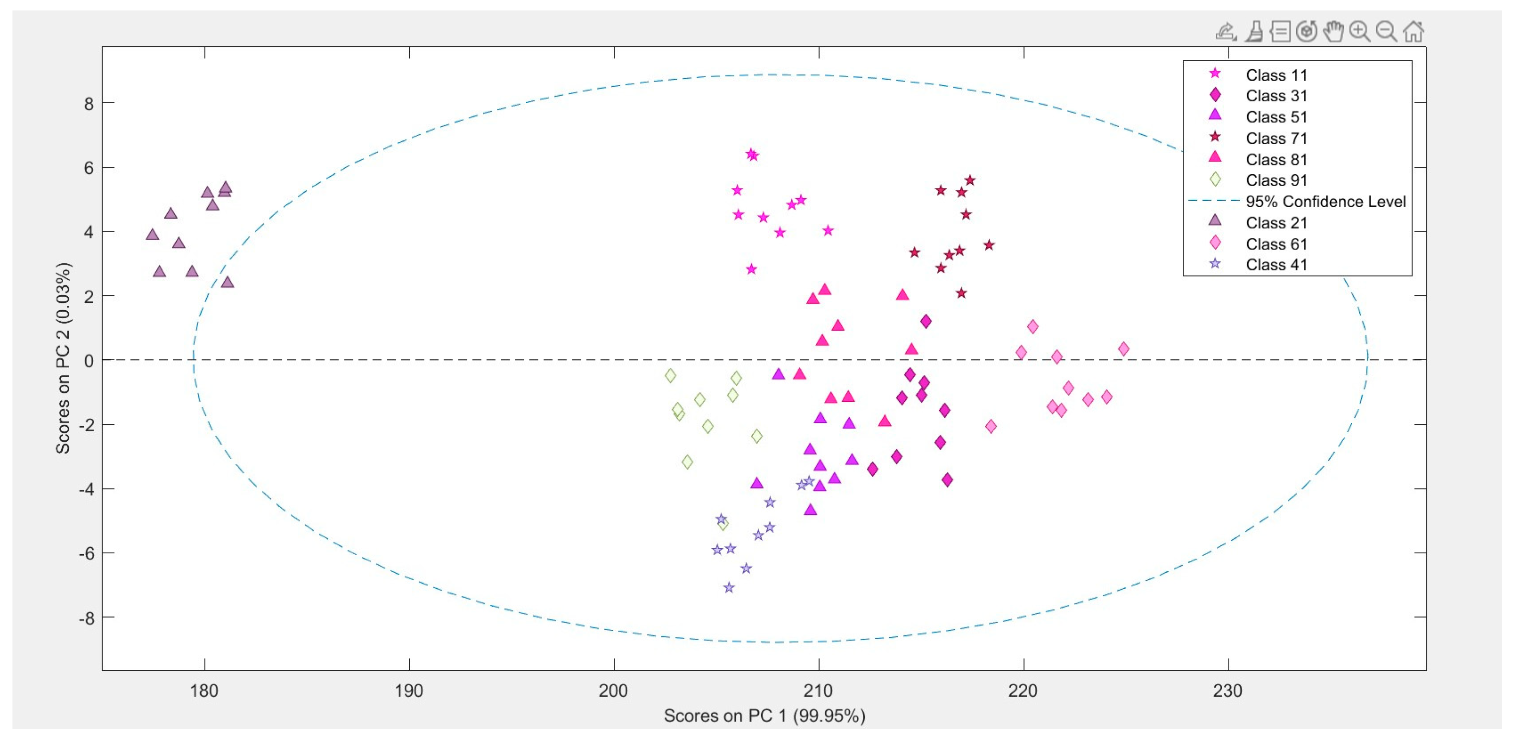
Principal Component Analysis (PCA) is a technique that can be used to extract the most significant features in a dataset and explain its variability. PCA clarifies the dataset’s data variation and assists in dividing the data into the principal components that accurately describe the data. This enables the separation of data into the primary components that best describe the data. Several pre-treatment parameters were used to further resolve and sharpen the variation peak from overlapping spectras, including Savitzky-Golay (SG) 2nd order derivative fitted with 3 Smoothing points subsequent to that, Standard Normal Derivative (SNV). The Savitzky-Golay filter was used to get a signal’s second-order derivative. It can also be employed to classify data. It is especially helpful for dealing with noisy data. Smoothing (up to 3 points) to further enhance spectral resolution, and the features were adjusted to an appropriate range through normalization via Standard Normal Variate (SNV). The PCA method was used to decompose the data related to drug release in this case. The principal components can be calculated using a variety of techniques. These are typically computed using the data matrix’s mean-cantered covariance matrix. The singular value decomposition (SVD) technique was created on the basis of the notion that a set of values can be expressed as a combination of three specific matrices. The PCA model with two principal components, which could account for 99.96% of the variation, was chosen. As can be seen, PC 1 was able to account for 99.91% of the variance in the data, whereas PC 2 accounted for the final 0.5%. For the purpose of cross validation, Venetian blinds w/ 10 splits and blind thickness = 1 was utilized with SVD algorithm.

According to the Figure 1, the batches are distributed along a range of blending speeds, with batches 2 and 6 located at the two extremes of the distribution. The bleeding rpm in batch 2 was the highest, while the rpm in batch 6 was the lowest. The remaining batches were situated between these two extremes. Based on this data, it can be deduced that when the blending speed exceeds a certain threshold, the percentage of drug released during dissolution decreases. As a result, the rate of drug dissolution and blending speed are inversely related.

It was critical to eliminate any systematic variation in the data caused by differences in the average values of the variables before analyzing the dependent variables measured at different time intervals of 5, 10, 15, 20, and 30 minutes in the dissolution test. The data were mean-centered to achieve this. This step is critical because it allows the variables’ relative values to be more important than their absolute values. It also aids in the accurate identification of variable relationships. Following the mean-centering process, a model was built to further analyze the data. The model’s statistical parameters are as follows (Table 2):

3.2. Partial Least Squares (PLS):

For the purpose of predicting the drug release profile, a Partial Least Squares (PLS) model was implemented with the decomposed data from PCA. The response variable was the percentage of drug release from the same ten tablets, and the predictors for the PLS model were the averaged Near Infrared (NIR) spectra of ten tablets from every batch of tablets. Mean cantering was utilized as a pre-processing method to eliminate any offset, which also increased the model’s readability and precision. The response variables which are the dependent factors in the dissolution test are investigated at various time intervals of 5 to 30 minutes. The data was mean-cantered to exclude systematic error in the data that results from variations in the mean of the variables. This is vital since systematic variation can make it difficult to identify correlations between variables accurately and therefore the relative values of the variables are frequently more important than their absolute values. The starting manifestation variables are linearly combined to create the latent variables produced by the PLS regression. The implications of each latent variable were examined in order to understand the reasons of variability. The 1st latent variable accounted for 36.26% of the overall variation. A model with 5 latent variables was showing less RMSE values and thus, it was chosen. After all, the model was built, and its statistical settings are represented in Table 2.

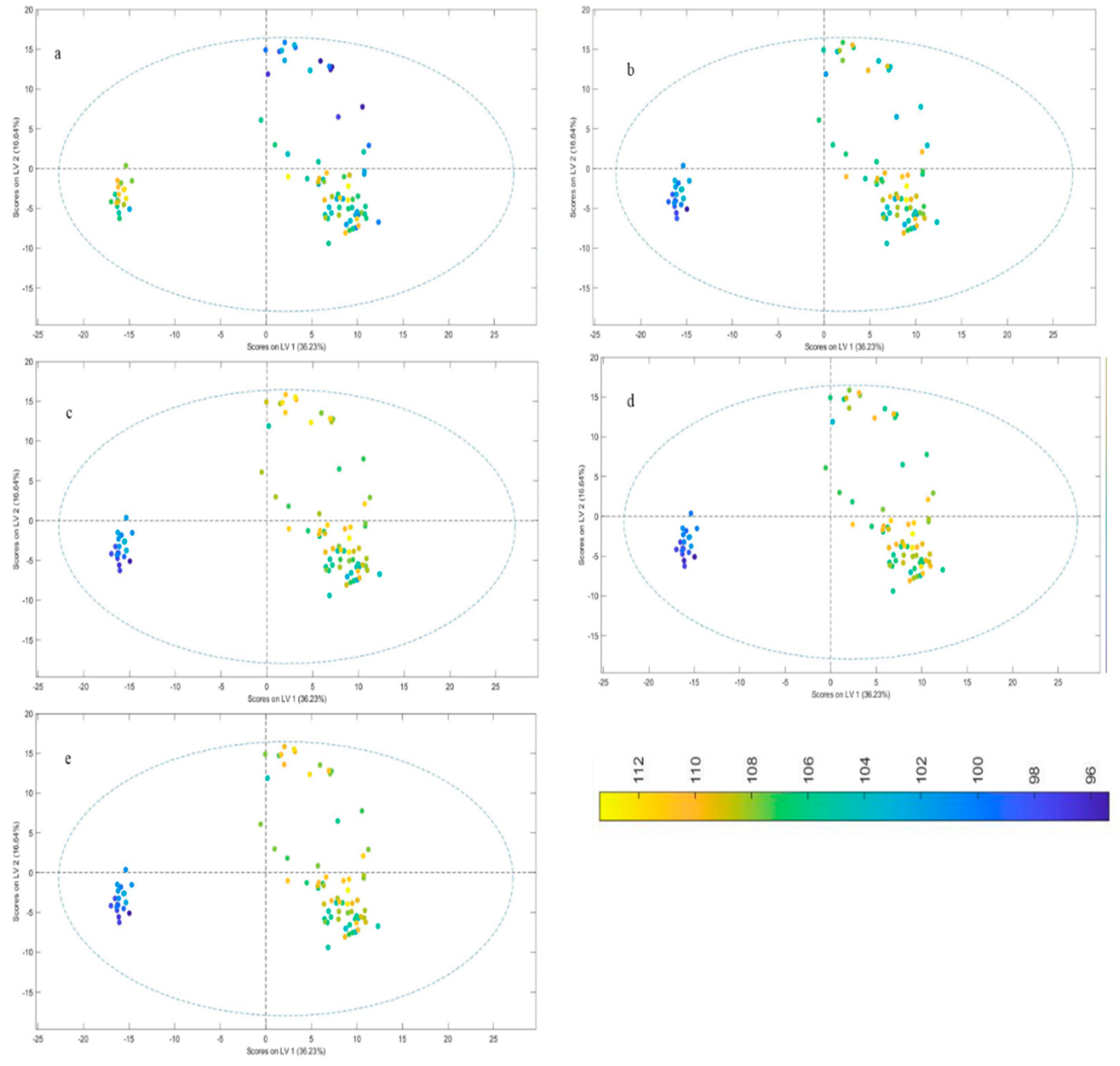
The clusters in the score plot (Figure 2) have been categorized in accordance with the varied blending speed and time, and the legend in the image depicts the release of the drug at various time intervals. The amount of medication released from tablets manufactured under various blending circumstances was seen to vary noticeably. The maximum drug release did not exceed 100% in runs 2 and 3, which had the highest blending RPM and lowest blending time, respectively, according to the observed data, which clearly show that differences in the blending combinations have a substantial influence on the release of the medicine.

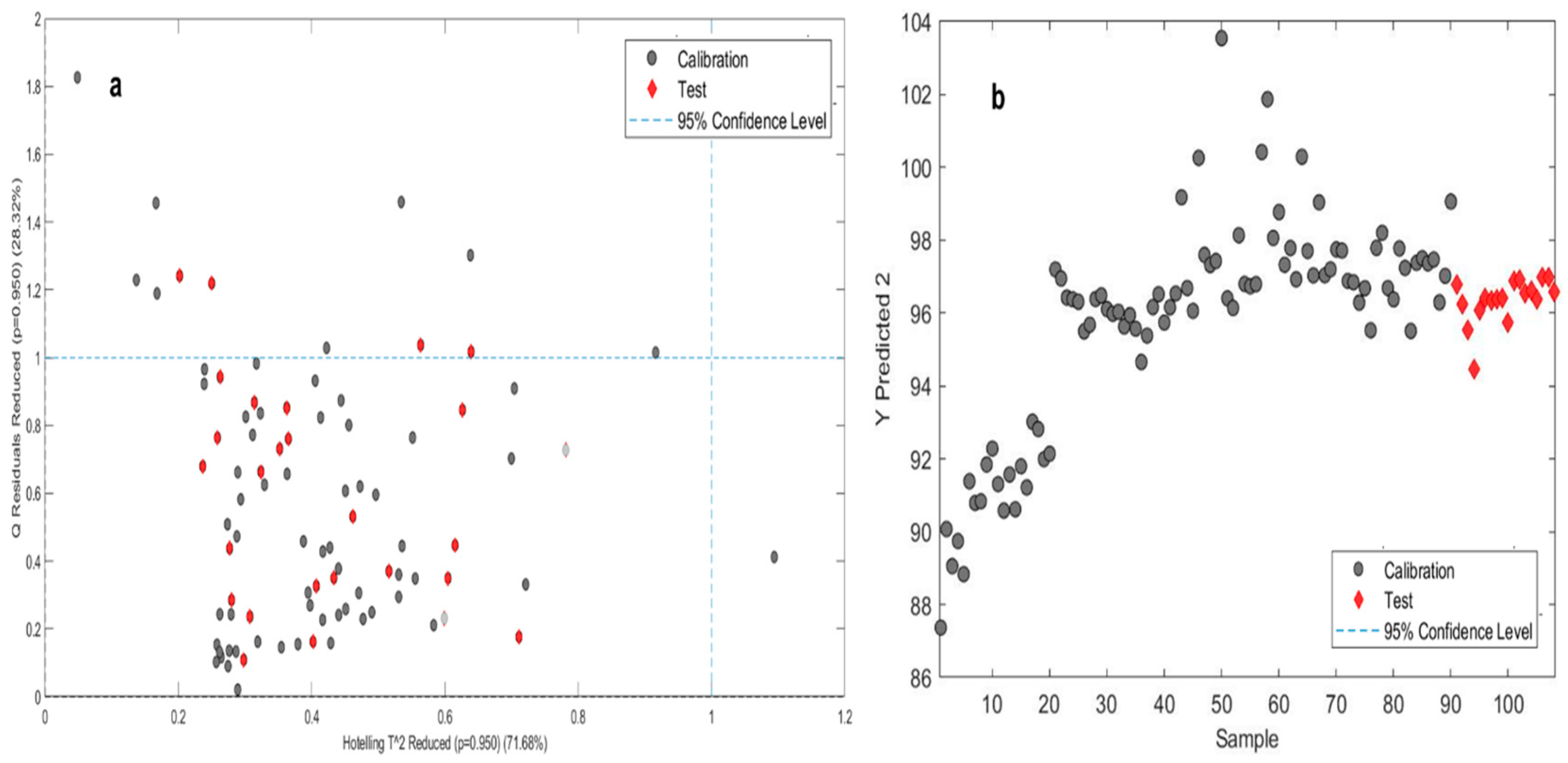
A combined total of 18 tablets, two from each batch, were chosen for validating the model. In the dissolution prediction approach, the calibration model with the lowest root mean square (RMS) value was employed. Relevant pre-processing approaches were used to calibrate the selected model and the resulting dissolution profile was satisfactory. A graph depicts the predicted dissolution profile. To validate the model, the partial least squares (PLS) model was implemented to a completely separate validation set’s near-infrared (NIR) spectra. The PLS model estimates the % of drug release at specific time points accurately, and the PLS score plots demonstrate clear separation of the validation samples, similar to the calibration set samples. When the predicted release profile values were compared to the actual measured release profile, it was observed that they were both within the specified limits. A graph (Figure 3) demonstrates the connection between the validation and calibration datasets, with the validation set marked by red dots and the calibration set represented by grey dots. The results of the validation set were found to be within the limits of the calibrated dataset. Afterwards the model’s validation, an unknown dataset consisting of two tablets from each batch was chosen, and the dissolving profile of those tablets was subsequently estimated applying the built-in model. The generated calibration model and the model utilized for prediction shared the same statistical attributes.

3.3. Support Vector Machine (SVM):

Using the Epsilon-SVR approach, a machine learning model called support vector machine was created. For the sake of improving the accuracy and validity, the model analyzed the data with a radial basis function kernel. Various signal processing strategies were implemented to the spectra in order to minimize noise while enhancing the overall quality of the data. To begin, the Automatic Whittaker Filter and second-order derivative were used to correct the baseline. The spectra were then normalized using Multiplicative signal correction to remove unwanted scattering effects. Finally, the spectra were resolved using Standard Normal Variance (SNV). These techniques were successful in reducing noise and improving data analysis accuracy. The dissolution time intervals of 5, 10, 15, 20, and 30 were selected as Y columns 1 to 5 respectively. Statistical parameters of the SVM model are represented in the table 2.

3.4. Artificial Neural Network (ANN):

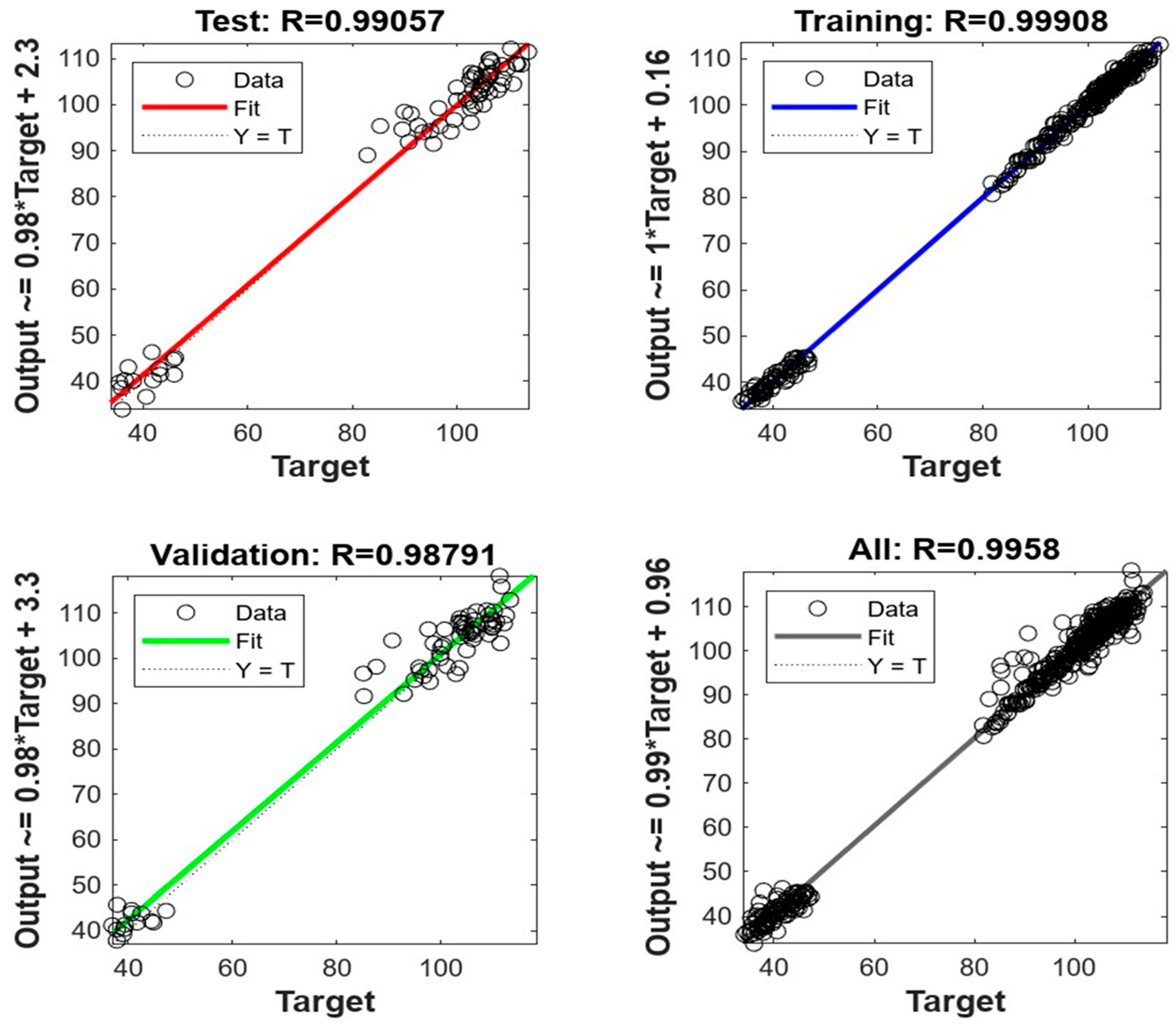
MATLAB software from Mathworks, Inc. in the United States was used to develop a model for an artificial neural network (ANN). The Levenberg-Marquardt Algorithm was adopted for learning the model, which included ten layers. The data was split into three groups: training data (70%), validation data (15%), and test data (15%) in order to assess the effectiveness of the model. The table 2 presents the model’s statistics metrics. The data was found to in line with the inclination line of fit. The R values were found to be 0.9991, 0.9879, 0.9906, and 0.9958 for training, validation, test, and overall model (Figure 4). This shows that the ANN model has a good potential in predicting the dissolution profiles of further tablets.

3.5. Prediction of Dissolution Profile:

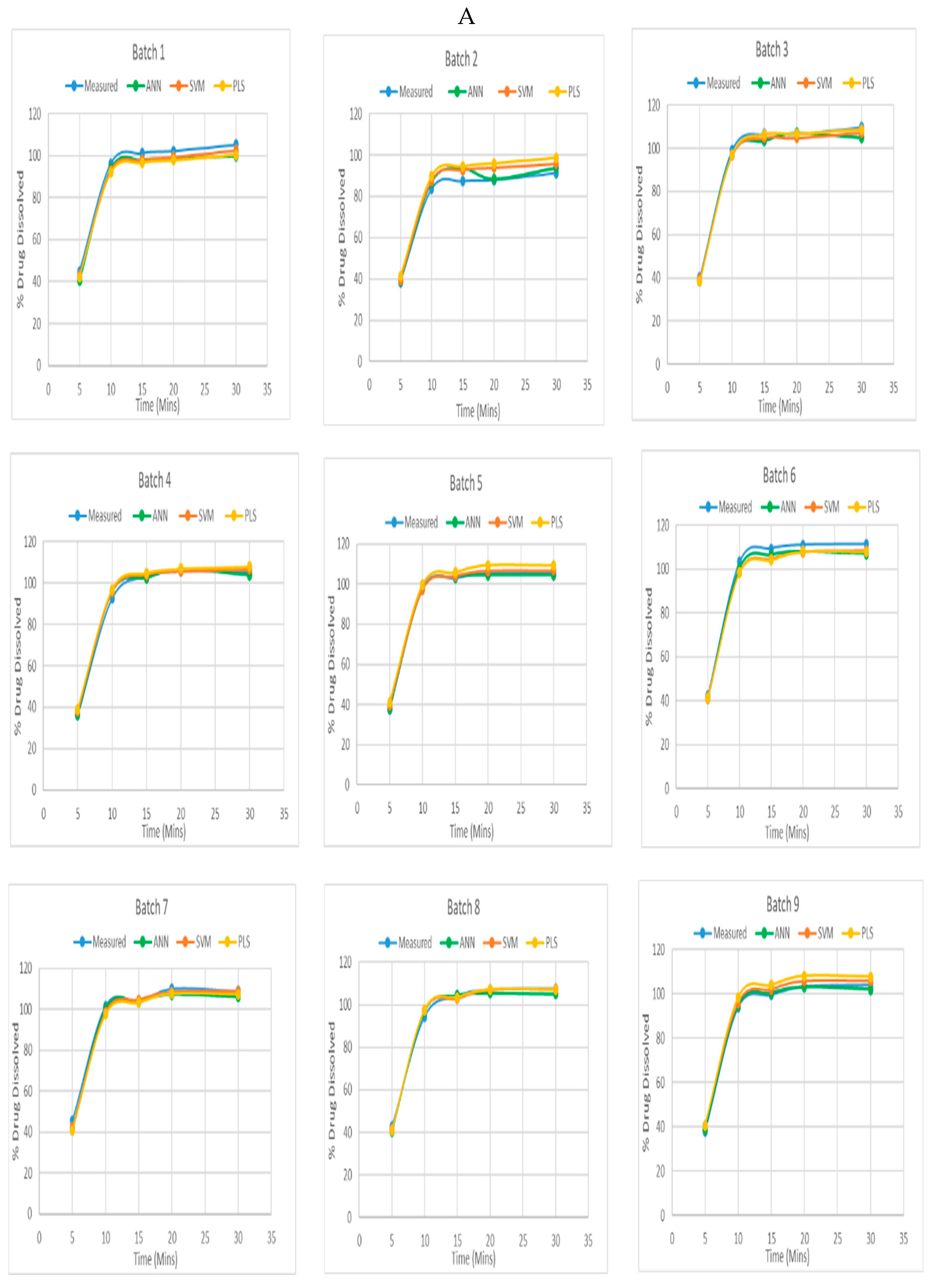
The NIR spectrum of the amlodipine tablets and the dissolution tests data at time intervals of 5, 10, 15, 20, and 30 minutes were the inputs for each multivariate model. Additionally, the proper pre-processing methods were used, and a calibrated model was constructed. Plotting and comparing the results of the dissolution profile that were obtained resulting from the dissolution studies with the predicted outcomes of the models. Out of total 13 experimental runs which were generated after constructing the design, had 5 central points and the rest being either axial or factorial points. Thus, the prediction graph of one representative of central run and other axial and factorial runs were plotted. The following are the graphs for each batch. (Figure 5 A)

The disparities in the generated models’ performance might be attributed to the intricacy of the models, the extent of the dataset, and the features used to train them. Other reason might be the models’ various operational approaches that are most likely what causes the variation in accuracy amongst them. Artificial neural network has mastered the ability to decipher complicated patterns in data. The SVM models, which are classified as support vector machines, have the capacity to identify the best hyperplanes for dividing two different data classes. PLS models, on the other hand, are categorized as partial least squares regression, which successfully enables them to identify linear combinations of factors that predict response variables with a high level of accuracy. 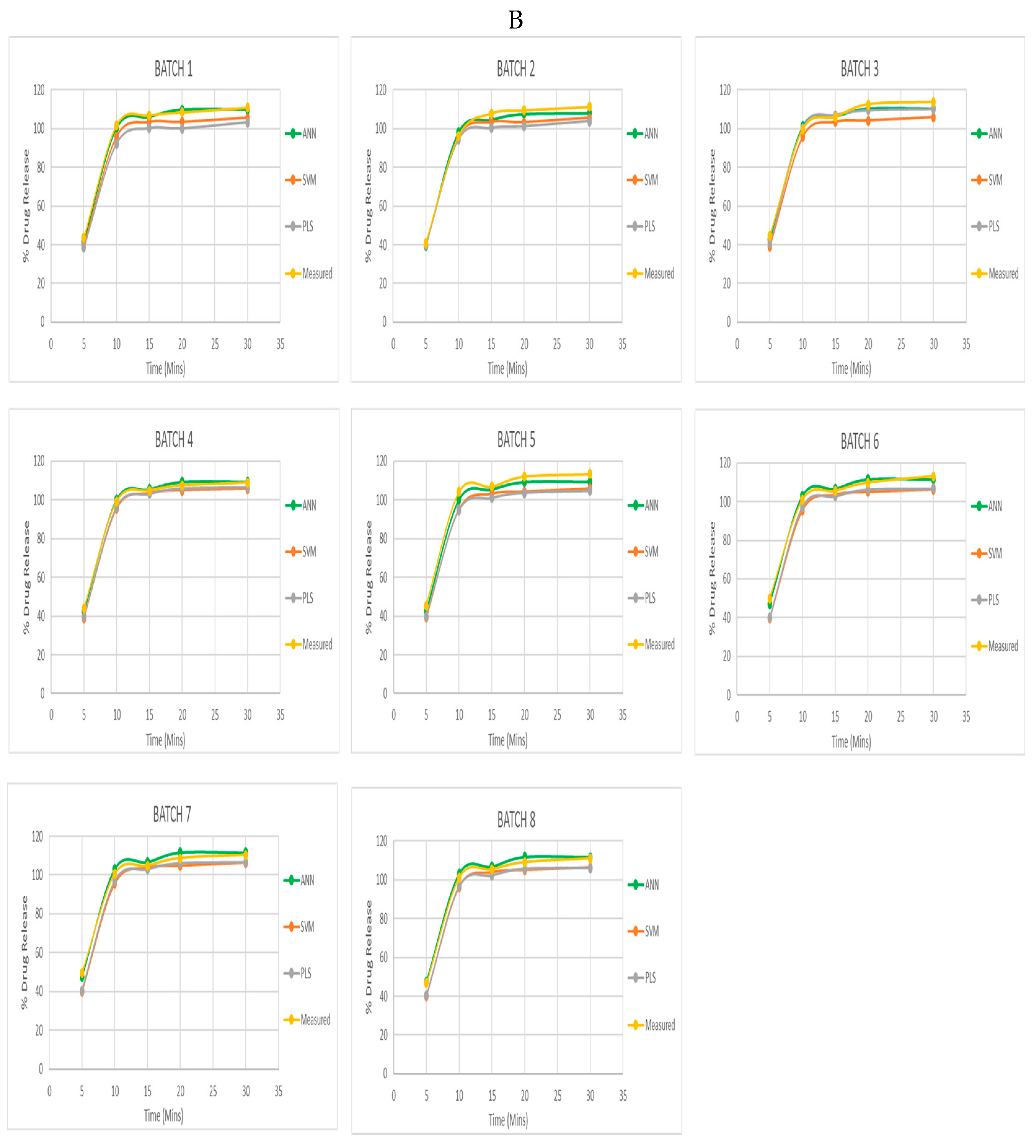The graph (Figure 5 B) above represents calibration graphs of PLS, SVM, and ANN are plotted against the actual drug release of all 9 batches. Once validated and calibrated, the dissolution pattern of an unidentified set of tablets has been predicted using the model. The results were presented in a graph after using two tablets with unknown parameters for the unknown dataset. For this, the NIR spectra of the unidentified amlodipine tablets were integrated to the models that had already been created. This calibrated model was then used to forecast the results and the graph displayed the dissolution profile of the tablets over time (Figure 5 B). In the Figure 5 B The graphs demonstrate that the multivariate models created were capable of accurately predicting the dissolution profile of the produced Amlodipine tablets. The dissolution pattern was possibly predicted with a high degree of accuracy using ANN models, and the values expected were very close to the measured values. The ANN models were better at closely matching the measured values than the SVM models at predicting the dissolution profile with high accuracy. The PLS model was the least accurate of the three since the predicted and measured values were substantially diverging.

3.6. Model Independent Approach for F1 and F2 Calculation:

A model-independent approach to dissolution testing involves analyzing experimental dissolution profiles without assuming a specific kinetic model. This method makes it possible to compare dissolution profiles between various goods without having to rely on a single kinetic model, which is especially helpful for dissolving processes or profiles that are complex or unfamiliar or don’t adhere to a particular kinetic model. Moore and Flanner proposed a straightforward model-free method in 1990 that involves estimating two variables, the similarity factor (F2) and the difference factor (F1). Use the following formulas to determine F1 and F2:

F1 = 100 x Σ|C_ref - C_test| / ΣC_ref

(1)

F2 = 50 x log {[Σ(t=1 to n) (R_t - T_t)^2] / [Σ(t=1 to n) R_t^2 + Σ(t=1 to n) T_t^2]}

(2)

Where, the cumulative % dissolved of the reference product at each time point, denoted as C_ref, and the cumulative % dissolved of the test product at each time point, denoted as C_test. The F2 formula involves using the percentage dissolved of the reference product at each time interval, represented by R_t, and the percentage dissolved of the test product at each time period, represented by T_t. The formula is calculated for a total of n time points.

When the value is zero, the two profiles are equal, while rising values signify greater disparities. The dissolution profiles are regarded as equal if the F1 value is less than 15, and F2 value within the range of 50 to 100, according to statistics [29].

3.7. Model Dependent Approach for F1 and F2 Calculation:

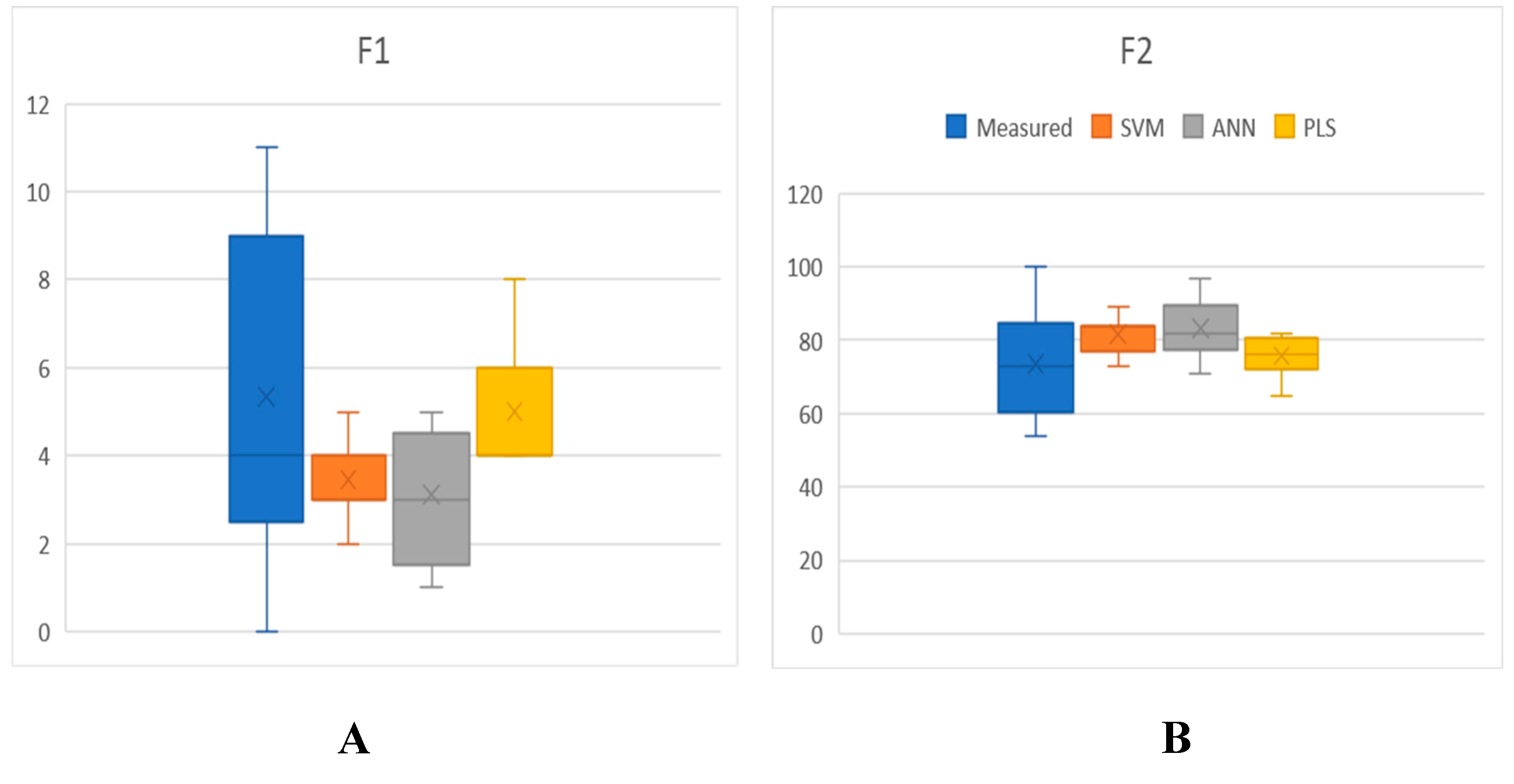
The box-plots in Figure 6 illustrate the distribution of F1 and F2 values computed across all measured tablets and PLS, SVM, and ANN models. The y-axis depicts the magnitude of F1 and F2 values, while the x-axis represents the three data sets. The figure emphasizes the range and asymmetry of the data distribution. For every model, the box-plot displays its median, mean, 25th, and 75th quartiles, as well as the range of nine F1 and F2 values and outliers. The findings indicate that the majority of models had a mean F1 score below 4, but a mean F2 score above 79, which suggests that their predictive accuracy could satisfy the necessary level of authority standards.

5. Conclusions

To establish the optimal drug delivery, tablet manufacturing is a complex process that calls for meticulous evaluation of numerous parameters. In the present research, we explored at how blending time and speed impacted the dissolution profile of tablets containing amlodipine, a medication frequently prescribed for angina and hypertension. Our research showed that both blending duration and speed had a substantial effect on the dissolution profile, with blending speed having a far greater detrimental effect on the drug’s dissolution. This emphasizes how critical it is to precisely regulate the blending speed throughout the production process in order to get the proper dissolution profile for Amlodipine tablets. Consequently, if these variables were under control, desired quality might be attained.

To investigate the dissolution profile, we used near-infrared (NIR) spectra to record data, which we then used to create multivariate models such as partial least squares (PLS), artificial neural networks (ANN), and support vector machines (SVM). The results indicated that the ANN models demonstrated greater accuracy and similarity to the measured F2 and F1 values, followed by the SVM models, and lastly, the PLS models.

This suggests that ANN models may be more practical and dependable for measuring F2 and F1 values in comparison to the other two models. Thus, the ANN was the most accurate model in predicting the dissolution profile, followed by SVM and then PLS. This shows that machine learning models have great potential for predicting the dissolution profile of tablets and optimizing the formulation step. The results of our study may have important implications for pharmaceutical manufacturing, as they provide valuable insights into the factors that influence the dissolution profile of tablets. By carefully controlling blending speed, pharmaceutical companies may be capable to monitor and optimize the formulation process of Amlodipine tablets to achieve the desired dissolution profile. In conclusion, our study highlights the importance of considering various factors during the manufacturing process of tablets and the potential benefits of using machine learning models for predicting dissolution profiles.

Author Contributions

“Conceptualization, Shruti Ringe and Abhijeet Sutar; methodology, Shruti Ringe and Shounak Kulkarni; software, Suresh Kumar BV and Anurag Shenoy; validation, Shruti Ringe, Shounak Kulkarni and Abhijeet Sutar.; formal analysis, Shruti Ringe and Shounak Kulkarni; investigation, Shruti Ringe and Shounak Kulkarni; resources, Shruti Ringe, Shounak Kulkarni, Abhijeet Sutar, Suresh Kumar BV, and Anurag Shenoy ; data curation, Shruti Ringe and Shounak Kulkarni; writing—original draft preparation, Shruti Ringe; writing—review and editing, Shruti Ringe and Abhijeet Sutar; visualization, Shruti Ringe, Shounak Kulkarni and Abhijeet Sutar; supervision, Abhijeet Sutar and Suresh Kumar BV; project administration, Abhijeet Sutar; All authors have read and agreed to the published version of the manuscript.”.

Funding

This research received no external funding.

Institutional Review Board Statement

“Not applicable”.

Informed Consent Statement

“Not applicable.”.

Data Availability Statement

The data presented in this study are available on request from the corresponding author. The data are not publicly available due to [Privacy].

Acknowledgments

We acknowledge the invaluable support from Dr. Vishwanath Karad MIT World Peace University, School of Health Science and Technology, and Elico Healthcare Services, who provided essential research facilities. We also extend our appreciation to Elico Healthcare Services for the use of the NIR spectrometer, which greatly enhanced the precision of our experiments.

Conflicts of Interest

“The authors declare no conflict of interest.” “The funders had no role in the design of the study; in the collection, analyses, or interpretation of data; in the writing of the manuscript; or in the decision to publish the results”.

References

Pawar, P. Tools for real time release testing (RTRt) in batch and continuous tablet manufacturing. Rutgers The State University of New Jersey, School of Graduate Studies; 2016.
Markl, D.; Warman, M.; Dumarey, M.; Bergman, E.L.; Folestad, S.; Shi, Z.; Zeitler, J.A. Review of real-time release testing of pharmaceutical tablets: State-of-the art, challenges and future perspective. Int. J. Pharm. 2020, 582, 119353. [Google Scholar] [CrossRef]
Galata, D.L.; Könyves, Z.; Nagy, B.; Novák, M.; Mészáros, L.A.; Szabó, E; Nagy, Z.K. Real-time release testing of dissolution based on surrogate models developed by machine learning algorithms using NIR spectra, compression force and particle size distribution as input data. Int. J. Pharm. 2021, 597, 120338. [Google Scholar] [CrossRef] [PubMed]
Sacher, S.; Poms, J.; Rehrl, J.; Khinast, J.G. PAT implementation for advanced process control in solid dosage manufacturing – A practical guide. Int. J. Pharm. 2022, 613, 121408. [Google Scholar] [CrossRef] [PubMed]
Pestieau, A.; Krier, F.; Thoorens, G.; Dupont, A.; Chavez, P.F.; Ziemons, E.; Evrard, B. Towards a real time release approach for manufacturing tablets using NIR spectroscopy. Journal of Pharmaceutical and Biomedical Analysis 2014, 98, 60–67. [Google Scholar] [CrossRef]
Zhang, Y.; Cheng, Q.; Chang, C.; Zhang, L. Phase transition identification of cellulose nanocrystal suspensions derived from various raw materials. J. Appl. Polym. Sci. 2017, 135, 45702. [Google Scholar] [CrossRef]
Blanco, M.; Alcalá, M. Content uniformity and tablet hardness testing of intact pharmaceutical tablets by near infrared spectroscopy. Anal. Chim. Acta 2006, 557, 353–359. [Google Scholar] [CrossRef]
Pauli, V.; Roggo, Y.; Kleinebudde, P.; Krumme, M. Real-time monitoring of particle size distribution in a continuous granulation and drying process by near infrared spectroscopy. Eur. J. Pharm. Biopharm. 2019, 141, 90–99. [Google Scholar] [CrossRef]
Duthen, S.; Levasseur-Garcia, C.; Kleiber, D.; Violleau, F.; Vaca-Garcia, C.; Tsuchikawa, S.; Daydé, J. Using near-infrared spectroscopy to determine moisture content, gel strength, and viscosity of gelatin. Food Hydrocoll. 2021, 115, 106627. [Google Scholar] [CrossRef]
Tabasi, S.H.; Fahmy, R.; Bensley, D.; O’Brien, C.; Hoag, S.W. Quality by Design, Part II: Application of NIR Spectroscopy to Monitor the Coating Process for a Pharmaceutical Sustained Release Product. J. Pharm. Sci. 2008, 97, 4052–4066. [Google Scholar] [CrossRef]
Chemometrics in Environmental Chemistry - Statistical Methods (Vol. 2 / 2G). Einax, J.; Einax, J. (Eds.) 2013. [Google Scholar]
Kumar, K. Partial least square (PLS) analysis: Most favorite tool in chemometrics to build a calibration model. Resonance 2021, 26, 429–442. [Google Scholar] [CrossRef]
Nagy, B.; Petra, D.; Galata, D.L.; Démuth, B.; Borbás, E.; Marosi, G.; Farkas, A. Application of artificial neural networks for Process Analytical Technology-based dissolution testing. Int. J. Pharm. 2019, 567, 118464. [Google Scholar] [CrossRef]
Montañez-Godínez, N.; Martínez-Olguín, A.C.; Deeb, O.; Garduño-Juárez, R.; Ramírez-Galicia, G. QSAR/QSPR as an application of artificial neural networks. Methods in Molecular Biology (Clifton, N.J.), 2015, 1260, 319–333. [Google Scholar] [CrossRef]
Ibrić, S.; Djuriš, J.; Parojčić, J.; Djurić, Z. Artificial Neural Networks in Evaluation and Optimization of Modified Release Solid Dosage Forms. Pharmaceutics 2012, 4, 531–550. [Google Scholar] [CrossRef]
Gholami, R.; Fakhari, N. Support Vector Machine: Principles, Parameters, and Applications. Handbook of Neural Computation 2017, 515–535. [CrossRef]
Sun, L.; Hsiung, C.; Pederson, C.G.; Zou, P.; Smith, V.; von Gunten, M.; O’Brien, N.A. Pharmaceutical Raw Material Identification Using Miniature Near-Infrared (MicroNIR) Spectroscopy and Supervised Pattern Recognition Using Support Vector Machine. Appl. Spectrosc. 2016, 70, 816–825. [Google Scholar] [CrossRef]
Burbidge, R.; Trotter, M.; Buxton, B.; Holden, S. Drug design by machine learning: support vector machines for pharmaceutical data analysis. Comput. Chem. 2001, 26, 5–14. [Google Scholar] [CrossRef]
Lee, S.L.; Raw, A.S.; Yu, L. Dissolution Testing. Biopharmaceutics Applications in Drug Development. 2008, 47–74. [Google Scholar] [CrossRef]
Harwood, C. F.; Ripley, T. Errors associated with the thief probe for bulk powder sampling. J. Powder Bulk Solids Technol. 1977, 11, 20–29. [Google Scholar]
Muzzio, F.J.; Alexander, A.; Goodridge, C.; Shen, E.; Shinbrot, T.; Manjunath, K.; Jacob, K. (n.d.). Solids Mixing. Handbook of Industrial Mixing, 887–985. [CrossRef]
Velez, N.L.; Drennen, J.K.; Anderson, C.A. Challenges, opportunities and recent advances in near infrared spectroscopy applications for monitoring blend uniformity in the continuous manufacturing of solid oral dosage forms. Int. J. Pharm. 2022, 615, 121462. [Google Scholar] [CrossRef]
Sacher, S.; Poms, J.; Rehrl, J.; Khinast, J.G. PAT implementation for advanced process control in solid dosage manufacturing – A practical guide. Int. J. Pharm. 2022, 613, 121408. [Google Scholar] [CrossRef]
Murdoch, D.; Heel, R.C. Amlodipine. Drugs 1991, 41, 478–505. [Google Scholar] [CrossRef]
Amlodipine Besylate Tablets. United States Pharmacopoeia, (2011). Uspnf.com website: https://www.uspnf.com/sites/default/files/usp_pdf/EN/USPNF/amlodipineBesylateTabletsm3575 Accessed 15 Sept 2022.
USP, 2011. Available online: https://www.uspnf.com/sites/default/files/usp_pdf/EN/USPNF/amlodipineBesylateTabletsm3575.pdf. Accessed 12 Sept 2022.
Martens, H.M.A.M. Multivariate Analysis of Quality. An Introduction. Meas. Sci. Technol. 2001, 12, 1746–1746. [Google Scholar] [CrossRef]
Near-Infrared Spectroscopy. Siesler, H.W.; Ozaki, Y.; Kawata, S.; Heise, H.M. (Eds.) 2001. [Google Scholar] [CrossRef]
Saranadasa, H.; Krishnamoorthy, K. A Multivariate Test for Similarity of Two Dissolution Profiles. J. Biopharm. Stat. 2005, 15, 265–278. [Google Scholar] [CrossRef] [PubMed]

Figure 1. PCA plot explaining clustering of batches.

Figure 2. PLS Score plots showing release at different time points. (a)- Release at 5 mins. (b)- Release at 10 mins. (c)-Release at 15 mins. (d)- Release at 20 mins. (e)- Release at 30 mins.

Figure 3. Loading plots for Validation set and test samples. (a)- Validation set. (b)- Test set.

Figure 4. Test, Validation, Training and the overall graphs for ANN.

Figure 5. A: Calibration graphs of Measured, PLS, SVM, and ANN from batch 1 to 9. B: Average of the predicted and the measured dissolution profiles by PLS, SVM and ANN.

Figure 6. Box-Whisker plots for A. F1 and B. F2 values of Measured, PLS, SVM and ANN.

Table 1. NIR pre-processing parameters.

Method	Pre-processing Parameters
Region Selection	1120 nm to 1620 nm
PCA	1st Derivative for decomposition
PLS	2nd Derivative (order: 2, window: 15 pt, tails: polyinterp), Smoothing (order: 0, window: 3 pt, tails: polyinterp), SNV
SVM	Baseline (Automatic Whittaker Filter, asymmetry=0.001 lambda=100), 2nd Derivative (order: 2, window: 15 pt, tails: polyinterp), Smoothing (order: 0, window: 7 pt, tails: polyinterp), MSC (Mean), SNV
ANN	10 neurons

Table 2. Statistical Parameters of PCA, PLS, SVM, & ANN model.

Statistical Parameters	Time Points	RMSEC	RMSECV	R² CAL	R²CV
PCA	nil	1.429	3.241	nil	nil
PLS	5 mins	3.158	3.567	0.175	0.026
	10 mins	3.768	4.595	0.535	0.328
	15 mins	3.556	4.175	0.627	0.492
	20 mins	3.615	4.337	0.671	0.533
	30 mins	3.495	4.18	0.693	0.529
SVM	5 mins	0.742	2.786	0.962	0.351
	10 mins	0.956	4.152	0.98	0.454
	15 mins	1.271	3.91	0.959	0.568
	20 mins	0.915	3.798	0.982	0.658
	30 mins	0.01	3.441	0.999	0.626
ANN	Training	1.084	nil	0.9991	nil
	Validation	4.163	nil	0.9879	nil
	Test	3.509	nil	0.9906	nil

RMSEC- Root Mean square error of calibration; RMSECV- Root Mean Square Error of Cross Validation; R2 CAL- R2 Calibration; R2 CV- R2 Cross Validation.

Disclaimer/Publisher’s Note: The statements, opinions and data contained in all publications are solely those of the individual author(s) and contributor(s) and not of MDPI and/or the editor(s). MDPI and/or the editor(s) disclaim responsibility for any injury to people or property resulting from any ideas, methods, instructions or products referred to in the content.

© 2023 by the authors. Licensee MDPI, Basel, Switzerland. This article is an open access article distributed under the terms and conditions of the Creative Commons Attribution (CC BY) license (http://creativecommons.org/licenses/by/4.0/).

Copyright: This open access article is published under a Creative Commons CC BY 4.0 license, which permit the free download, distribution, and reuse, provided that the author and preprint are cited in any reuse.

MDPI Initiatives

Important Links

Choose an area of interest and we will send you notifications of new preprints at your preferred frequency.

Disclaimer