I. Introduction
Multiple Sclerosis (MS) is a spontaneous inflammatory disease originating from the central nervous system, also known as white matter disease. Physical immune diseases often occur in the central nervous system. It will gradually damage the myelin sheaths of neurons in the brain and spinal cord, while also leading to the appearance of sclerotic plaques, damaging the normal function of nerve fibers. The causes of MS are generally believed to be related to genetic, immunological, and environmental factors, with over 2 million people worldwide currently suffering from this disease. The onset age of MS is generally between 20 and 45 years old, and young people have a higher incidence. Early research on MS reported that the number of female patients was significantly higher than that of males, with a ratio of 2:1 [
1].
The onset of MS is insidious or sudden. Common symptoms include depression, dizziness, fatigue and heat sensitivity, Lyme characteristics (when the neck is flexing, it feels like an electric shock down the spinal cord), numbness, tingling sensation, pain, bladder dysfunction, visual defects (monocular or diplopia), weakness, and uncoordinated movements. Frequent accompanying signs include tremors in movement, decreased sensation of pain, shaking, and position, decreased muscle tone, hyperreflexia, spastic state, Babinsky's sign, imbalance, decreased visual sensitivity, decreased red vision with pale optic disc, lack of coordination in binocular movements, and nystagmus.
Currently, the treatment of MS includes acute phase treatment and remission phase treatment. Treatment in the acute phase mainly relies on relieving symptoms, shortening the course of disease, reducing nerve damage, and preventing complications. The main goal of remission therapy is to control the disease [
2]. Therefore, in order to improve the cure rate of MS patients, it is necessary to detect and diagnose them as soon as possible.
In recent years, with the development of big data and artificial intelligence, there has been a large amount of cross research between medicine and computer science. Computer assisted diagnosis plays a very important role in the field of medical image detection. Medical institutions use technologies such as magnetic resonance imaging, computed tomography, and X-ray to detect the location of circular, oval, and patchy lesions in patient brain images. This plays a significant role in early detection, diagnosis, and monitoring of diseases. In the past, doctors and disease experts could only rely on experience and manual pattern recognition when evaluating images, which was very time-consuming and labor-intensive. By using deep learning network models to intelligently recognize and locate images, it is now possible to better assist clinical doctors in diagnosing MS, which is of great significance for patients to receive early diagnosis and treatment [
3].
At present, scholars have applied neural network models to MS image detection and achieved certain results. Han J et al [
1] proposed a training method for feedforward neural networks based on wavelet entropy and adaptive genetic algorithm (WE-FNN-AGA), which was implemented in 10-fold cross validation. J. Han and S.-M. Hou [
4] also proposed the use of deep learning methods to improve the detection rate of MS and thus the treatment opportunities of patients, proposing a new method based on artificial neural networks trained with hu moment invariants and particle swarm optimization (HMI-FNN-PSO). To address this challenge, Y. J. Zhao et al [
5] developed a Dirichlet Mixture of Gaussian Processes with Split-kernel (S-DPM) and built a mixture model, where each component consists of instances with similar deviation characteristics. D. Lima [
6] proposed a novel approach for the recognition of multiple sclerosis (MS) using wavelet entropy and a Particle Swarm Optimization (PSO)-based neural network (WE+PSONN).
This article proposes a detection and recognition algorithm for multiple sclerosis based on wavelet entropy(WE) and self-adaptive particle swarm optimization (SaPSO) for brain detection of MS disease. The main research content is as follows: A feedforward neural network with a single hidden layer was constructed in the experiment; To reduce the feature dimension and training complexity, discrete wavelet transform is used to extract features from the image, and wavelet entropy is extracted from the decomposed wavelet subbands; To prevent the feedforward neural network from falling into local optima during the training process, an self-adaptive PSO algorithm was used to optimize it to improve the stability of the detection results.
According to the research work done, this paper is divided into five chapters, each chapter is as follows: Part 2 presents the data set of the experiment. Part 3 introduces the methods used in this experiment. And, part 4 introduces and explains the results and compares them with other more advanced methods.
II. Dataset
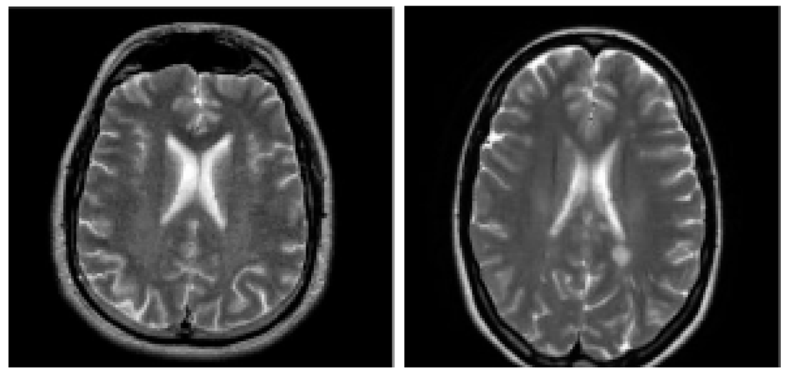
The health dataset used in the experiment was provided by Zhang [
7]. The MS images were obtained from eHealth laboratory. All cases have been experienced neurologist MS identification, and confirmed by the radiologist. Samples of healthy and MS diseased brains are showed as
Figure 1.
III. Methodology
B. Feedforward Neural Network
Artificial neural network (ANN) in machine learning is constructed by imitating the biological neural network structure of the human brain [
21]. It has nodes and internal connections between nodes [
22]. The nodes in it are programmed to behave similarly to real neurons, hence the name artificial neurons.
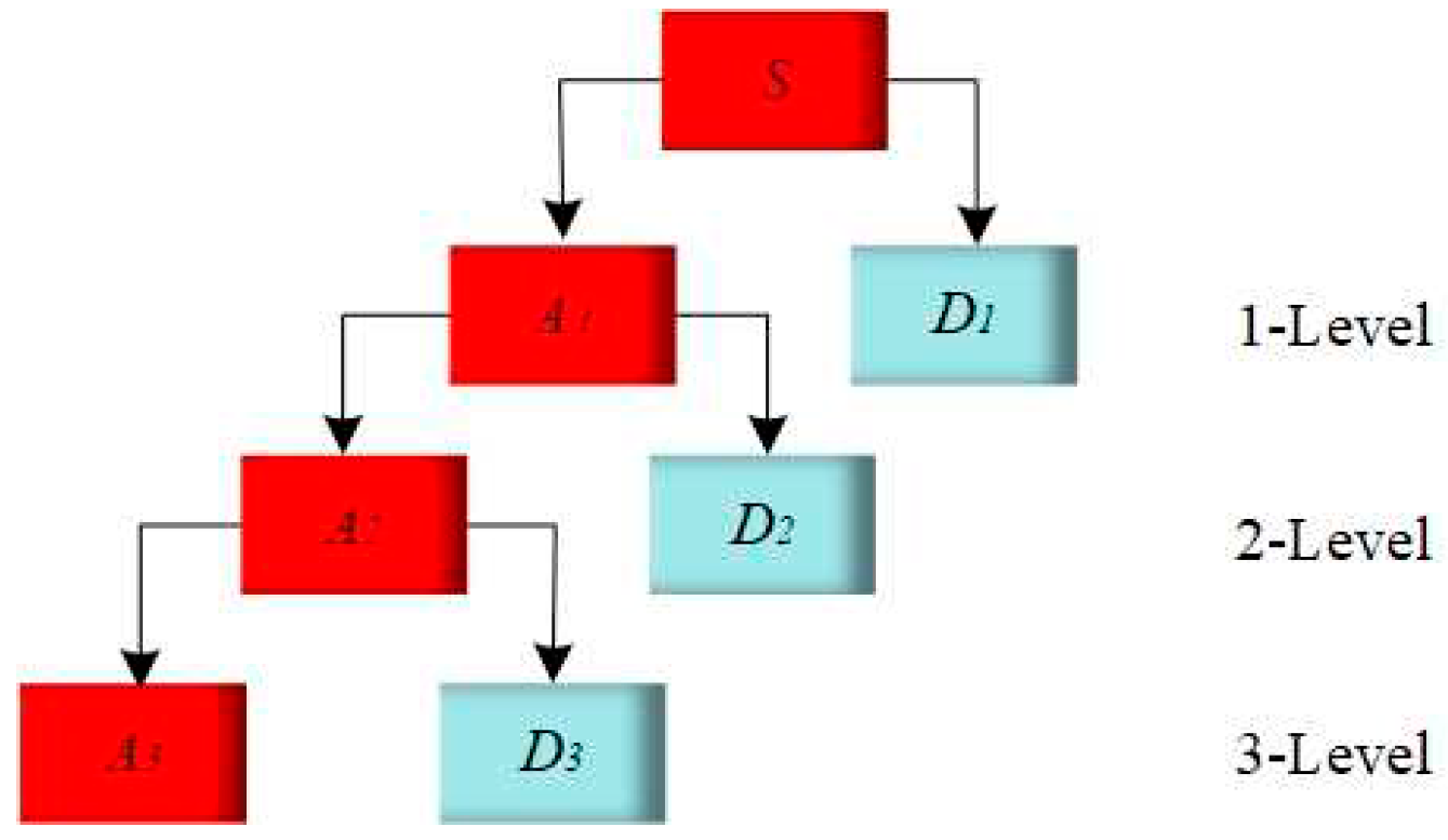
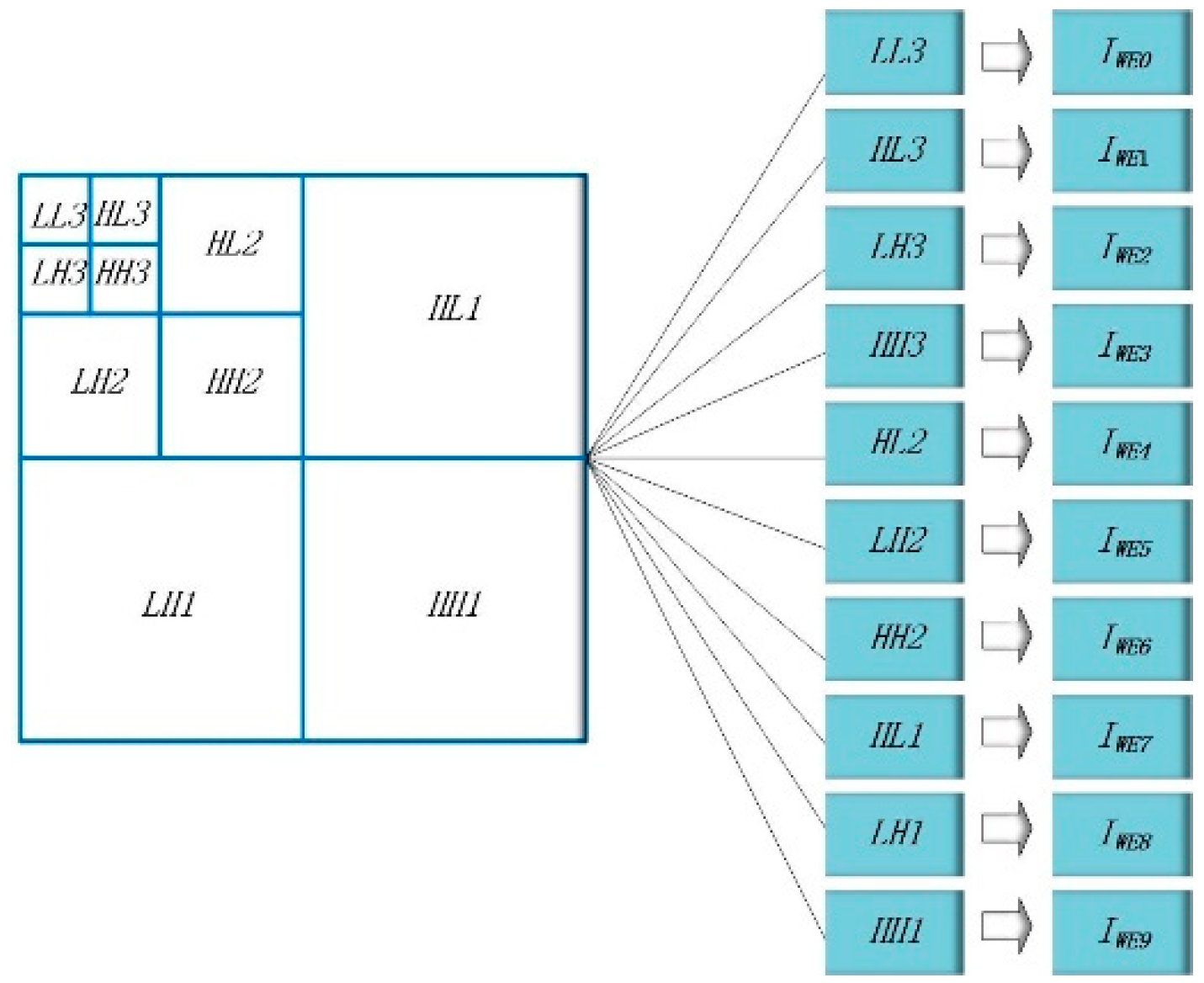
Figure 4.
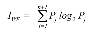
Wave entropy operation process.
Figure 4.
Wave entropy operation process.
Deep learning is to establish a set of more complex artificial neural network models on the basis of machine learning. One of the classical models is called feedforward neural network(FNN) [
23], which allows computers to build complex models through relatively simple concepts. The essence of FNN is a mathematical function, which can map a set of input data into output data. Such a complex function is composed of many simpler functions [
24].
For example, if we have three functions, they are composed to form the following function, defined as (9).
where,
f(1) represents the input layer of FNN;
f(2) represents the hidden layer of FNN;
f(3) represents the output layer of the feedforward neural network. This formula describes the simplest feedforward neural network model [
25].
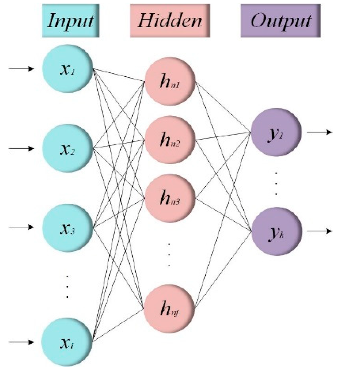
A multidimensional FNN is usually composed of input layer
xi, hidden layer
hnj and output layer
yk (where the subscript
n of
hnj is the number of hidden layers, and
j represents the number of neurons in the
n-th hidden layer) [
26]. There is no feedback in the whole network, and the signal propagates one way from the input layer to the output layer, which can be represented by a directed acyclic graph, as shown in
Figure 5.
In feedforward neural networks [
27], linear functions need to calculate the inputs of the hidden layer and the output layer. For the
j-th neuron in the
n-th hidden layer, assuming the number of inputs is
i, the corresponding linear function of the input is
f(nj)(x) as shown in (10).
The function
f(nj)(x) is a typical linear regression function [
28], where
xi is the input layer tensor, and
wij represents the connection weights between neurons in different layers. When calculating the output value of the neuron, the feedforward neural network uses a nonlinear function to calculate [
29].
In both hidden and output layers, all neurons have to employ a nonlinear activation function ∅ to calculate their output values. For the j-th neuron on the n-th hidden layer, its activation function ∅(nj) can be expressed as (11), (12).
As shown in (11) (12), the input value of any neuron in the hidden layer is the difference between
f(nj)(x) and the threshold
θnj. This difference will be used as a variable in the activation function
∅(nj) to calculate the output value [
30].
The neurons in the output layer
yk use a similar algorithm to the neurons in the hidden layer to calculate the input and output values. So, in terms of the FNN classifier, the output value
y = f(*)(x) of the output neuron represents that the input layer
x is mapped to a certain class by the FNN model [
31].
In this experiment, a FNN containing only a single hidden layer (n = l) was built. The 10 wavelet entropies extracted from the MS brain image are used as the neural network input vector , so the number of neurons in the input layer is 10 (i = 10). The MS brain detection is a binary classification problem, so the output layer contains 2 (k = 2) neurons. The number of neurons in the hidden layer is set to 40 (j = 40).
C. Self-adaptive Particle Swarm Optimisation (SaPSO)
Particle Swarm Optimization (PSO) [
32] is an optimization algorithm based on the foraging behavior of birds, which can find the optimal solution by simulating the motion and interaction of particles in the search space [
33]. It has the ability of global optimization and high efficiency and is widely used in various fields [
34]. Machine learning is an important part of modern information technology, and the application of particle swarm optimization in machine learning is more and more extensive [
35]. Particle swarm optimization can be used in neural network training, model optimization, feature selection, etc [
36].
The core of the particle swarm optimization is a continuous movement of all particles and constantly updates their locations until they converge to find the optimal location [37, 38]. The update of particle positions in particle swarm optimization follows (13).
where,
t is for time,
pi is a position vector representing the position of particle
i, and
veli is the distance and direction the particle is moving, which is calculated by (14).
where,
w is for the quality of inertia of the particle,
c1 and
c2 for acceleration constant,
r1 and
r2 to [0,1] is uniformly distributed random variables, within the scope of
Pibest for particle the best candidate for the solution of the position vector,
Pgbest is the best place for all particles [
39].
However, the particle motion path of PSO has obvious limitations [
40]. When the particle initial position path and local optimal path do not exist global optimal, the model can easily fall into local optima. In addition, the behavior of all particles moving towards the optimal solution found at the same time is a waste of computational resources [
41].
So we use SaPSO to optimize the initial weights and thresholds of the FNN to speed up the training convergence and make it reach the global optimum.
SaPSO is an optimization algorithm, which is a variant of PSO. Different from the traditional PSO, SaPSO uses an adaptive strategy to adjust the parameters of the algorithm to improve the performance and convergence speed of the algorithm.
In SaPSO, each particle has two states: the exploitation state and the exploration state. When the particle is in the utilization state, it follows the traditional PSO and moves towards the current population optimum and the individual optimum [
42]. When the particle is in the exploration state, it is far away from the current individual optimal solution and the worst solution, and searches in other directions. The speed of updating the particle position in the exploration state is calculated according to (15).
where,
Piworst represents the worst solution found by the particle
i.
The global optimal solution is finally obtained by iteratively updating the velocity and position of the particles.
D. K-fold Cross-validation
Partitioning the dataset according to data usage is an important way to avoid overfitting and improve model robustness in deep learning. However, large datasets are often difficult to obtain in many fields [
43]. Thus, partitioning the dataset leads to too few training samples, which leads to a higher probability of overfitting and a reduced robustness of the model. One of the practical solutions to such problems is cross-validation, which can improve data utilization by repeating the interrupt and partition steps [
44]. The idea of
k-fold cross-validation is as follows:
Firstly, all samples are divided into k subsets with the same size.
Each time, the current subset was used as the validation set, and all the remaining samples were used as the training set to train and evaluate the model.
Finally,

the average value (
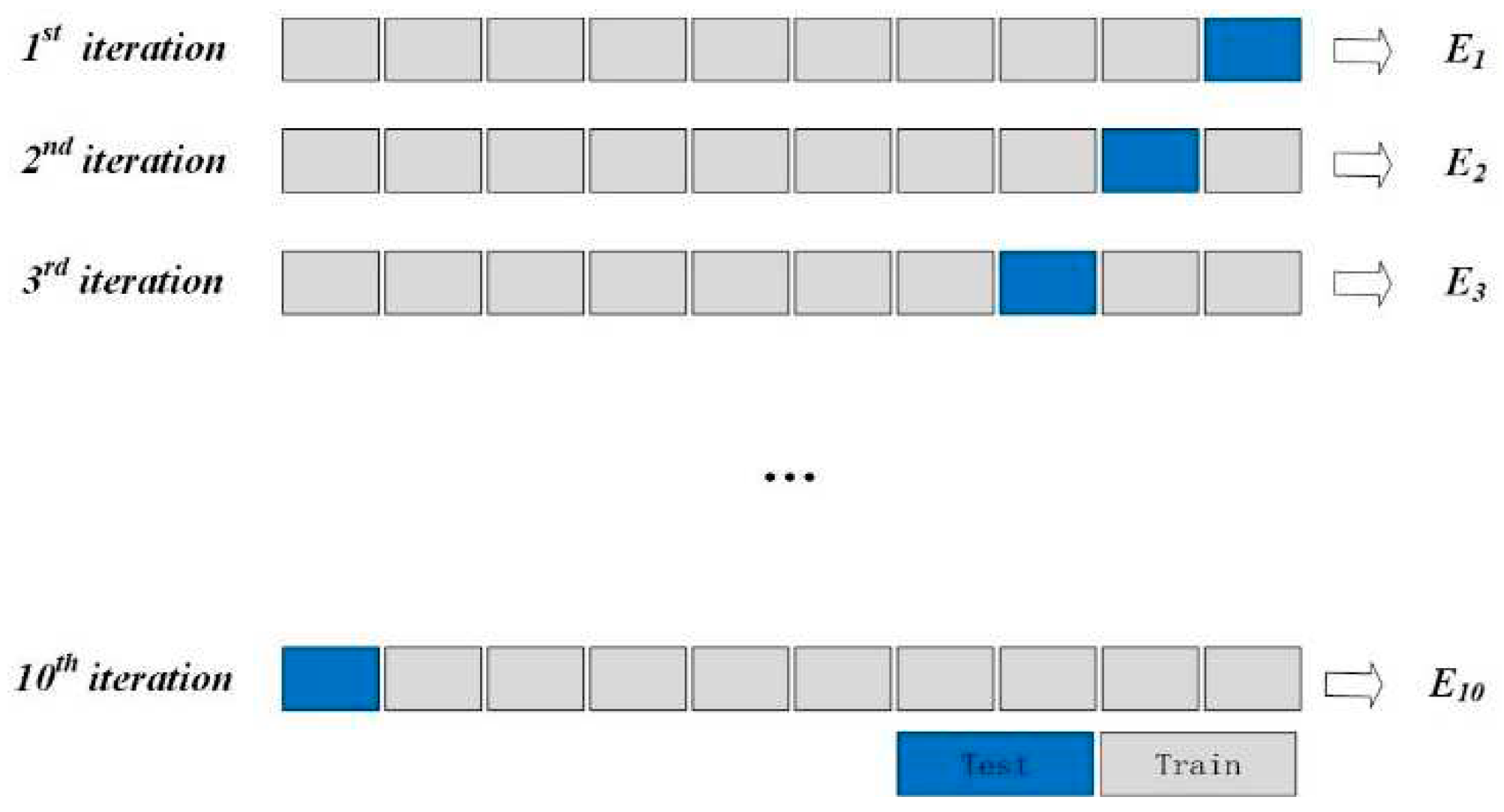
Ei,i= 0,1,2,...,9) of evaluation indicators() is taken as the final evaluation indicator. In the experiment, 10-fold cross-validation (
k = 10) is used to evaluate the performance of the detection algorithm, and the verification method is shown in
Figure 6.
IV. Experiment Results and Discussions
A. WE Results
The
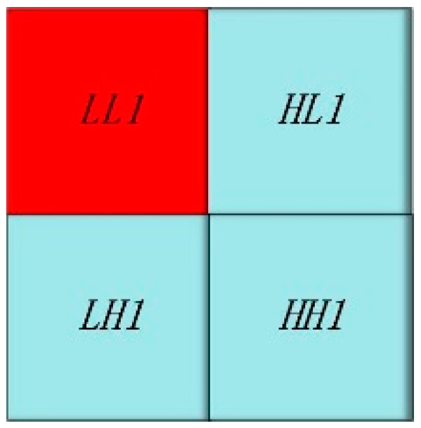
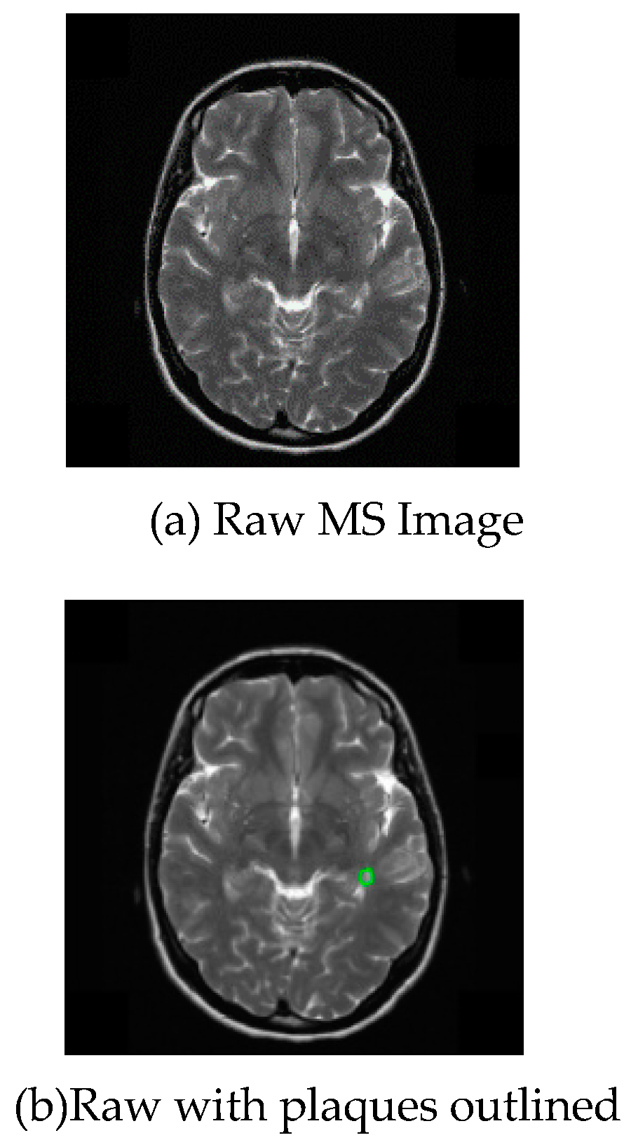
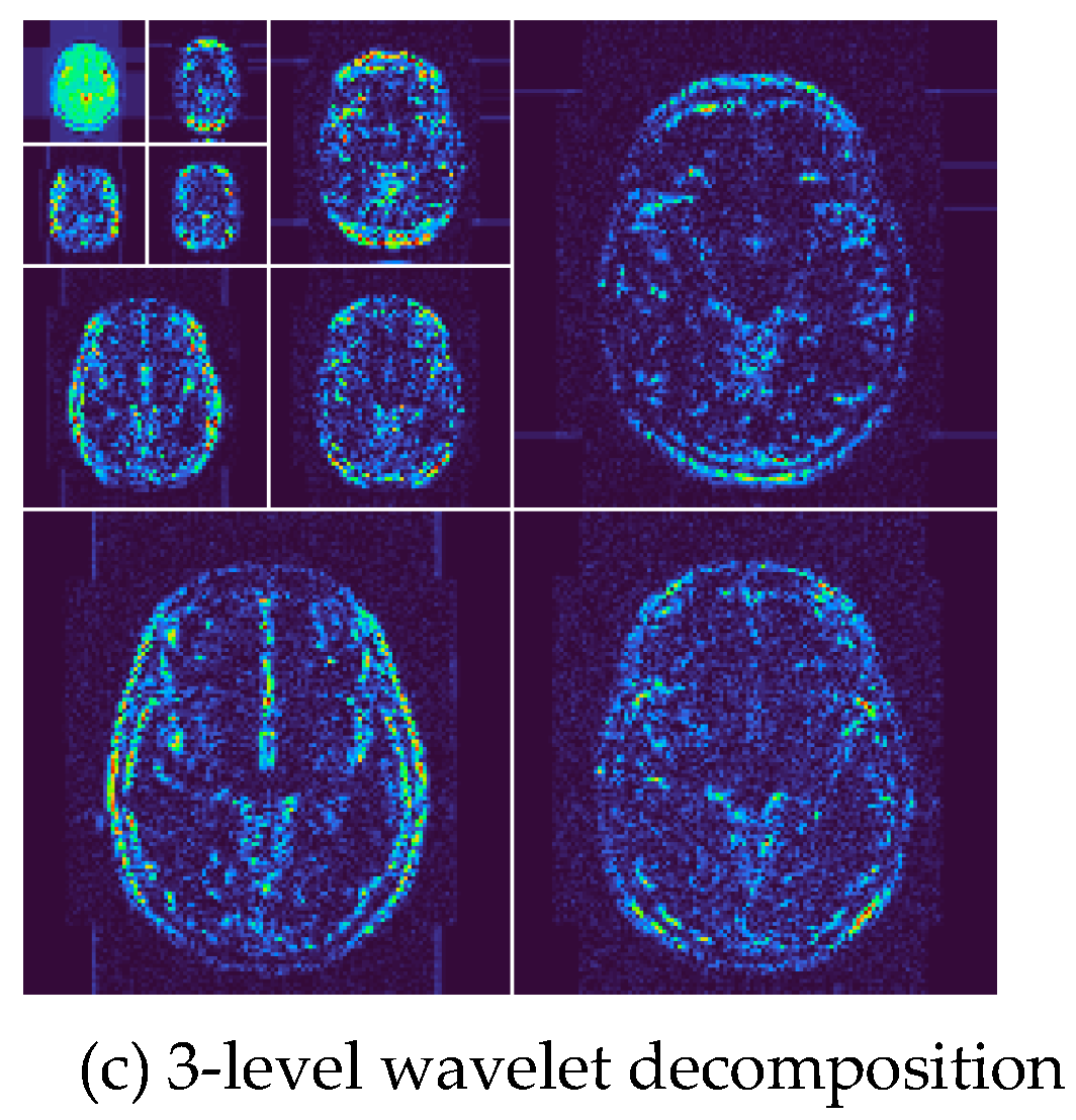
Figure 7 shows a sample of the results of the 3-level wavelet transform of this experiment, where (a) is the raw image, (b) is the raw with plaques outlined. We perform 3-level 2D-DWT on this map to decompose 10 wavelet subbands. Each level of wavelet decomposition is carried out in the approximate subband, and the other three frequency bands containing detailed information are called detailed subbands. The image (c) shows the final output of 3-level wavelet transform.
B. Statistical Results
The model is trained by SaPSO and 10-fold cross- validation is used as the data set segmentation mechanism. To evaluate the performance of our detection algorithm, we identified Specificity (SP), Sensitivity (SE), Accuracy (AC), Precision (PR), F1score, Matthews correlation coefficient (MCC) and Fowlkes-Mallows Index (FMI) as indicators.
The mean and standard deviation (MSD) is shown in
Table 1, with an average sensitivity of 92.29±1.89, specificity of 92.54±0.67, precision of 92.48±0.59, accuracy of 92.42±0.88, and F1 score of 84.85±1.74, Matthews correlation coefficient of 92.37±0.96, and Fowlkes Mallows Index of 92.38±0.96.
C. Comparison to State-of-the-art Approaches
In this paper, a detection algorithm based on WE-SaPSO is proposed to detect multiple sclerosis brain images, and this method is compared with the advanced detection algorithm proposed by four other researchers in the same field. The experimental results are shown in
Table 2.
In terms of sensitivity (SE), the result of WE-FNN-AGA is 91.91±1.24, the HMI-FNN-PSO is 91.67±1.41, DMGPS is 88.99±1.20, and WE+PSONN is 91.95±1.15. Meanwhile, the accuracy (AC) of WE-FNN-AGA and WE+PSONN reached 91.95±1.19 and 92.16±0.90, while the detection results of HMI-FNN-PSO and DMGPS were only 91.70±0.97 and 88.78±0.95, respectively.
Therefore, the experiment proves that the detection algorithm based on WE-SaPSO (ours) is more effective for the detection of multiple sclerosis brain map.
V. Conclusions
As far as possible in order to improve the efficiency of the doctor's diagnosis, reduce diagnostic time cost, this paper proposes a multiple sclerosis brain image detection based on WE-SaPSO algorithm. In the traditional FNN detection method, DWT is used to decompose the high and low frequency feature information of images, which is conducive to image recognition and classification. At the same time, the WE is used to convert the brain map into 10×1 feature vector, so as to reduce the calculation cost. Then SaPSO optimizes the feedforward neural network. SaPSO algorithm can adjust the parameters adaptively compared with the classical PSO algorithm, thus improving the convergence accuracy and speeding up the convergence speed. Therefore, this algorithm can obtain better detection results.
In future work, we will try to further expand the research from the following slowdowns:
(1) Increasing the data collection sample. There are not many data samples in the training of the model in this paper, which will have a certain impact on the test results. At the same time, the algorithm proposed in this paper can be applied to the training and testing of pneumatic disease brain map, which needs to be further implemented.
(2) In the later stage, we will consider increasing the depth of the neural network and adjusting the network structure to improve the detection accuracy, while ensuring that the computational cost is reduced and the experimental complexity is reduced.
Artificial intelligence and deep learning technologies are constantly evolving. In the future, more excellent optimization algorithms will continue to appear in medical image detection, which is of great significance to the research of medical image detection.
Funding
state key laboratory of millimeter waves (Grant No. K202218)
Acknowledgment
We would like to extend our heartfelt thanks to a host of people, without whose assistance the accomplishment of this thesis would have been impossible. This research was funded by the open project of State Key Laboratory of Millimeter Waves (Grant No. K202218).
References
- J. Han and S.-M. Hou, "Multiple Sclerosis Detection via Wavelet Entropy and Feedforward Neural Network Trained by Adaptive Genetic Algorithm," in Advances in Computational Intelligence, Cham, 2019, pp. 87-97.
- N. Aslam, I. U. Khan, A. Bashamakh, F. A. Alghool, M. Aboulnour, N. M. Alsuwayan, et al., "Multiple Sclerosis Diagnosis Using Machine Learning and Deep Learning: Challenges and Opportunities," vol. 22, p. 7856, 2022. [CrossRef]
- M. Kaya, S. Karakuş, and S. A. Tuncer, "Detection of ataxia with hybrid convolutional neural network using static plantar pressure distribution model in patients with multiple sclerosis," Computer Methods and Programs in Biomedicine, vol. 214, p. 106525, 2022. [CrossRef]
- J. Han and S.-M. Hou, "A Multiple Sclerosis Recognition via Hu Moment Invariant and Artificial Neural Network Trained by Particle Swarm Optimization," in Multimedia Technology and Enhanced Learning, Cham, 2020, pp. 254-264.
- Y. Zhao and T. Chitnis, "Dirichlet Mixture of Gaussian Processes with Split-kernel: An Application to Predicting Disease Course in Multiple Sclerosis Patients," in 2022 International Joint Conference on Neural Networks (IJCNN), 2022, pp. 1-8.
- D. Lima, "Multiple Sclerosis Recognition via Wavelet Entropy and PSO-Based Neural Network," in Preprints, ed: Preprints, 2023.
- Y.-D. Zhang, "Multiple sclerosis identification by convolutional neural network with dropout and parametric ReLU," Journal of Computational Science, vol. 28, pp. 1-10, 2018. [CrossRef]
- S. A. Agnes, A. A. Solomon, and K. Karthick, "Wavelet U-Net plus plus for accurate lung nodule segmentation in CT scans: Improving early detection and diagnosis of lung cancer," Biomedical Signal Processing and Control, vol. 87, Article ID: 105509, 2024.
- Y.-x. Li, S.-b. Jiao, and X. Gao, "A novel signal feature extraction technology based on empirical wavelet transform and reverse dispersion entropy," Defence Technology, vol. 17, pp. 1625-1635, 2021. [CrossRef]
- F. A. Alturki, K. AlSharabi, A. M. Abdurraqeeb, and M. Aljalal, "EEG Signal Analysis for Diagnosing Neurological Disorders Using Discrete Wavelet Transform and Intelligent Techniques," vol. 20, p. 2505, 2020. [CrossRef]
- S. Lu, Z. Lu, J. Yang, M. Yang, and S. Wang, "A pathological brain detection system based on kernel based ELM %J Multimedia tools and applications %J," vol. 77, pp. 3715-3728, 2018.
- C. H. Liu and A. H. Wang, "An image zooming method based on the coupling threshold in the wavelet packet transform domain," Measurement Science and Technology, vol. 35, Article ID: 015408, 2024. [CrossRef]
- V. B. Awati, A. Goravar, and M. N. Kumar, "Spectral and Haar wavelet collocation method for the solution of heat generation and viscous dissipation in micro-polar nanofluid for MHD stagnation point flow," Mathematics and Computers in Simulation, vol. 215, pp. 158-183, 2024. [CrossRef]
- Y. M. Krishna and P. V. Kumar, "Efficient automated method to extract EOG artifact by combining Circular SSA with wavelet and unsupervised clustering from single channel EEG," Biomedical Signal Processing and Control, vol. 87, Article ID: 105455, 2024.
- V. K. Sharma, S. Singh, R. Pandey, and G. P. Singh, "Estimation of approximation error of a function having its derivatives belonging to Lipschitz class of order- α by extended Legendre wavelet (ELW) method and its applications," Filomat, vol. 38, pp. 67-98, 2024.
- S. Ullah, R. D. Luo, T. S. Adebayo, and D. Balsalobre-Lorente, "Green perspectives of finance, technology innovations, and energy consumption in restraining carbon emissions in China: Fresh insights from Wavelet approach," Energy Sources Part B-Economics Planning and Policy, vol. 18, Article ID: 2255584, 2023. [CrossRef]
- N. Burud and J. C. Kishen, "Damage detection using wavelet entropy of acoustic emission waveforms in concrete under flexure," vol. 20, pp. 2461-2475, 2021. [CrossRef]
- S.-H. Wang, "Unilateral sensorineural hearing loss identification based on double-density dual-tree complex wavelet transform and multinomial logistic regression," Integrated Computer-Aided Engineering, vol. 26, pp. 411-426, 2019. [CrossRef]
- Y. Zhang, "Feature Extraction of Brain MRI by Stationary Wavelet Transform and its Applications," Journal of Biological Systems, vol. 18, pp. 115-132, 2010. [CrossRef]
- J. Zhuang, Q. Peng, F. Wu, and B. Guo, "Multi-component attention-based convolution network for color difference recognition with wavelet entropy strategy," Advanced Engineering Informatics, vol. 52, p. 101603, 2022. [CrossRef]
- H. J. Wu, R. S. Lei, Y. B. Peng, and L. Gao, "AAGNet: A graph neural network towards multi-task machining feature recognition," Robotics and Computer-Integrated Manufacturing, vol. 86, Article ID: 102661, 2024. [CrossRef]
- Y. Zhang, "Smart detection on abnormal breasts in digital mammography based on contrast-limited adaptive histogram equalization and chaotic adaptive real-coded biogeography-based optimization," Simulation, vol. 92, pp. 873-885, 2016. [CrossRef]
- T. Fang, C. Zheng, and D. Wang, "Forecasting the crude oil prices with an EMD-ISBM-FNN model," Energy, vol. 263, p. 125407, 2023. [CrossRef]
- U. Lee and I. Lee, "Efficient sampling-based inverse reliability analysis combining Monte Carlo simulation (MCS) and feedforward neural network (FNN)," Structural and Multidisciplinary Optimization, vol. 65, p. 8, 2021. [CrossRef]
- W. H. Guo and Y. J. Wang, "Convolutional gated recurrent unit-driven multidimensional dynamic graph neural network for subject-independent emotion recognition," Expert Systems with Applications, vol. 238, Article ID: 121889, 2024. [CrossRef]
- Z. L. Liu, P. Zhao, J. Cao, J. L. Zhang, and Z. H. Chen, "A constrained multi-objective evolutionary algorithm with Pareto estimation via neural network," Expert Systems with Applications, vol. 237, Article ID: 121718, 2024. [CrossRef]
- S.-H. Wang, "Diagnosis of COVID-19 by Wavelet Renyi Entropy and Three-Segment Biogeography-Based Optimization," International Journal of Computational Intelligence Systems, vol. 13, pp. 1332-1344, 2020. [CrossRef]
- G. Zhang, X. Wang, L. Li, and X. Zhao, "Tire-Road Friction Estimation for Four-Wheel Independent Steering and Driving EVs Using Improved CKF and FNN," IEEE Transactions on Transportation Electrification, pp. 1-1, 2023. [CrossRef]
- Y. D. Zhang and S. Satapathy, "A seven-layer convolutional neural network for chest CT-based COVID-19 diagnosis using stochastic pooling," IEEE Sensors Journal, vol. 22, pp. 17573 - 17582, 2022. [CrossRef]
- M. Taimoor, X. Lu, W. Shabbir, and C. Sheng, "Neural network observer based on fuzzy auxiliary sliding-mode-control for nonlinear systems," Expert Systems with Applications, vol. 237, p. 121492, 2024. [CrossRef]
- X. Yao, Z. Zhu, C. Kang, S. H. Wang, J. M. Gorriz, and Y. D. Zhang, "AdaD-FNN for Chest CT-Based COVID-19 Diagnosis," IEEE Transactions on Emerging Topics in Computational Intelligence, vol. 7, pp. 5-14, 2023.
- M. Bey, P. Kuila, B. B. Naik, and S. Ghosh, "Quantum-inspired particle swarm optimization for efficient IoT service placement in edge computing systems," Expert Systems with Applications, vol. 236, Article ID: 121270, 2024. [CrossRef]
- S. K. Rawat, M. Yaseen, M. Pant, C. S. Ujarari, D. K. Joshi, S. Chaube, et al., "Designing soft computing algorithms to study heat transfer simulation of ternary hybrid nanofluid flow between parallel plates in a parabolic trough solar collector: Case of artificial neural network and particle swarm optimization," International Communications in Heat and Mass Transfer, vol. 148, Article ID: 107011, 2023. [CrossRef]
- W. C. Sugianto and B. S. Kim, "Particle swarm optimization for integrated scheduling problem with batch additive manufacturing and batch direct-shipping delivery," Computers & Operations Research, vol. 161, Article ID: 106430, 2024. [CrossRef]
- X. T. Li, W. Fang, and S. W. Zhu, "An improved binary quantum-behaved particle swarm optimization algorithm for knapsack problems," Information Sciences, vol. 648, Article ID: 119529, 2023. [CrossRef]
- A. Soltanisarvestani, A. A. Safavi, and M. A. Rahimi, "The Detection of Unaccounted for Gas in Residential Natural Gas Customers Using Particle Swarm Optimization-based Neural Networks," Energy Sources Part B-Economics Planning and Policy, vol. 18, Article ID: 2154412, 2023. [CrossRef]
- A. Al-Ali, U. Qidwai, and S. Kamran, "Predicting infarction growth rate II using ANFIS-based binary particle swarm optimization technique in ischemic stroke," Methodsx, vol. 11, Article ID: 102375, 2023. [CrossRef]
- Y. F. Lu, B. D. Li, S. C. Liu, and A. M. Zhou, "A Population Cooperation based Particle Swarm Optimization algorithm for large-scale multi-objective optimization," Swarm and Evolutionary Computation, vol. 83, Article ID: 101377, 2023. [CrossRef]
- T. Fei, A. A. Zhang, Y. Jie, and C. Lin, "Inversion analysis of rock mass permeability coefficient of dam engineering based on particle swarm optimization and support vector machine: A case study," Measurement, vol. 221, Article ID: 113580, 2023. [CrossRef]
- I. Choulli, M. Elyaqouti, E. Arjdal, D. Ben Hmamou, D. Saadaoui, S. Lidaighbi, et al., "Hybrid optimization based on the analytical approach and the particle swarm optimization algorithm (Ana-PSO) for the extraction of single and double diode models parameters," Energy, vol. 283, Article ID: 129043, 2023. [CrossRef]
- X. Li, S. Xu, M. Yu, K. Wang, Y. Tao, Y. Zhou, et al., "Risk factors for severity and mortality in adult COVID-19 inpatients in Wuhan," J Allergy Clin Immunol, vol. 146, pp. 110-118, 2020. [CrossRef]
- W. Wang, S.-H. Wang, J. M. Górriz, and Y.-D. Zhang, "Covid-19 Detection by Wavelet Entropy and Self-adaptive PSO," in Artificial Intelligence in Neuroscience: Affective Analysis and Health Applications, Cham, 2022, pp. 125-135.
- T. T. Wong and P. Y. Yeh, "Reliable Accuracy Estimates from k-Fold Cross Validation," IEEE Transactions on Knowledge and Data Engineering, vol. 32, pp. 1586-1594, 2020. [CrossRef]
- X. Zhang and C.-A. Liu, "Model averaging prediction by K-fold cross-validation," Journal of Econometrics, vol. 235, pp. 280-301, 2023. [CrossRef]
|
Disclaimer/Publisher’s Note: The statements, opinions and data contained in all publications are solely those of the individual author(s) and contributor(s) and not of MDPI and/or the editor(s). MDPI and/or the editor(s) disclaim responsibility for any injury to people or property resulting from any ideas, methods, instructions or products referred to in the content. |
© 2023 by the authors. Licensee MDPI, Basel, Switzerland. This article is an open access article distributed under the terms and conditions of the Creative Commons Attribution (CC BY) license (http://creativecommons.org/licenses/by/4.0/).
 ; So continuous wavelet transform(CWT) is defined as (1).

 is called wavelet.
 then
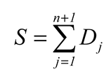
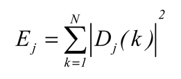
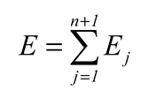
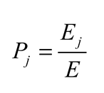
then

 .
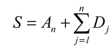
.


 the average value (Ei,i= 0,1,2,...,9) of evaluation indicators() is taken as the final evaluation indicator. In the experiment, 10-fold cross-validation (k = 10) is used to evaluate the performance of the detection algorithm, and the verification method is shown in Figure 6.