1. Introduction
Olive, Olea europaea, is an essential evergreen subtropical fruit. Its fruits are utilized for both table olives and olive oil. Certain varieties are specifically cultivated for oil production, while others, renowned for their larger fruit sizes, are preferred for canning products. Moreover, the production of dual-purpose olive varieties is growing (Fabbri et al., 2023). In Iran, the `Roghani` cultivar stands out as a vital local dual-purpose olive variety, known for its adaptability to diverse environmental conditions and ability to withstand winter cold (Rezaei & Rohani, 2023). The type of canned olives and the quality of olive oil depend on various factors, including the variety, cultivation conditions, and fruit ripening stage (Boskou, 2006; Lazzez et al., 2008; mohamed Diab et al., 2020). Olive fruits can be harvested at different stages, ranging from immature green to fully mature black, and even during over-ripened stages. The ripening stage of the fruit profoundly affects the oil content, chemical composition, sensory characteristics of olive oil, and industrial yield (Jiménez et al., 2013; Pereira, 2013). Fruit homogeneity at the same ripening stage is crucial for canned olives, and the quality of olive oil directly depends on the fruit's ripening stage.
The timing of olive harvesting is typically determined by evaluating the maturity index (MI) of each olive cultivar (Famiani et al., 2002; Guzmán et al., 2015; Lazzez et al., 2008). This evaluation of MI is based on changes in both the skin and flesh color of mature fruit (Bellincontro et al., 2012). Decisions about when to harvest fruit from an orchard are made by conducting MI assessments on fruit samples collected from different trees. However, it is common to come across olives with varying degrees of ripeness during processing, as mechanical harvesters that use trunk shakers can harvest one hectare of an intensive olive grove (consisting of 300-400 trees) within a timeframe of 2 to 5 days (Bellincontro et al., 2012). Due to factors such as the location of the fruit on outer or inner branches and exposure to sunlight, even a single tree may have olives in different stages of maturity, and there may be variations between each tree due to differences in horticultural practices and management. Moreover, some orchards may cultivate multiple olive varieties, each with distinct ripening stages during harvest, while others with a single cultivar may also have variations in fruit ripeness. In olive processing facilities, it is possible for different growers to bring olives with varying degrees of ripeness that must be categorized before processing.
Given the importance of olive ripening in the production of various postharvest products, such as pickles, oil, and canned olives, it is essential to separate and sort olive fruits before processing. However, manually sorting olives through human visual inspection is a challenging and inefficient task. To address this challenge, integrating a computer vision system into olive processing units as part of the automatic separation machinery offers a potential solution. The system consists of an image-capturing unit, which relies on a robust image processing model to ensure rapid and accurate results for mechanical separation (Violino et al., 2022).
Numerous researchers have investigated various methods for assessing olive fruit maturity, with a focus on Near Infrared Spectroscopy (NIRS) (e.g., Bellincontro et al., 2012; Gracia & León, 2011; Salguero-Chaparro et al., 2012). These studies aimed to predict diverse quality parameters and characterize table olive traits utilizing NIRS technology. Besides NIRS, Convolutional Neural Networks (CNNs), a subset of deep learning, have emerged as powerful tools for image processing tasks, allowing for the extraction of high-level features independent of imaging conditions and structures (Wu et al., 2020), making them a valuable tool for agricultural applications.
The use of cutting-edge technologies, such as deep learning, offers a more promising solution to address this challenge, garnering the attention of scientists across multiple agricultural domains (Kamilaris & Prenafeta-Boldú, 2018; Khosravi et al., 2021; Saedi & Khosravi, 2020). Noteworthy applications of CNNs include olive classification, as demonstrated by Riquelme et al., (2008), who employed discriminant analysis to classify olives based on external damage in images, achieving validation accuracies ranging from 38% to 100%. Guzmán et al., (2015) leveraged algorithms based on color and edge detection for image segmentation, resulting in an impressive 95% accuracy in predicting olive maturity. Ponce et al., (2019) utilized the Inception-ResNetV2 model to classify seven olive fruit varieties, achieving a remarkable maximum accuracy of 95.91%. Aguilera Puerto et al., (2019) developed an online system for olive fruit classification in the olive oil production process, employing Artificial Neural Networks (ANN) and Support Vector Machines (SVM) to attain high accuracies of 98.4% and 98.8%, respectively. Aquino et al., (2020) created an artificial vision algorithm capable of classifying images taken in the field to identify olives directly from trees, enabling accurate yield predictions. Studies such as Khosravi et al., (2021), have also utilized RGB image acquisition and CNNs for the early estimation of olive fruit ripening stages on-branch, which has direct implications for orchard production quality and quantity. Furferi et al., (2010) proposed an ANN-based method for automatic maturity index evaluation, considering four classes based on olive skin and pulp color, while ignoring the presence of defects. In contrast, Puerto et al., (2015) implemented a static computer vision system for olive classification, employing a shallow learning approach using an ANN with a single hidden layer. In a recent study by Figorilli et al., (2022), olive fruits were classified based on the state of external veraison and the presence of visible defects using AI algorithms with RGB imaging.
The field of machine learning has seen significant advancements in recent years, particularly in agriculture. According to Benos et al., (2021), there was a remarkable 745% increase in articles related to machine learning in agriculture between 2018 and 2020, indicating the growing use of machine learning algorithms for crop and animal analysis based on input data from satellites and drones. This surge in interest is attributed to the development of novel models that exhibit high performance and optimized detection times. For instance, Fan et al., (2022), successfully utilized a YOLOV4 network to detect defects in apple fruits using near-infrared (NIR) images, achieving an average detection accuracy of 93.9% and processing five fruits per second.
In the realm of fruit recognition, the Xception deep learning model has been gainfully employed (Salim et al., 2023). Built upon the Inception architecture, Xception is a powerful neural network that excels in image classification tasks owing to its efficiency and accuracy (Chollet, 2017). By taking the concept of separable convolutions to an extreme level, Xception becomes a highly efficient and powerful network, demonstrating the potential of CNNs for image processing tasks.
This study aims to leverage the Xception deep learning model for the automated sorting of olives based on color images, given the critical role of olive fruit sorting in producing diverse end products (e.g., pickles, oil, canned goods). Our ultimate goal is to create a highly accurate and robust computer vision system capable of categorizing 'Roghani' olives into five distinct ripening stages. We will evaluate the system's performance using test dataset accuracy, classification performance metrics (such as classification reports and confusion matrices), and its capacity to generalize well across varied datasets.
The significance of our research lies in its potential to offer olive processing facilities efficient and reliable tools for automating the sorting process, thus distinguishing between olives of differing ripeness levels. This, in turn, may enhance the quality of various post-harvest products and differentiate olive oil qualities, ultimately benefiting the olive industry as a whole. By providing a more accurate method for sorting olives according to their maturity, we can improve the overall quality of downstream products such as pickles, oil, and canned goods. Moreover, our proposed approach could potentially reduce waste and increase efficiency within the olive processing industry.
2. Material and methods
2.1. Data preparation
To develop an image-based CNN model for classifying olive fruits based on their ripening stages, we considered an Iranian olive cultivar named Roghani at five distinct ripening stages. A total of 761 images of different classes were captured in an unstructured laboratory setting using a smartphone camera. The captured images had an initial resolution of 3000 × 4000 pixels.
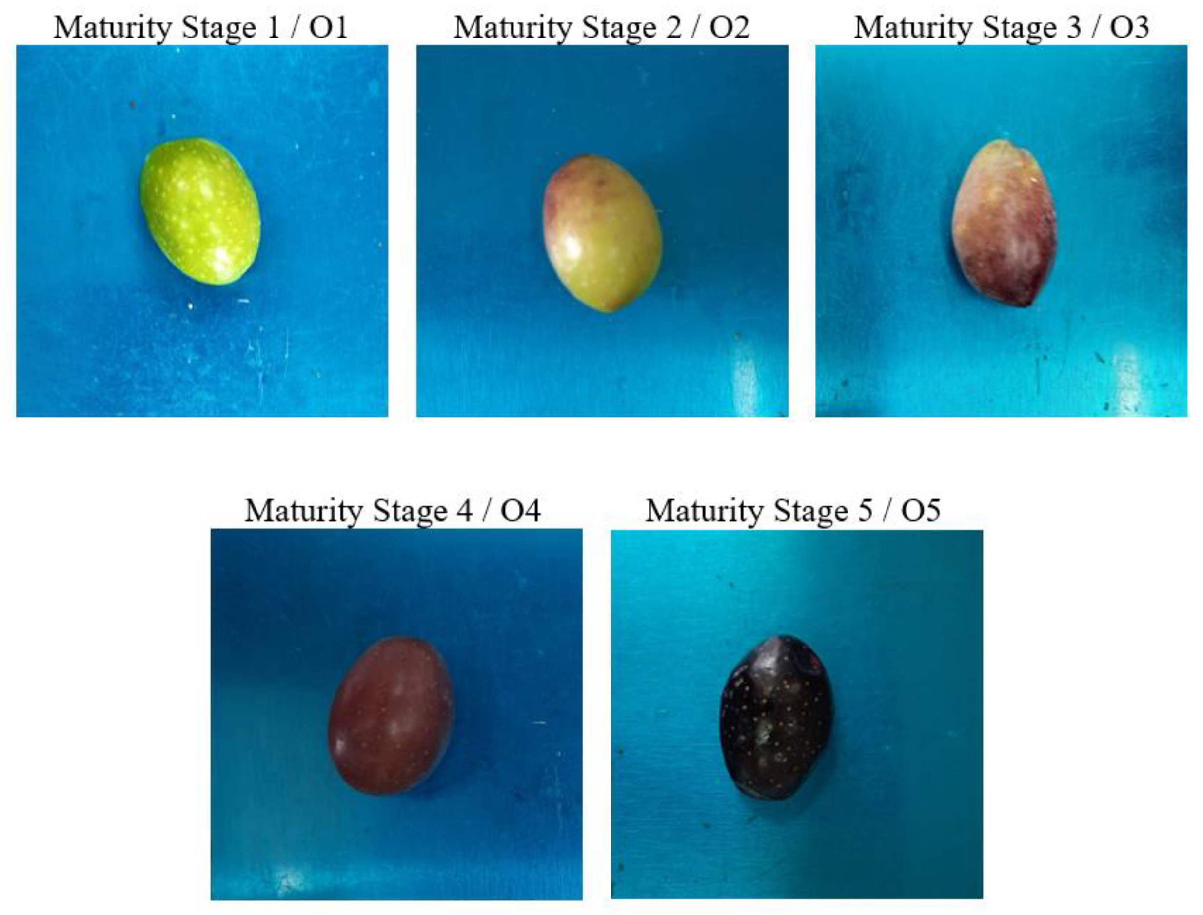
Figure 1 depicts the five ripening stages of the olive fruits and their corresponding average mass. The color attributes of the samples served as the basis for discriminating between ripening stages. Specifically, Stage 1 refers to samples with green colors, Stage 2 is characterized by olives with 10-30% browning, while Stages 3, 4, and 5 represent approximately 50, 90, and 100% browning (fully black), respectively. The number of images taken at each ripening stage, and the average mass of samples at each class, are presented in
Table 1.
The available image data was divided into three parts: training, validation, and testing sets. We allocated 60% of the data for training, 15% for validation, and 20% for testing. The training process involved passing the input data through several layers, obtaining the output, and comparing it with the desired output. The difference between the two, which served as the error, was then calculated. Using this error, the network parameters were adjusted and fed the data back into the network to compute new results and errors. This process was repeated multiple times, adjusting the parameters after each iteration to minimize the error. There are various formulas and functions to calculate the network error. Once the error was computed, the parameters were updated to move closer to minimizing it, that is, optimizing the weights to achieve the lowest possible error.
Preprocessing the input images is crucial to enhance the model's accuracy, prevent overfitting, and boost its generalization capability. First, we resized all images to two different sizes: 224 × 224 and 299 × 299. Next, we normalized the images by dividing their size by the maximum size of the captured images. Subsequently, we applied data augmentation techniques, including random translation, random flip, random contrast, and random rotation, to artificially increase the number of images used in model development. The data augmentation parameters are presented in
Table 2.
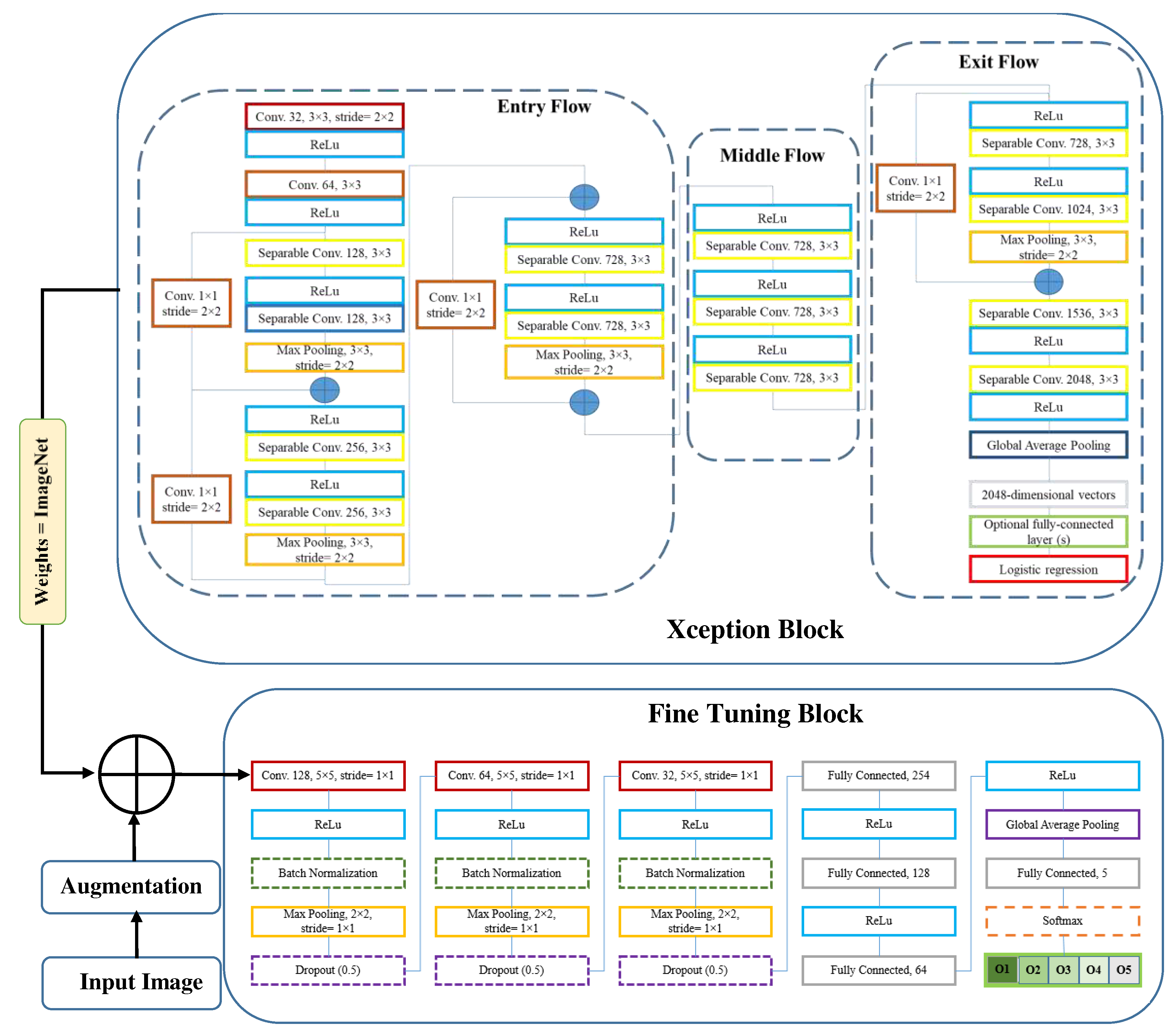
To develop the deep neural network model, we utilized the transfer learning technique. Initially, we invoked the Xception model and loaded its weights from the ImageNet dataset. Subsequently, we embarked on a fine-tuning process by adding additional layers to the base model. Diverse structures for the fine-tuning layers were experimented with, varying their type, position, and arguments to identify the optimal configuration. We explored several layer types and arrangements, with the most commonly used being 2D convolution, Global Average Pooling, Dropout, Batch Normalization, and others. The comprehensive architecture of the resulting model is illustrated in
Figure 2.
2.2. Xception Architecture
In this study, we employed the Xception deep learning architecture, a novel deep convolutional neural network model introduced by Google, Inc. (Chollet, 2017). Xception features Depth Wise Separable Convolutions (DSC) to enhance performance and efficiency. Unlike traditional convolution, DSC divides the computation into two stages: depth wise convolution applies a single convolutional filter per input channel, followed by point wise convolution to create a linear combination of the depth wise convolution outputs.
Xception is a variant of the Inception architecture where Inception modules act as an intermediate step between regular convolution and DSC. With the same number of parameters, Xception surpasses Inception V3 on the ImageNet dataset due to its more efficient use of model parameters. The Xception architecture consists of 36 convolutional layers forming the feature extraction base of the network. In image classification tasks, the convolutional base is succeeded by a logistic regression layer. The 36 convolutional layers are organized into 14 modules, all with linear residual connections around them, excluding the first and last modules. In summary, the Xception architecture is a linear stack of depth wise separable convolution layers with residual connections (Chollet, 2017).
2.2. Fine-tuning
We first pre-trained the base model (Xception) using ImageNet weights. Next, the trainable attribute of all layers in the base model were frozen, ensuring that their weights remained fixed during training. This allowed us to use the pre-trained model as a starting point for further training on a new dataset. We then unfroze the last 20 layers in the Middle Flow and Exit Flow, making them trainable. By doing so, the pre-trained layers were prevented from overfitting on the new dataset while allowing the newly added layers to adapt to the new data. Finally, we added three blocks on top of the pre-trained base model, each containing Convolution, Batch Normalization, Max Pooling, and Dropout layers, followed by Fully Connected and Global Average Pooling layers (
Figure 2).
Table 3 provides detailed information about the various layers used, their output shapes, and the total number of parameters. The table covers both input image sizes studied (224 × 224 and 299 × 299). The developed model has approximately 27 million parameters for both image sizes, with only about 0.5% being non-trainable. Notably, Max Pooling, Dropout, and Global Average Pooling layers do not contribute to the total number of trainable parameters since they lack trainable parameters. As seen in
Table 3, the number of parameters remains constant across both input image sizes.
2.3. Network training
To optimize the performance of the deep learning model for classifying olive fruits based on their ripening stages, several aspects required careful consideration. First, we needed to select the most appropriate optimizer among popular choices such as RMSprop, SGD, Adam, and Nadam. Accuracy was chosen as the evaluation metric to assess the model's performance. Additionally, we employed the categorical cross-entropy function as the loss function.
Training the model involved a series of experiments to identify the best combination of hyper parameters and architectural components. Initially, we trained the model without fine-tuning, using a batch size of 8 and 20 epochs. Subsequently, we fine-tuned the model by adding additional layers and training it with a batch size of 32 and 80 epochs (with an optional extension to 100 epochs for Model 1). Throughout the training process, we monitored the loss and accuracy trends for both the train and validation datasets at each epoch. This allowed us to analyze the models' performance and make informed decisions regarding their suitability for our task. Four promising candidates emerged from our experiments, each distinguished by its unique combination of image size and optimizer. They were:
- Model 1: Best performer with 224 × 224 image size and Nadam optimizer
- Model 2: Best performer with 224 × 224 image size and SGD optimizer
- Model 3: Best performer with 299 × 299 image size and RMSprop optimizer
- Model 4: Best performer with 299 × 299 image size and SGD optimizer
When evaluating these models, we considered multiple factors, such as accuracy, loss, and resistance to overfitting. Accuracy measures the proportion of correctly predicted instances, while loss represents the average error per instance. A lower loss value generally indicates better model performance. However, a model with high accuracy but excessively high loss may still encounter challenges in unseen data, signaling potential overfitting issues. Therefore, we assessed the risk of overfitting when comparing the four candidates.
The training, development, and testing procedures were executed using Python and the Google Colab environment (K80 GPU and 12GB RAM) with Keras, TensorFlow backend (version 2.13.0), OpenCV, and other relevant libraries.
3. Results and Discussion
This section presents the methodological approach taken to develop and evaluate deep learning models for classifying olive fruits according to their ripeness levels. Our next step will be analyzing the results and discussing the implications of our findings.
3.1. Training progress
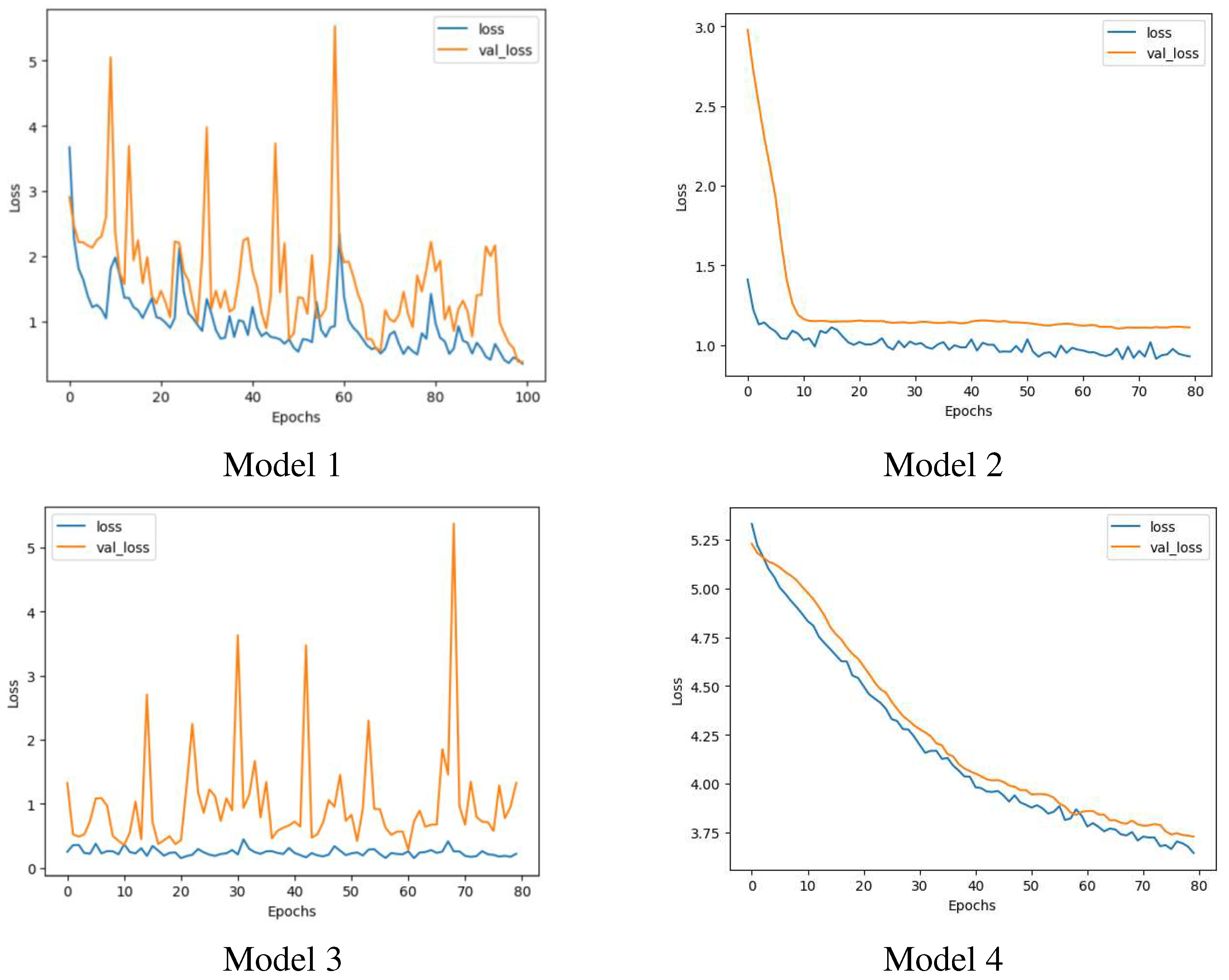
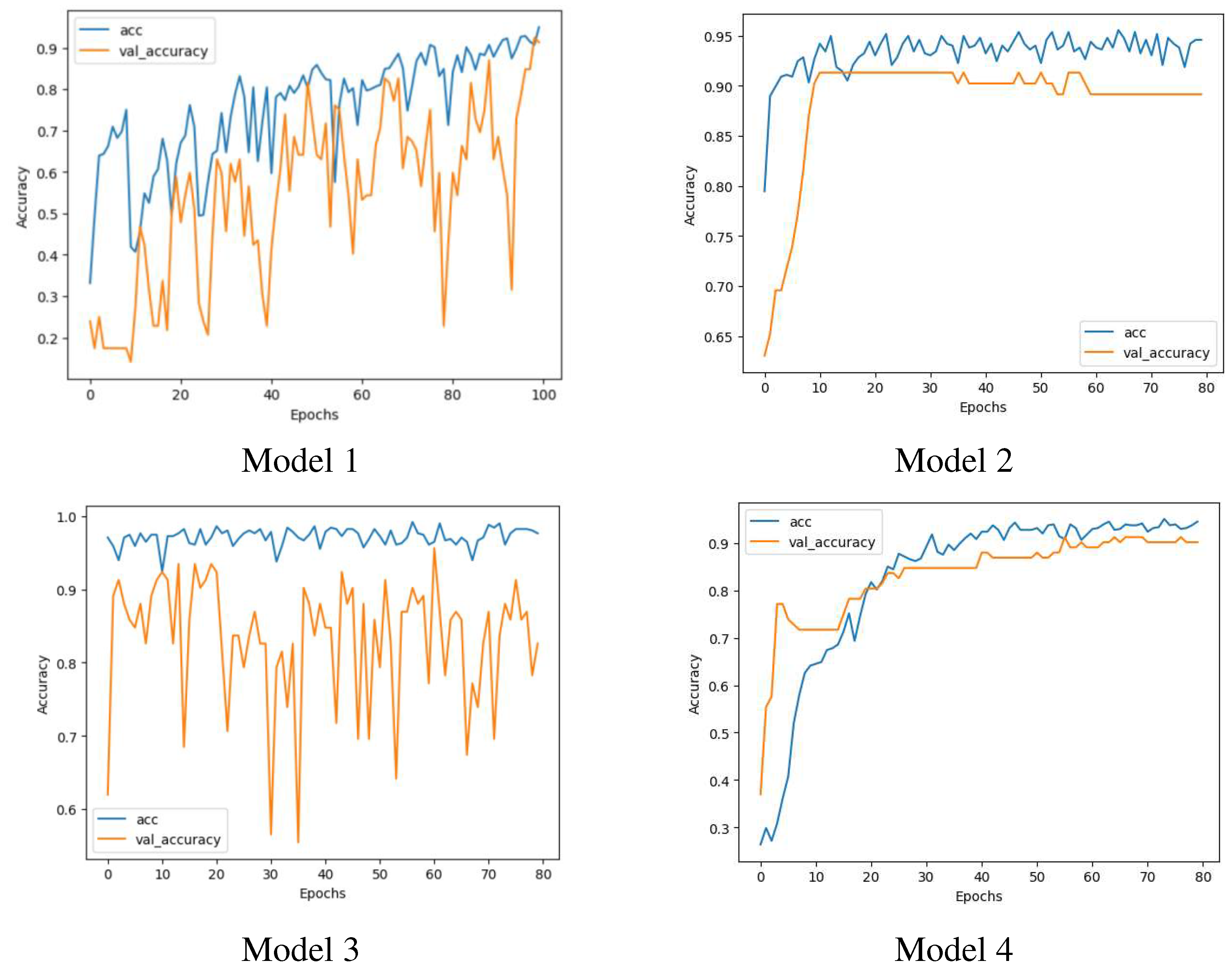
The trend of losses and accuracies against the number of epochs for both the train and validation datasets and for the four candidate models are illustrated in Figure 3 and
Figure 4. For each candidate model, the minimum losses and maximum accuracies for train and validation data and the corresponding epochs are mentioned in
Table 4.
According to
Figure 4 and
Figure 5, Models 1 and 3 exhibit substantial fluctuations in validation losses and validation accuracies, whereas Models 2 and 4 display a consistent downward trend in losses and a steady increase in accuracies, with only minor variations. These patterns suggest that Models 1 and 3 are susceptible to overfitting, whereas Models 2 and 4 are more resistant to it, making them more generalized and reliable in handling new, unseen data.
3.2. Comparison of the candidate models
Four candidate models perform differently on unseen (test) data. The result of loss and accuracy values on test data are provided in
Table 5.
According to
Table 5, both image sizes can provide low losses and high accuracies. Model 1 has the lowest test loss (0.3938) and highest test accuracy (0.9346), indicating good performance on the test set. However, test loss and test accuracy should not be the only factors considered when evaluating a CNN model, as another important factor is the risk of overfitting, which affects the model's generalization ability to new, unseen data. Therefore, the best model should be chosen based on a trade-off between test loss, test accuracy, and the possibility of overfitting. Model 1 cannot be the final choice since it possesses the possibility of overfitting during the training process, which may result in poor generalization to new data (
Figure 4 and
Figure 5). Model 2 has a higher test loss (1.2338) and lower test accuracy (0.8693) compared to Model 1, but it does not show any signs of overfitting (
Figure 4 and
Figure 5), indicating better generalization to new data. Model 3 has a slightly higher test loss (0.5502) and lower test accuracy (0.9085) than Model 1, but like Model 1, it displays the possibility of overfitting during training. Model 4 and Model 2 do not have an overfitting issue. Model 4 has a significantly higher test loss (3.8232) but a comparable value of test accuracy, indicating poor performance on the test set.
To evaluate the performance of the candidate models in discriminating between the different classes (O1 to O5), we utilized four parameters: true positives (TP), true negatives (TN), false positives (FP), and false negatives (FN). These parameters are used to calculate two classification metrics: classification report and confusion matrix. The classification report provides information about the performance of a model through precision, recall, and F1-score, as described by Equations 4-6. Precision measures how well the model predicts positive cases, while recall measures the proportion of correctly predicted positive instances out of the total actual positive instances. The F1-score is the harmonic mean of precision and recall, providing a balanced measure that combines both metrics.
The classification report for recognizing the five olive classes understudy is presented in
Table 6. According to this table, Model 1, 3, and 4 achieved a precision value of 1.00 for the O1 class, while Model 2 had a slightly lower precision of 0.97. This indicates that all models performed well in predicting the O1 class. In recognizing class O2, Models 2 and 4 achieved a perfect accuracy of 100%, while Models 1 and 3 had an accuracy of 91%. Class O3 was better identified by Models 1 and 3, with an accuracy of 89% for both models, whereas Models 2 and 4 had a lower accuracy of 73% and 69%, respectively. For class O4, all models performed similarly, with an accuracy ranging from 87% to 93%. Finally, class O5 was identified perfectly by all models, except for Model 4, which had an accuracy of 96%. The performance of all models in identifying classes O1 and O5 was nearly perfect, likely due to their distinct visual properties.
To assess the models' ability to avoid false negatives, we can compare their recall values. Models 2, 3, and 4 correctly predicted all O1 instances as O1, meaning they had zero false negatives. Model 1 had a recall of at least 90% for class O1. For class O2, Model 2 had a lower recall of 59%, while Models 1, 3, and 4 achieved a perfect recall. Models 2 and 4 were perfect in predicting class O3, while Models 1 and 3 had a high accuracy. In case of class O4, Model 4 performed weakly with a recall of 37%, while the other models had a reasonable performance. Finally, all O5 instances were correctly predicted as O5 by Model 1, and Models 2 and 4 were very good, while Model 3 had a relatively lower accuracy of 77%. Overall, the results suggest that all models performed well in recognizing classes O1 and O5, while there were variations in performance across the other classes.
In summary, Model 2 appears to be the most suitable choice among the four models, as it demonstrates low test loss, high test accuracy, and no signs of overfitting. Additionally, it achieves a relatively high F1-score, indicating its ability to accurately classify instances across all classes.
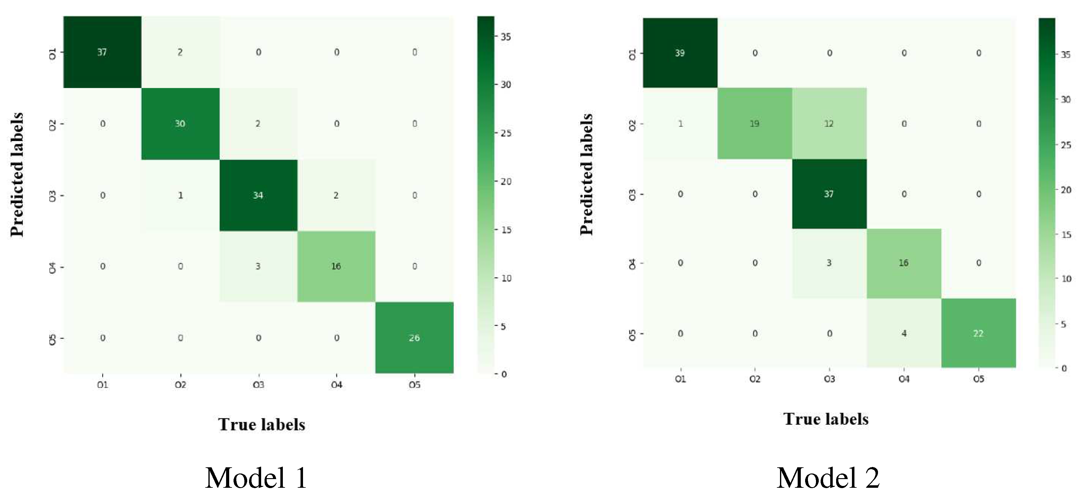
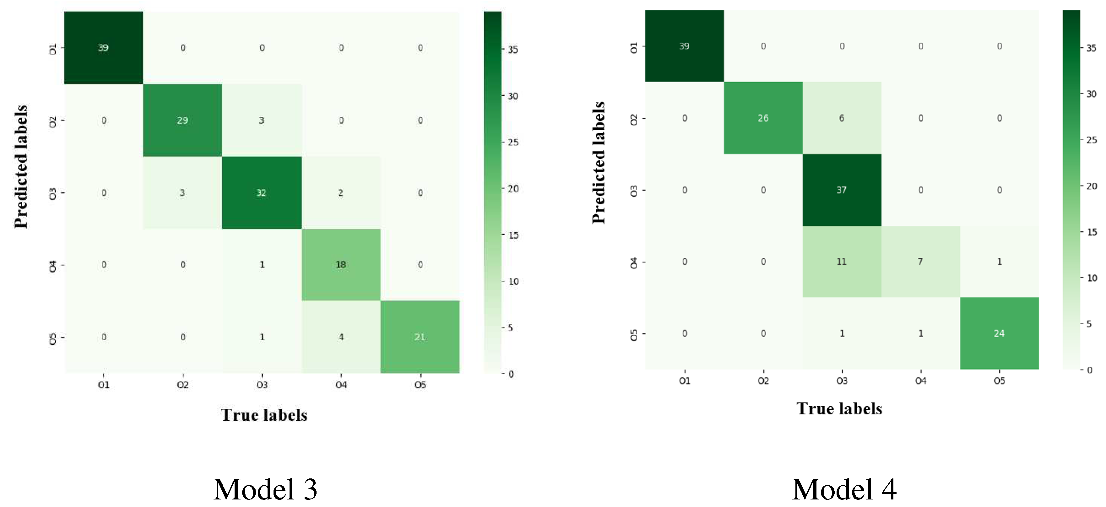
Figure 6 displays the confusion matrices for the classification of five olive classes using four candidate models. The columns represent the true values, while the rows show the predicted values. Upon examining the matrices, we can see that there was only one O1 instance mistakenly classified as O2 using Model 2. The remaining models accurately predicted all O1 instances. Moving on to class O2, one instance was misclassified as O3, and two instances were incorrectly labeled as O1 using Model 1. Additionally, three instances were confused with O3 using Model 3. Models 2 and 4 performed well in predicting class O2, without any mistakes.
Regarding class O3, Model 1 mixed up 3 instances with O4 and 2 instances with O2. Model 2 made similar errors, confusing 3 instances with O4 and 12 instances with O2. Model 3 had a poor performance for this class, mistaking 3, 1, and 1 instances for O2, O4, and O5, respectively. Model 4 also struggled with class O3, confusing 6, 11, and 1 instances with O2, O4, and O5, respectively. For class O4, Model 1 erroneously identified 2 instances as O3, while Model 2 wrongly categorized 4 instances as O5. Model 3 confused 2 and 4 instances with O3 and O5, respectively. Model 4 committed only one mistake, mislabeling an O5 instance as O4. Lastly, in the case of class O5, Models 1, 2, and 3 accurately predicted all instances, while Model 4 mistakenly identified just one O5 instance as O4. In summary, the models generally performed well in recognizing classes O1 and O5, with some inconsistencies in the predictions for classes O2, O3, and O4.
