Unsupervised Wavelet-Feature Correlation Ratio Markov Clustering Algorithm for Remotely Sensed Images

Preprint

Article

Unsupervised Wavelet-Feature Correlation Ratio Markov Clustering Algorithm for Remotely Sensed Images

Altmetrics

Downloads

Views

Comments

A peer-reviewed article of this preprint also exists.

Zhaohui Wang^*

This version is not peer-reviewed

Submitted:

15 November 2023

Posted:

16 November 2023

You are already at the latest version

Alerts

Abstract

The spectrums of one type of object under different conditions have the same features (up, down, protruding, concave) at the same spectral positions, which can be used as primary parameters to evaluate the difference among remotely sensed pixels. Wavelet-feature correlation ratio Markov clustering algorithm (WFCRMCA) for the remotely sensed data is proposed based on an accurate description of abrupt spectral features and an optimized Markov clustering in the wavelet feather space. The peak points can be captured and identified by applying a wavelet transform to spectral data. The correlation ratio between two samples is a statistical calculation of the matched peak point positions on the wavelet feature within an adjustable spectrum domain or a range of wavelet scales. The evenly sampled data can be used to create class centers, depending on the correlation ratio threshold at each Markov step, accelerating the clustering speed by avoiding the computation of Euclidean distance for traditional clustering algorithms, such as K-means and ISODATA. Markov clustering applies several strategies, such as a simulated annealing method and gradually shrinking the clustering size, to control the clustering convergence. At each clustering tempera-ture, it can obtain the best class centers quickly. The experimental results of the Airborne Visible/ Infrared Imaging Spectrometer (AVIRIS) and Thermal Mapping (TM) data have verified its ac-ceptable clustering accuracy and high convergence velocity.

Keywords:

Subject: Computer Science and Mathematics - Artificial Intelligence and Machine Learning

1. Introduction

Identifying suspected targets from remotely sensed data is paramount in everyday life and research. The researchers have extensively investigated numerous clustering algorithms, including cutting-edge technologies, for remotely sensed images, such as Airborne Visible/Infrared Imaging Spectrometer (AVIRIS) and Thermal Mapping (TM) data. However, several limitations exist in these algorithms. One widely used clustering algorithm is K-means clustering, which, unfortunately, cannot automatically determine the number of classes [1,2,3,4]. Moreover, it exhibits slow convergence due to its reliance on minimal spatial distance [5,6].

The approaches ISODATA [7,8] and ISMC [9,10] can determine the class number through self-iteration. Nevertheless, the challenge lies in determining their parameters, particularly in adjusting distance parameters with changing dimensions. On the other hand, orthogonal projection classification suffers from projection fluctuation issues under the restriction of the number of bands [11,12]. Cui introduced a feature extraction method that computes vectorized pixel values from a localized window, enhancing Bag-of-Words (BoW) performance. However, this approach may lead to a reduction in classification accuracy [13,14]. Peng et al. proposed a graph-based structural deep spectral-spatial clustering network to sufficiently explore the structure information among pixels. They designed a self-expression-embedded multi-graph auto-encoder to explore high-order structure associations among pixels, thereby capturing robust spectral-spatial features and global clustering structure [15].

Furthermore, Firat et al. developed a hybrid 3D residual spatial-spectral convolution network to extract deep spatiospectral features using 3D CNN and ResNet architecture [16]. Acharyya combined wavelet theory and neuro-fuzzy techniques for segmentation purposes [17,18]. However, their feature extraction approach solely considers the absolute values of wavelet coefficients, neglecting the specific spectral patterns, and the computational requirements take time and effort.

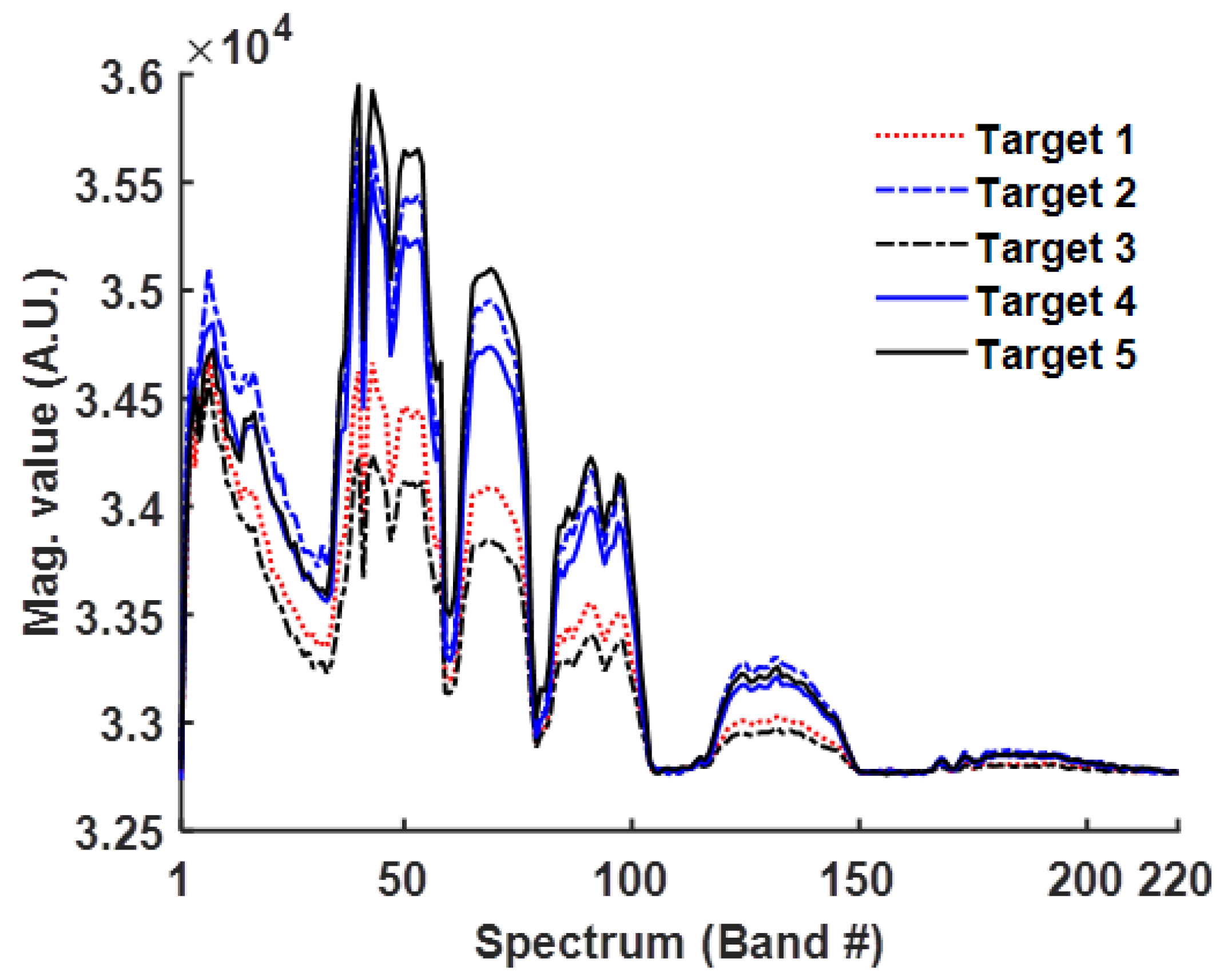
A wavelet-feature correlation ratio Markov clustering algorithm (WFCRMCA) is proposed to differentiate the pixels according to the spectrum similarity between pixels. Of course, the spectrums of one object under different conditions are different. Still, they have the same features (up, down, protruding, concave, see Figure 1) at the same spectral positions, which are the main parameters to evaluate the difference among remotely sensed pixels [19,20]. Therefore, these characteristic positions can denote class features. Fortunately, band-pass wavelet filters can decompose the data at different scales to detect these characteristics.

WFCRMCA can statistically control the clustering accuracy by adjusting parameters such as T_start, T_end, and T_step. A new conception, correlation ratio clustering, is proposed to reflect the similarity between two wavelet-transformed samples. With an accurate description of the abrupt spectral features, wavelet correlation coefficients can differentiate pixels along spectral dimensions. Expanding spectral bands of multi-spectral images increases the number of characteristic points to enrich the features of classes. WFCRMCA forms the clustering space and initial class centers by evenly sampled pixels. Without the initial parameter problem of the K-means algorithm, WFCRMCA can quickly reach the best class centers at each clustering temperature and obtain optimal class centers on the whole scope at high speed by gradually decreasing the clustering scale and temperature. Several theorems are provided and proved to strengthen the WFCRMCA in the Methods section. In the Results section, WFCRMCA receives favorable results for clustering Landsat TM images and AVIRIS hyperspectral images.

2. Methods

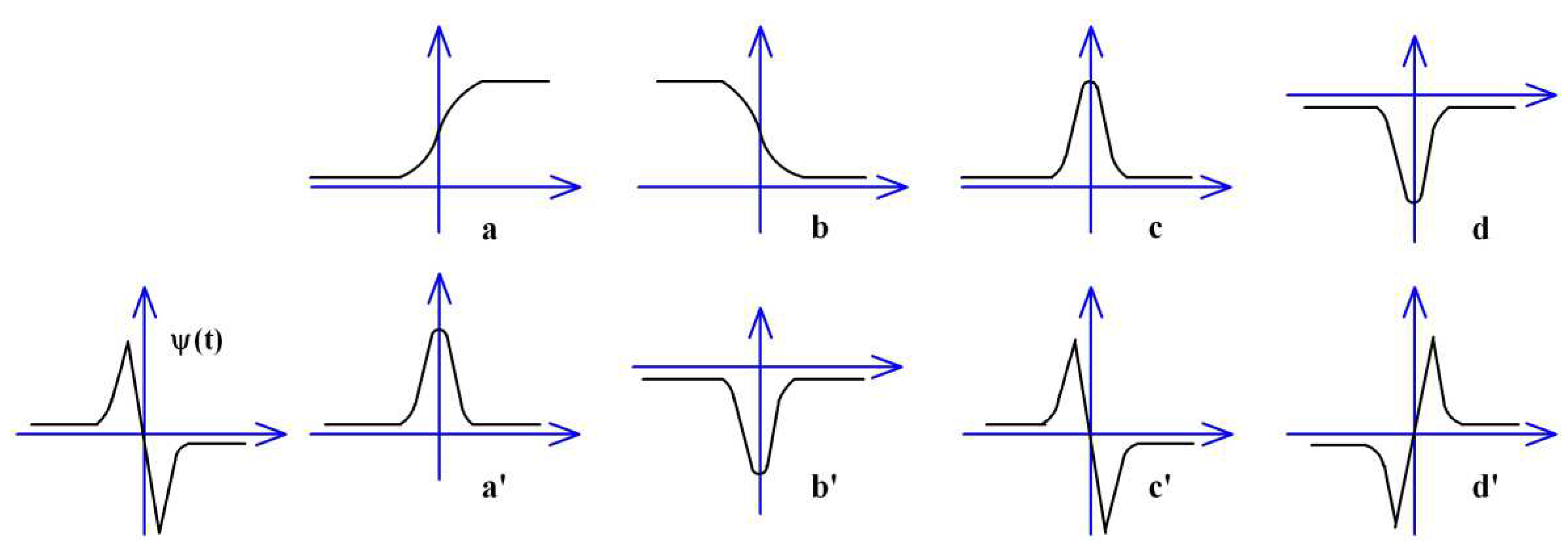
Although the spectral curves of the same objects under different conditions are somewhat different, they have the same feature points (upward, downward, maximum, and minimum) at the same spectral positions (Figure 1). The WFCRMCA could detect abrupt signals through band-pass wavelet transform, such as crossing zero and extreme points. But crossing the zero point cannot be ensured a pulse signal, and perhaps is a smoothly changed signal, so the extreme points between adjacent zero points are much more critical. The signs in spectral vector format are classified according to the priority of importance from low to high: downward, upward, protruding, and concave (Figure 2).

Figure 2 is the result of four kinds of abrupt signals processed by ψ(t) (Equation 1, [21], 1^st derivative Gauss function θ(t)). For some remotely sensed images affected by too many mixed pixels, the position of critical points will probably deviate or have many little fluctuations, so WFCRMCA could eliminate unimportant signals by setting a maximum threshold and only clustering the partial minutia at a high-level scale.

θ (t) = \frac{1}{\sqrt{2 π}} e^{- t^{2} / 2}, ψ (t) = \frac{d θ}{d t} = - \frac{1}{\sqrt{2 π}} t e^{- t^{2} / 2}

(1)

Wavelet feature clustering algorithms only analyze minutia data by detecting and determining the positions of abrupt signals. Using a fast binary Mallet wavelet algorithm [22] in Equation 2 to extract wavelet coefficients, WFCRMCA can mark the upward-maximal points (Figure 2a/a') and downward-minimal points (Figure 2b/b') along the spectrum. WFCRMCA will overlook the weak signals if T_peak is large enough, leading to a failure in identifying some valuable signs among hidden objects.

\{\begin{matrix} c_{j, k} = \sum_{n} h_{n - 2 k} c_{j - 1, n} \\ d_{j, k} = \sum_{n} g_{n - 2 k} c_{j - 1, n} \end{matrix}, j = 1, 2, \dots, S_{c a l e} (\leq ⌊{l o g}_{2} b⌋)

(2)

The WFCRMCA uses r_ij (correlation coefficient, CR), which works like a distance but not Euclidean distance as clustering criteria, to evaluate the difference between two spectral vectors on partial minutia. Equation 3 uses S_cale2-scale minutia of S_cale-scale wavelet coefficients to cluster, t_i,k is the k^th feature of i^th sampled vector, N(·) is the number of feature positions that match criteria. WFCRMCA could use binary values to mark whether the position is valuable enough to attend clustering. When

S_{c a l e 2} = S_{c a l e} = ⌊{l o g}_{2} b⌋

, the bit number attending clustering comparison is

b \sum_{i = 1}^{⌊{l o g}_{2} b⌋} 1 / 2^{i} \approx b - 1

r_{i j} = \frac{N (t_{i, k} = t_{j, k}, k \in Ω)}{N (t_{i, k} \neq t_{j, k}, k \in Ω) + N (t_{i, k} = t_{j, k}, k \in Ω)} i f S_{c a l e 2} = S_{c a l e}, Ω = [0, b \sum_{k = 1}^{S_{c a l e}} \frac{1}{2^{k}} - 1] i f S_{c a l e 2} < S_{c a l e}, Ω = [b \sum_{k = 1}^{S_{c a l e} - S_{c a l e 2}} \frac{1}{2^{k}}, b \sum_{k = 1}^{S_{c a l e}} \frac{1}{2^{k}} - 1]

(3)

2.1. Expanding Bands Method for Multi-spectral Images

As the band number of multi-spectral images (TM images have only seven bands) is not high enough for the wavelet transform to extract efficient feature points, WFCRMCA expurgates the bands with great noise and expands the rest with 2^nd order and nonlinear correlated functions so that WFCRMCA can detect more wavelet features. The expanding multi-spectral bands' method [11] is listed as follows.

Second-order correlated bands include the auto-correlated bands ( ${\{B_{i}^{2}\}}_{i = 1}^{b}$ ) and the cross-correlated bands ( ${\{B_{i} B_{j}\}}_{i, j = 1, i \neq j}^{b}$ ).
Nonlinear correlated bands include the bands stretched out by the square root ( ${\{\sqrt{B_{i}}\}}_{i = 1}^{b}$ ) and those stretched out by the logarithmic function ( ${\{l o g B_{i}\}}_{i = 1}^{b}$ ).

The bands created by 1) and 2), together with the 1^st order bands, which are original (

{\{B_{i}\}}_{i = 1}^{b}

), assemble a new remotely sensed data with (b²+7b)/2 bands.

2.2. Markov Chain Clustering in Wavelet Feature Space

Wavelet-feature Markov clustering algorithm, i.e., WFCRMCA, first denoises the original data to make the spectral features more accurate, then uses a band-pass wavelet filter to detect all dot vectors for sharp points, including upward-maximal and downward-minimal points. As a result, simulated annealing Markov chain decomposition in state space, formed by evenly spatially sampled data, could realize the best centers at each temperature and sub-finest centers on the whole scope.

According to the peculiarity of simulated annealing Markov clustering, each clustering center is one state, and the space is a definite Markov state chain. If two classes (or states) merge, according to CR, it has nothing to do with other states. For example, for Markov chain

I = \{1,2, \dots, n\}

in definite state space

\{X (n)\}

, if any two states communicate, they must be in the same class. Thus, the whole state space (pixels) could be separated into a few isolated classes according to transferred communication. T, which is defined as a threshold value of CR r_ij, is used as an annealing temperature to control the clustering process.

Def. 1

: If

P_{i j}^{1} = r_{i j} - T > 0

for states i and j, they have one-step transferred communication denoted as

i \overset{1}{\leftrightarrow} j

Theorem 1

: Communication can be transferred. If

i \overset{m}{\leftrightarrow} k

and

k \overset{n}{\leftrightarrow} j

(

p_{i k}^{m} > 0, p_{k j}^{n} > 0

i \overset{m + n}{\leftrightarrow} j (p_{i j}^{m + n} > 0)

Proof of Theorem 1.

According to Chapman-Kolmogorov equation:

p_{i j}^{m + n} = \sum_{g ϵ I} p_{i g}^{m} \cdot p_{g j}^{n} \geq p_{i k}^{m} \cdot p_{k j}^{n} > 0 . i . e ., i \overset{m + n}{\leftrightarrow} j .

Def. 2

: If feature i in wavelet characteristic space has p_ij=1, then i is an absorptive state, forming a single-dot set {i}.

Theorem 2.

After Markov clustering, all wavelet features in wavelet feature space are frequently returned states.

Proof of Theorem 2.

i). A single-dot set is an absorptive, frequently returned state.

ii). As simulated annealing clustering causes T to be reduced gradually, the k+1^th clustering iteration is supposed to create a non-single dot set. For instance, m pixels {1, 2,…, m} are absorbed into one class. T^k is the CR threshold of the k^th iteration, and c₁,…, i, … j, …, and c_n are the created clustering centers of the k^th iteration. Thus,

r_{i j} < T^{k}

During the k+1^th iteration,

T^{k + 1} = T^{k} - T_{s t e p}

, where T_step is the depressed step of T at each iteration. If

T^{k + 1} < r_{i j} < T^{k}

, then

p_{i j} = r_{i j} - T^{k + 1} = r_{i j} + T_{s t e p} - T^{k} > 0

and

p_{i j} < T^{k} - T^{k + 1} = T_{s t e p}

, so

i \overset{1}{\leftrightarrow} j

, then i and j are merged together.

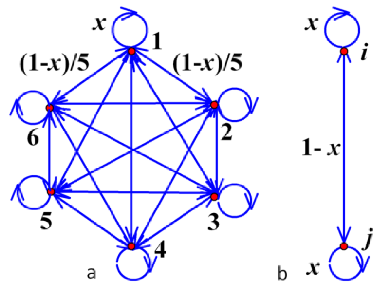
If T_step is small enough (i.e., the temperature is reduced slowly), and i, j, l are absorbed in k+1^th iteration,

p_{i j} = p_{i l} = p_{j l} \approx T_{s t e p}

so that it could be supposed as Figure 3 that

p_{i i} = x, p_{i j} = (1 - x) / (m - 1), i \neq j, i, j \in \{1,2, \dots, m - 1\}

As m states communicate with each other, other m-1 states could be seen as one state j, let p_ii=p_jj=x, p_ij=1-x，thus

f_{i i} = x + {(1 - x)}^{2} + {(1 - x)}^{2} x + \dots + {(1 - x)}^{2} x^{n} + \dots = x + {(1 - x)}^{2} (1 + x + x^{2} + \dots) = 1

So state i is frequently returned state. As m states communicate, the merged m states are frequently returned.

Theorem 3:

The sufficient and necessary condition of closed set C is that, for arbitrary elements

i \in C, j \notin C

, there exists

p_{i j}^{(n)} = 0, n \geq 1

(referring [23,24]).

Theorem 4

: Definite states of Markov chain in wavelet feature space can be uniquely decomposed without overlap into a definite number of frequently returned states, including closed sets C₁, …, C_m and single dot sets C_m+1, …, C_n, existing:

Any two states in C_h $(h ϵ [1, n])$ are communicated.
When $h \neq g$ , $(h, g ϵ [1, n])$ , any state in C_g cannot communicate with any state in C_h (referring [23,24]).

Therefore, every state is frequently returned in the wavelet feature space at each temperature, and the number of isolated closed sets equals the number of classes. Then, the whole wavelet Markov chain feature state space has a decomposable expression that consists of several closed sets without overlap.

2.3. Adjustment of Clustering Centers

When two classes are merged whose correlation ratio r_ij is bigger than T, the numbers of each feature (including crossing zero part) are separately added up at the corresponding position ([0, b-1], the number of wavelet coefficients is approximately b). In addition, their sample numbers are also added up separately.

Similar to the traditional clustering method, reasonable adjustment of clustering centers is based on the statistic of intra-class features. For each position, the feature that occurs most frequently is chosen as the common feature of the new class, and then b common features will be created. If several features come up at the same frequency, the feature with the highest priority (for example, downward-minimal or concave point > upward-maximal or protruding point) is chosen. Then, among all the class centers merged into one new class at this iteration, choose one pixel with the biggest CR with common features as a new class center. According to Equations 4 and 5,

{N B}_{l, k}^{c_{i}}

is the statistic number of feature k on the l^th position in class i,

t^{l}

is the feature of the l^th position, which can be downward (0), upward (1), protruding (2), and concave (3). R(c₁,c₂) is the correlation ratio between vector c₁ and c₂,

Z_{c_{i}}

is the set of class centers absorbed by class i, and

M_{c_{i}}

is the common features of class i.

M_{c_{i}} = \{t^{0} t^{1} \dots t^{b - 1} | {N B}_{l, k}^{c_{i}} > {N B}_{l, j}^{c_{i}}, l \in [0, b - 1], j \neq k, j \in [0,3] \Rightarrow t^{l} = k\}, c_{i} \in C

(4)

\exists x \in Z_{c_{i}}, R (x, M_{c_{i}}) > R (y, M_{c_{i}}), y \neq x, y \in Z_{c_{i}} \Rightarrow c_{i} = x

(5)

During the clustering process, many pixels with high similarity are merged, causing the number of class centers that will attend the following iterative clustering comparison to decrease sharply. As only newly created centers follow next-cycle clustering, WFCRMCA has a high clustering speed.

2.4. Wavelet-Feature Markov Clustering Algorithm

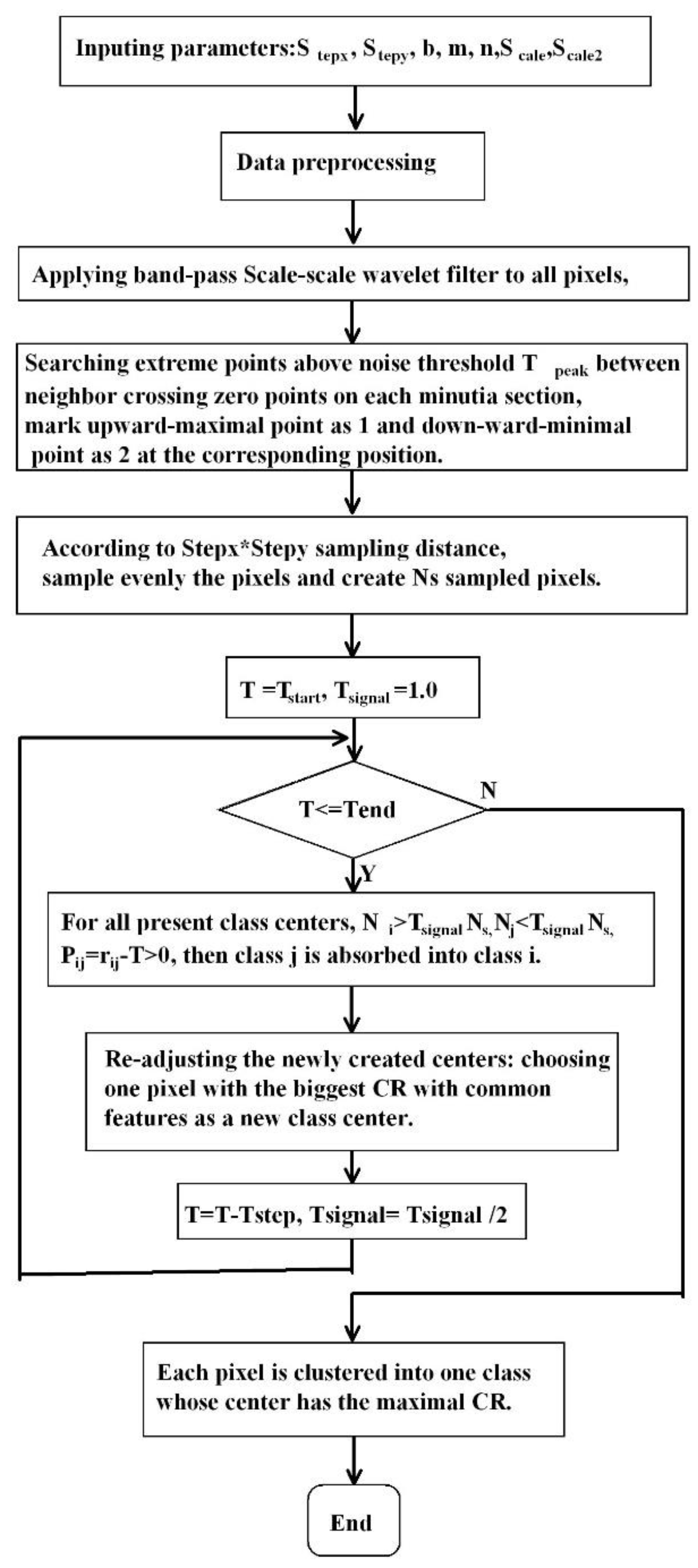
Based on the preceding theoretical analysis, the WFCRMCA uses a simulated annealing technique to gradually decrease CR threshold T through Markov chain decomposition in wavelet feature space at each temperature, obtaining the best clustering centers of the whole space. Supposed that c_i is the class center of class i, S_ci is the pixel set of class i, C is the set of all classes, Z_ci is the set of class centers absorbed by class i at the current temperature, N_c is class number, N_s is the number of sampled pixels (initial class centers are sampled pixels

s_{i}, i \in [0, N_{s} - 1]

), R(c₁,c₂) is the CR between c₁ and c₂,

N (Z_{c_{i}})

is the number of class centers absorbed by class i,

N (S_{c_{i}})

is the pixel number in class i, T_start is the initial value of CR T, and T_end is the lowest CR threshold. The detailed process of WFCRMCA is provided in the flow chart in Figure 4. The simulated annealing Markov chain decomposition clustering in wavelet feature space is listed as follows:

Input parameters:

S_tepx and S_tepy are the sampling distances along horizontal or vertical directions;

b, m, n are separately the band number, column number, and row number of original remotely sensed images;

S_cale is wavelet transform scale;

S_cale2 is the number of minutia scale attending clustering (i.e., S_cale-S_cale2 ~ S_cale minutia sections)

2: Data preprocessing. Delete bands primarily affected by noise and atmosphere, such as the 1-6th, 33rd, 107-114th,153-168th, and 222-224th bands of AVIRIS. Multi-spectral images need to expand bands.
3: Apply band-pass Scale-scale wavelet filter (for example, Equation 6, [25,26]) to all pixels, search extreme points above noise threshold Tpeak between neighbor crossing zero points on each minutia section, and mark upward-maximal point as 1 and downward-minimal point as 2 at the corresponding position.

H = \{0.0,0.125,0.375,0.375,0.125,0.000\}, G = \{- 0.0061, - 0.0869, - 0.5798,0.5798,0.0869,0.0061\}

(6)

4: According to Stepx*Stepy sampling distance, sample the pixels and create Ns sampled pixels evenly.
5: Apply simulated annealing Markov state decomposition clustering to Scale-Scale2~Scale scale minutia sections of sampled data.

a): Set initial temperature T as T_start, the clustering signal standard T_signal (ratio of intra-class sampled pixel number over the number of total sampled pixels) is 1.0, and each pixel is one class center (beginning with N_s class centers). In the end, according to step b-e, apply Markov chain decomposition in state space to the wavelet features of sampled pixels by gradually depressing signal size.

N_{c} = N_{s}, C = \{c_{0}, c_{1}, \dots, c_{N_{c} - 1}\}, S_{c_{i}} = \{s_{i}\}, c_{i} \in C, i \in [0, N_{c} - 1]

(7)

b): Make judgments to all present class centers. If class i is a significant signal in which the number of pixels is more prominent than $T_{s i g n a l} N_{s}$ , move to the next class. Otherwise, search forward one by one for another class j whose size is smaller than $T_{s i g n a l} N_{s}$ , and make clustering judgments between class j and i.
c): According to Equation 8, if the CR between centers of two classes (i and j) meets the condition Pij=rij-T>0, then class j is absorbed into class i. Continuing this process b) until the last class is detected.

Z_{c_{i}} = \{c_{i}\}, c_{i} \in C, \forall c_{i}, c_{i} \in C, i f N (S_{c_{i}}) < T_{s i g n a l} N_{s}, N (S_{c_{j}}) < T_{s i g n a l} N_{s}, R (c_{i}, c_{j}) > T ⟹ {N B}_{l, k}^{c_{i}} = {N B}_{l, k}^{c_{i}} + {N B}_{l, k}^{c_{j}} (l \in [0, b - 1], k \in [0,2]), Z_{c_{i}} = Z_{c_{i}} \cup \{c_{j}\}, S_{c_{i}} = S_{c_{i}} \cup S_{c_{j}}, C = C - \{c_{j}\}, N_{c} = N_{c} - 1

(8)

d): According to Equations 4 and 5, re-adjust the newly created centers: among all the class centers merged into one new class at this iteration, choose one pixel with the biggest CR with common features as a new class center.
e): Let T=T-Tstep decrease clustering temperature, and Tsignal= Tsignal /2 to reduce clustering size. Repeat steps a)-d) until T is reduced to the appointed small signal threshold Tend or set class number is reached.

6: According to the clustering centers created by 5), each pixel is clustered into one class whose center has the maximal CR.

3. Results

The WFCRMCA uses Microsoft Visual C++ language and basic libraries for the code of the proposed algorithm. The TM and AVIRIS data analysis demonstrate the merits and defects of the wavelet feature clustering algorithms, say, WFCRMCA. Classified pixels are shown in white.

3.1. Multi-Spectral Data

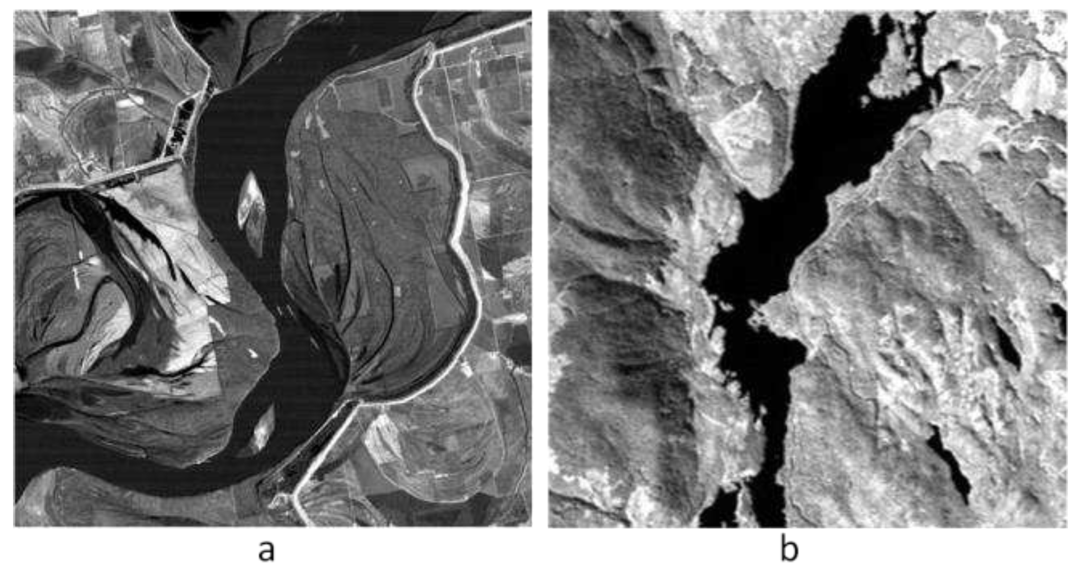
For Mississippi (Figure 5a, 512*512, 8bit, [27]) TM multi-spectral images, the 6^th band heavily affected by the atmosphere is crossed out. The other six bands are expanded to 39: original data: 1-6, second-order auto-correlated bands: 7-12, second-order cross-correlated bands: 13-27, square root function: 28-33, and logarithmic function: 34-39.

It is supposed that T_start=0.95 during the discussion of parameters' influence on Mississippi's clustering results. If only the original six bands are processed by two-scale wavelet decomposition, only four classes are created because features need to be stronger. As the first iteration absorbs too many classes, the intra-class adjustment costs most of the time. The experiment also shows that second-order correlation expanded bands (7^th -27^th) provide more class information, but nonlinear correlation developed bands (28^th-39^th) make the clustering results stable.

The expanding spectrum method increases data processing complexity; however, if there are only several classes, the clustering speed is low because the big class has to spend more time calculating the center. Therefore, this method will keep the clustering speed for multi-spectral data. Table 1 shows that this method could identify the potential specific classes, leading to higher clustering accuracy.

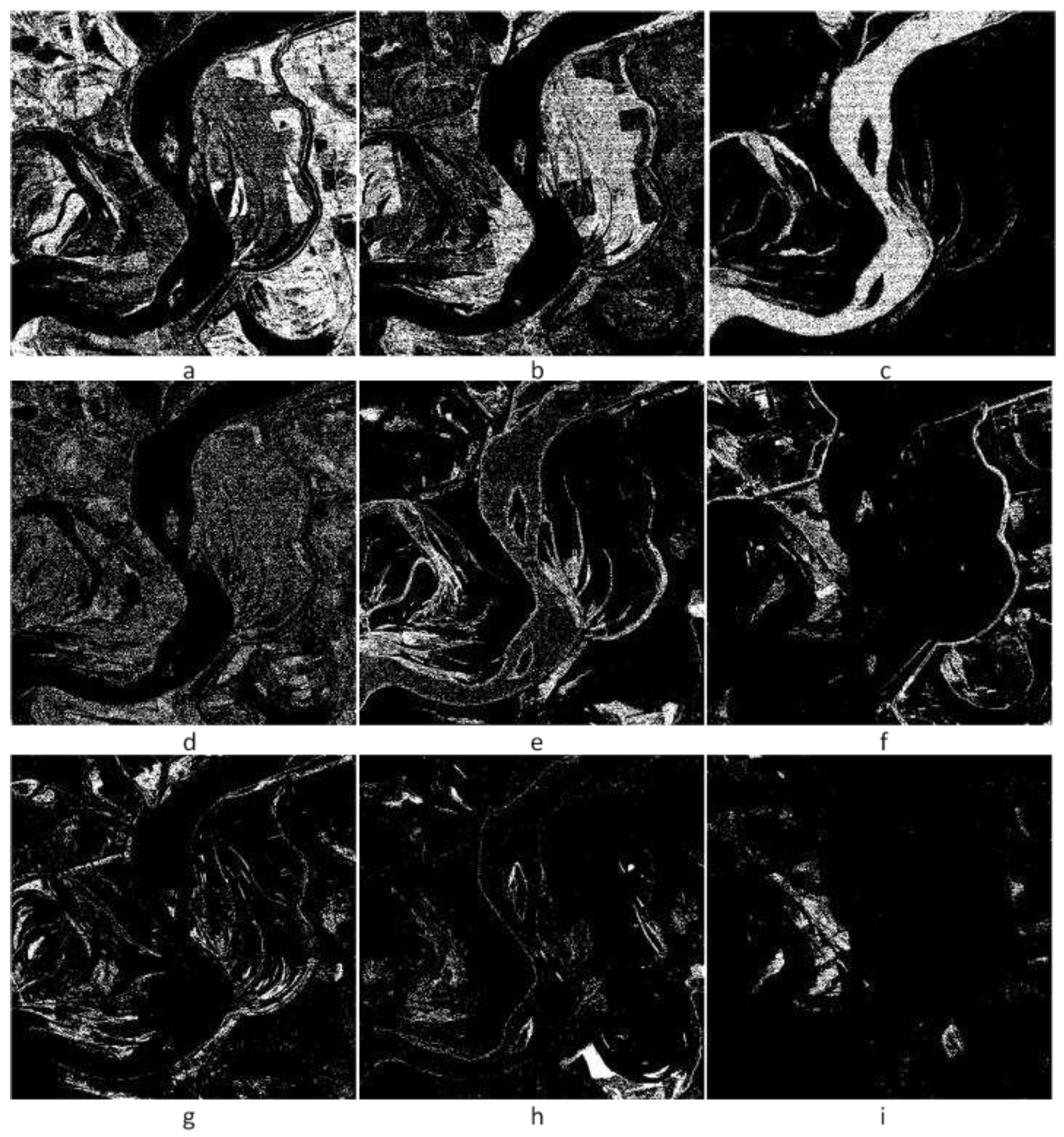
Figure 6 is the clustering result of the parameters in Table 2. It can be seen that class 1 is plow land or meadow (Figure 6a), class 2 is beach (Figure 6b), class 3 is river channel (Figure 6c), class 6 is dyke (Figure 6f), and class 9 is the slope on the bank (Figure 6i). The clustering results maintain significant signals and efficiently embody the minor signs. If the data are divided into 18 classes by the K-means algorithm, one iteration, on average, uses 60 seconds, so this clustering method, according to features on the spectral curves of remotely sensed objects, is more flexible on parameter choice and has quicker clustering speed than standard clustering algorithm (such as K-means).

3.2. Hyper-Spectral Data

For 224 bands Sook Lake (Figure 5b, 256*256, 16bit, [28,29]) AVIRIS hyperspectral images, the WFCRMCA crosses out heavily disturbed bands, such as 1-6^th, 33^rd, 107-114^th, 153-168^th, 222-224^th bands, and use the remaining 190 bands to make algorithm analysis.

In Table 3, when T_peak=0, the number of classes is 133. If T_peak is increased, the number of classes nonlinearly reduces, and clustering time depresses accordingly. When T_peak>7, the number of classes begins to fluctuate, so the WFCRMCA usually chooses T_peak=5.0, which could realize a fairly accurate classification.

In Table 4, with more minutiae attending clustering, the number of clustering classes increases sharply: two of five scale components cluster eight categories; obviously, that does not separate the objects; however, four-scale components cause objects to be dispersed and expand the class number. Depressing T_end could effectively decrease the class number.

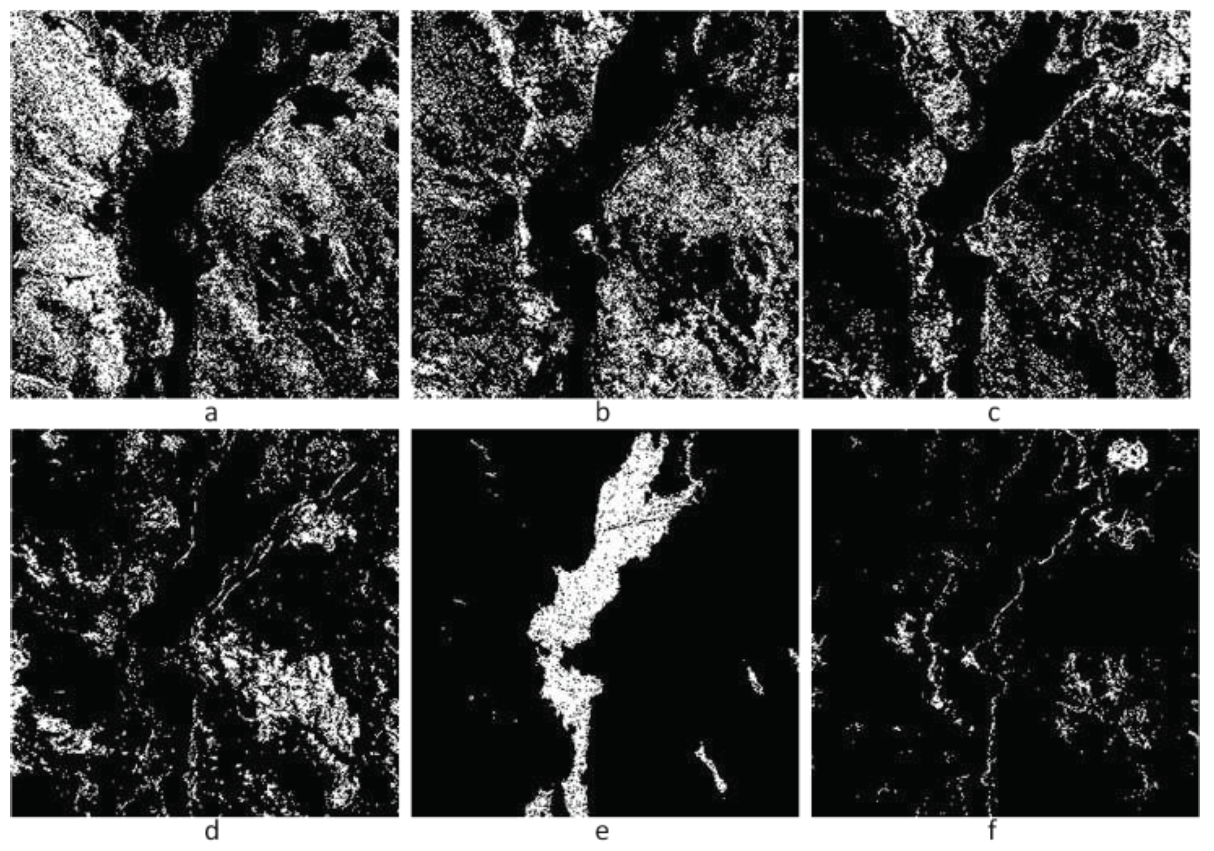
If high three scales of five scales wavelet decomposition are chosen to attend clustering and T_peak=5.0, 17 classes are created (the main clustering results are seen in Figure 7), the time is 21s, division result is favorable; hereinto, class 1 is the basin (Figure 7a), class 4 is for the mountain peaks (Figure 7d), class 5 is the water body of the Sook Lake (Figure 7e).

4. Discussion

For remotely sensed data with a high density of mixed pixels, choosing partial minutia wavelet features in high-level scales could reduce the clustering difficulty caused by a significant amount of minutia, and this also applies somewhat blur to achieve ideal clustering results. Multi-scale classification from fine to coarse could be realized by this method. Furthermore, as the matching speed of abrupt-point positions is very high, clustering time does not increase obviously with the increment of referenced minutia. For example, multi-spectral data typically set S_cale=S_cale2; hyper-spectral data could set S_cale2=S_cale-2.

WFCRMCA applies 1D wavelet transformation on satellite spectral data. Wavelet Transform can represent a signal in both time and frequency domains simultaneously. It decomposes a signal into a set of wavelets that are localized in both time and frequency, allowing me to analyze the signal's time-localized features. Wavelet transform excels at capturing localized features and adaptability to non-stationary signals. However, the Fourier Transform represents a signal in the frequency domain. It decomposes a signal into a sum of sinusoidal components of different frequencies, providing information about the frequency content of the signal. It doesn't capture information about when these frequencies occur. Fourier transform is excellent for spectral analysis.

The ridgelet transformation and curvelet transformation are two well-known methods for high-dimensional image analysis, but the wavelet transformation is better on the 1D spectral feature extraction. In the ridgelet transform, ridgelets are adapted to higher-dimensional singularities; or singularities on curves in dimension two, singularities on surfaces in dimension three, and singularities on (n−1)-dimensional hypersurfaces in dimension n [30]. The curvelet transform uses ridgelet transform as a component step, and it is good at 2D image reconstruction [31]. The proposed WFCRMCA is to use wavelet transform to analyze the 1D spectral data instead of 2D images.

WFCRMCA accelerates clustering speed during the clustering process. The calculation of CR only needs simply matching corresponding characteristic points without the time-consuming floating-point measure of Euclidean distance [1,2]. A great many sampled pixels with high similarity are clustered together during the clustering process, depressing the number of class centers attending clustering comparison; moreover, clustering centers of newly created classes are re-determined according to common features. So, along with the process of this algorithm, the clustering speed continues increasing.

This WFCRMCA only makes statistics of the number of each wavelet feature on every info-position as the class feature and chooses the best pixel as the clustering center but does not directly use the CR matrix to investigate the dependency degree between sampled pixels, resolving spatial complexity problems.

Gradually depressing clustering size could let both small and large signals embody efficiently, and too many noise signals are merged so that the WFCRMCA could detect the spatial position of noise signals.

The WFCRMCA approach can be applied to any spectral data to differentiate targets. It has demonstrated favorable performance for satellite multi-spectral images and super-spectral images. The spectral analysis method can also be used in photoacoustic imaging and OCT.

The WFCRMCA also has several weak points. Even though most parameters are stable and can be used in most cases, several parameters, such as T_peak and S_cale2, still need to be adjusted manually to increase clustering accuracy for specific applications. The Markov clustering method is not parallelizable, though it can provide one optimal solution for clustering the wavelet coefficients at a high convergent velocity. The future work will continue focusing on resolving these issues.

5. Conclusions

The wavelet feature correlation ratio is used to depict the distance between two pixels by analyzing the wavelet features of spectral curves for remotely sensed data. Based on the particularity of CR clustering, a wavelet-feature Markov clustering algorithm is proposed for searching the optimal class centers. After spatial data are evenly sampled, sharp points on the band-pass wavelet coefficients, including extreme points and crossing zero points, are captured and used for clustering matching. WFCRMCA accelerates clustering speed by avoiding the time-consuming Euclidean distance calculation used for general clustering algorithms. For multi-spectral data, nonlinear correlation expanded bands provide more class information than second-order correlation developed bands. Markov clustering based on simulated annealing realizes fast clustering convergence at each temperature.

Funding

This research received no external funding.

Institutional Review Board Statement

Not applicable.

Informed Consent Statement

Not applicable.

Data Availability Statement

The datasets analyzed during the current study are available from the corresponding author upon reasonable request.

Conflicts of Interest

The authors declare no conflict of interest.

References

Wang, Z. Fast multi-level clustering lossless compression algorithm for remotely sensed images, Journal of Image and Graphics 2003, 8(7), pp. 843-848.
Wang, Z.; Zhou, P. Fast clustering lossless compression algorithm for hyperspectral images,” Journal of Remote Sensing 2003, 7(5), pp. 400-406.
Wang, Z. Residual Clustering Based Lossless Compression for Remotely Sensed Images, 2018 IEEE International Symposium on Signal Processing and Information Technology (ISSPIT), Louisville, KY, USA, 2018, pp. 536-539. [CrossRef]
Wang, Z. Entropy Analysis for Clustering Based Lossless Compression of Remotely Sensed Images," 2021 IEEE International Conference on Big Data (Big Data), Orlando, FL, USA, 2021, pp. 4220-4223. [CrossRef]
Theodoridis, S.; Theodoridis, S.; Koutroumba, K. Pattern Recognition, 4^th ed; Academic Press: Cambridge, MA, USA, 2008; pp. 741-745.
Ikotun, A. M.; Ezugwu, A. E.; Abualigah, L.; Abuhaija, B.; Heming, J. K-means Clustering Algorithms: A Comprehensive Review, Variants Analysis, and Advances in the Era of Big Data. Information Sciences 2023, 622, pp. 178-210. [CrossRef]
Soto de la Cruz, R.; Castro-Espinoza, F. A.; Soto, L. Isodata-Based Method for Clustering Surveys Responses with Mixed Data: The 2021 StackOverflow Developer Survey. Computación y Sistemas 2023, 27(1), pp. 173-182. [CrossRef]
Arai, K. Improved ISODATA Clustering Method with Parameter Estimation based on Genetic Algorithm. International Journal of Advanced Computer Science and Applications 2022, 13(5), pp. 187-193. [CrossRef]
Simpson, J. J.; McIntre, T. J.; Sienko, M. An Improved Hybrid Clustering Algorithm for Natural Scenes. IEEE Trans. Geosci. Remote Sensing 2000, 38(2), pp.1016-1032. [CrossRef]
Bo, L.; Bretschneider, T. D-ISMC: A distributed unsupervised classification algorithm for optical satellite imagery. In Proceedings of the 2003 IEEE International Geoscience and Remote Sensing Symposium, (July 2003), Vol. 6, pp. 3413-3419.
Ren, H.; Chang, C.-I. A Generalized Orthogonal Subspace Projection Approach to Unsupervised Multi-spectral Image Classification. IEEE Trans. Geosci. Remote Sensing 2000, 38(6), pp.2515-2528.
Ifarraguerri, A.; Chang, C.-I. Unsupervised Hyperspectral Image Analysis with Projection Pursuit. IEEE Trans. Geosci. Remote Sensing 2000, 38(6), pp.2529-2538. [CrossRef]
Cui, S.; Schwarz, G.; Datcu, M. Remote sensing image classification: No features, no clustering. IEEE Journal of Selected Topics in Applied Earth Observations and Remote Sensing 2015, 8(11), pp. 5158-5170.
Chen, X.; Zhu, G.; Liu, M. Bag-of-Visual-Words Scene Classifier for Remote Sensing Image Based on Region Covariance. IEEE Geoscience and Remote Sensing Letters 2022, 19, pp. 1-5. [CrossRef]
Peng, B.; Yao, Y.; Lei, J.; Fang, L.; Huang, Q. Graph-Based Structural Deep Spectral-Spatial Clustering for Hyperspectral Image. IEEE Transactions on Instrumentation and Measurement 2023 (accepted). [CrossRef]
Firat, H.; Asker, M. E.; Bayindir, M. I.; Hanbay, D. 3D residual spatial–spectral convolution network for hyperspectral remote sensing image classification. Neural Computing and Applications 2023, 35(6), pp. 4479-4497. [CrossRef]
Acharyya, M.; De, R. K.; Kundu, M. K. Segmentation of remotely sensed images using wavelet features and their evaluation in soft computing framework. IEEE Trans. Geosci. Remote Sensing 2003, 41(12), pp. 2900-2905.
Anupong, W.; Jweeg, M. J.; Alani, S.; Al-Kharsan, I. H.; Alviz-Meza, A.; Cárdenas-Escrocia, Y. Comparison of Wavelet Artificial Neural Network, Wavelet Support Vector Machine, and Adaptive Neuro-Fuzzy Inference System Methods in Estimating Total Solar Radiation in Iraq. Energies 2023, 16, 985. [CrossRef]
Wang, Z.; Zhou, P. Greedy clustering algorithm and its application for the classification and compression of remotely sensed images, Jounal of University of Science and Technology of China 2003, 33(1), pp. 52-59.
Wang, Z.; Zhou P. Fast clustering based on spectral wavelet features extraction and simulated annealing algorithm for multi-spectral Images, Journal of Image and Graphics. 2002, 7A(12), pp. 1257-1262.
Haddad, S. A. P.; Serdijn, W. A. Ultra low-power Biomedical Signal Processing: An Analog Wavelet Filter Approach for Pacemakers, Springer Science & Business Media: Berlin, Germany, 2009; pp. 34-50.
Mallat, S.G. A theory for multiresolution signal decomposition: The wavelet representation. IEEE Trans. Pattern Anal. Mach. Intell. 1989, 11, pp.674–693. [CrossRef]
Joseph, A. Markov Chain Monte Carlo Methods in Quantum Field Theories: A Modern Primer. Springer Nature, 2020; pp. 29-35.
Bittelli, M.; Olmi, R.; Rosa, R. Random Process Analysis With R; Oxford University Press, 2022; pp. 25-31.
Li, Q.; Zhao, J.; Zhao, Y.-N. Detection of Ventricular Fibrillation by Support Vector Machine Algorithm. IEEE International Asia Conference on Informatics in Control, Automation and Robotics 2009, pp. 287-290.
Swelends, W. The Lifting Scheme: A Custom-design Construction of Biorthogonal Wavelet. Journal of Appl. And Comput. Harmonic Analysis 1996, 3(2), pp. 186-220.
Kulkarni, A.; McCaslin, S. Knowledge Discovery from Multi-spectral Satellite Images. IEEE Geosci. Remote Sens. Lett. 2004, 1(4), pp. 246-250,.
Goodenough, D. G.; Bhogal, A. S.; Dyk, A.; Niemann, O.; Han, T.; Chen, H.; West, C.; Schmidt, C. Calibration of Forest Chemistry for Hyperspectral Analysis. In IEEE 2001 International Geoscience and Remote Sensing Symposium 2001, 1, pp. 52-56.
Goodenough, D. G.; Dyk, A.; Niemann, K. O.; Pearlman, J. S.; Chen, H.; Han, T.; Murdoch, M.; West, C. Processing Hyperion and ALI for Forest Classification. IEEE Trans. Geosci. Remote Sensing 2003, 41(6), pp. 1321-1331. [CrossRef]
Candès, E. J.; Donoho, D. L. Ridgelets: A key to higher-dimensional intermittency? Philosophical Transactions of the Royal Society of London. Series A: Mathematical, Physical and Engineering Sciences 1999, 357(1760), 2495-2509.
Starck, J. L.; Candès, E. J.; Donoho, D. L. The curvelet transform for image denoising. IEEE Transactions on image processing 2002, 11(6), pp. 670-684. [CrossRef]

Disclaimer/Publisher’s Note: The statements, opinions, and data contained in all publications are solely those of the individual author(s) and contributor(s) and not of MDPI and/or the editor(s). MDPI and/or the editor(s) disclaim responsibility for any injury to people or property resulting from any ideas, methods, instructions, or products referred to in the content.

Figure 1. Five points at different spatial positions within the same class have the same features at the exact spectral locations.

Figure 2. The wavelet band-pass filter and four kinds of abrupt signals. a-d are the four critical signals: upward-maximal point, downward-minimal point, protruding crossing zero point, and concave crossing zero point. ψ(t) is the band-pass wavelet filter, a’-d’ are the output of the four signals through the wavelet filter.

Figure 3. Closed set composed of five class centers.

Figure 4. Flow chart of WFCRMCA.

Figure 5. (a) Mississippi TM 4th band image after gray balance. (b) Sook Lake AVIRIS 60^th band image after gray balance.

Figure 6. Mississippi TM image, WFCRMCA clustering results: (a)-(i) are the eight significant signals.

Figure 7. Sook Lake AVIRIS image WFCRMCA clustering result. a-f are the seven significant signals.

Table 1. Expanded bands number comparison (3*3 sampling, S_cale = S_cale2 =5,T_signal=0.1,T_step=0.01).

Band number	T_cr1	T_cr2	Class number
6(S_cale=2)	0.8	0.8	4
39	0.7	0.7	36

Table 2. Mississippi TM clustering (sampling 5*5, S_cale =4, T_peak=5, T_start =0.9,T_step=0.05).

Band no.	T_cr1	T_cr2	S_cale2	Class no.
39	0.9	0.4	4	18

Table 3. Sook lake AVIRIS hyper-spectral image, WFCRMCA clustering parameter T_peak comparison (5*5 sampling, band number 190, S_cale=5, S_cale2=4, T_start=0.9, T_step=0.05).

T_peak	T_end	Class number
0	0.4	133
2	0.4	65
5	0.4	38
7	0.4	26
10	0.4	22
15	0.4	24

Table 4. Sook lake AVIRIS hyper-spectral image WFCRMCA clustering parameters T_end and S_cale2 comparison (5*5 sampling, band number is 190, S_cale =5, T_peak=5, T_start =0.9, T_step=0.05).

T_end	S_cale2	Class number	Time/sec.
0.4	2	8	13
0.4	3	17	21
0.4	4	38	51
0.6	4	85	52

Disclaimer/Publisher’s Note: The statements, opinions and data contained in all publications are solely those of the individual author(s) and contributor(s) and not of MDPI and/or the editor(s). MDPI and/or the editor(s) disclaim responsibility for any injury to people or property resulting from any ideas, methods, instructions or products referred to in the content.

© 2023 by the authors. Licensee MDPI, Basel, Switzerland. This article is an open access article distributed under the terms and conditions of the Creative Commons Attribution (CC BY) license (http://creativecommons.org/licenses/by/4.0/).

Copyright: This open access article is published under a Creative Commons CC BY 4.0 license, which permit the free download, distribution, and reuse, provided that the author and preprint are cited in any reuse.

MDPI Initiatives

Important Links

Choose an area of interest and we will send you notifications of new preprints at your preferred frequency.

Disclaimer

Unsupervised Wavelet-Feature Correlation Ratio Markov Clustering Algorithm for Remotely Sensed Images

Abstract

1. Introduction

2. Methods

2.1. Expanding Bands Method for Multi-spectral Images

2.2. Markov Chain Clustering in Wavelet Feature Space

2.3. Adjustment of Clustering Centers

2.4. Wavelet-Feature Markov Clustering Algorithm

3. Results

3.1. Multi-Spectral Data

3.2. Hyper-Spectral Data

4. Discussion

5. Conclusions

Funding

Institutional Review Board Statement

Informed Consent Statement

Data Availability Statement

Conflicts of Interest

References

MDPI Initiatives

Important Links

Subscribe