
You are currently viewing a beta version of our website. If you spot anything unusual, kindly let us know.
Preprint
Article
Machine Learning Application to Brain Diseases Detection
Altmetrics
Downloads
103
Views
222
Comments
0


This version is not peer-reviewed
Abstract
During a multi-detector computed tomography (MDCT) examination, it is crucial to efficiently organize, store, and transmit medical images in DICOM standard, which requires significant hardware resources and memory. Our project processed large amounts of DICOM images by classifying them based on cross-section views that may carry important information about a possible diagnosis. We ensured that images were retained and saved in PNG format to optimize hardware resources while preserving patient confidentiality. Furthermore, we have developed a graphical, user-friendly interface that allows physicians to visualize specific regions of interest in a patient's brain where changes may indicate disease. Our proposed method enables quick classification of medical images into predefined classes of confirmed diseases of brain parenchyma, contributing to swift decision-making for further diagnosis for more precisely evaluating and characterizing brain changes, and it can lead to the rapid application of adequate therapy, which may result in better outcomes.
Keywords:
Subject: Computer Science and Mathematics - Artificial Intelligence and Machine Learning
1. Introduction
In the scientific literature, many models have been proposed for detecting various brain diseases in patients. The Smart Visualization of Medical Images (SVMI) method [1], proposed in 2022, enables innovative visualization of medical images as a tool in the function of education in neuroradiology relevant to medical imaging research and provides a valuable tool for analyzing medical images.
Detecting brain diseases is a critical task that can be made easier and more accurate using artificial intelligence (AI) and machine learning (ML). By analyzing large amounts of data, ML algorithms can identify patterns and anomalies that may be difficult for humans to detect. This can lead to earlier and more accurate diagnoses and better patient outcomes. Myszczynska et al. [2] discuss how machine learning as a subfield of artificial intelligence can aid early diagnosis and interpretation of medical images and the discovery and development of new therapies. Najjar [3] shed light on AI applications in radiology, elucidating their seminal roles in image segmentation, computer-aided diagnosis, predictive analytics, and workflow optimization while fostering robust collaborations between specialists in the field of radiology and AI developers.
Segmentation and classification of medical images represent essential techniques for detecting various brain diseases and critical decision-making processes for the timely application of the right therapy. Precise segmentation of medical images of the brain brings valuable information to physicians for disease diagnosis, application of adequate therapy, and further pharmacological or surgical procedures. As a critical task, segmentation and classification of medical images involves separating an image into multiple regions, or segments, based on its features and characteristics and then classifying those segments into different categories. This process is used in various medical applications, such as disease diagnosis, treatment planning, and medical research. In the scientific and research literature, image segmentation and classification tasks include various approaches for disease detection on most organs in the human body. Kim et al. [4] have developed an AI model for estimating the amount of pneumothorax on chest radiographs using U-net that performed semantic segmentation and classification of pneumothorax and areas without pneumothorax. Balasubramanian et al. [5] apply a novel model for segmenting and classifying liver tumors built on an enhanced mask region-based convolutional neural network (R-CNN mask) used to separate the liver from the computed tomography (CT) abdominal image, with prevention of overfitting, the segmented picture is fed onto an enhanced swin transformer network with adversarial propagation (APESTNet). Sousa et al. [6] investigated the development of a deep learning (DL) model, whose architecture consists of the combination of two structures, a U-Net and a ResNet34. Primakov et al. [7] present a fully automated pipeline for the detection and volumetric segmentation of non-small cell lung cancer validated on 1328 thoracic CT scans from 8 institutions. Li Kang et al. [8] propose a reference-based framework to assess the image-level quality for overall evaluation and pixel-level quality to locate mis-segmented regions. In their work, Li Kang et al. proposed a reference-based framework to conduct thorough quality assessments on cardiac image segmentation results for reliable computer-aided cardiovascular disease diagnosis. Li Rui et al. [9] gave a review that focuses on segmentation and classification parts based on lung nodule type, general neural network and multi-view convolutional neural network architecture. Ruffle et al. [10] present brain tumor segmentation with incomplete imaging data based on magnetic resonance imaging (MRI) of 1251 individuals, where they quantify the comparative fidelity of automated segmentation models drawn from MR data, replicating the various levels of completeness observed in real life. Ghaffari et al. [11] developed an automated method for segmenting brain tumors into their sub-regions using an MRI dataset, which consists of multimodal postoperative brain scans of 15 patients who were treated with postoperative radiation therapy, along with manual annotations of their tumor sub-regions. Gaur et al. [12] used an explanation-driven dual-input CNN model to find if a particular MRI image is subjected to a tumor or not and used a dual-input CNN approach to prevail over the classification challenge with images of inferior quality in terms of noise and metal artifacts by adding Gaussian noise.
The scientific works mentioned above are only a glimpse of insight into recent literature. Many of the mentioned works and scientific research, with the application of advanced machine learning algorithms, can obtain accurate and reliable results, leading to better patient outcomes and more effective treatments. In neuroradiology, in the analysis of medical images by physicians and specialists, certain obstacles make it difficult or impossible to visualize and interpret the findings adequately. Disturbances are reflected as artifacts that mimic pathology, degrade image quality, and can occur due to patient movement during imaging or previous surgical or interventional radiologist procedures. Difficulties in recognizing and segmenting medical images of patients' brains can also be reflected in other noises, such as the poor resolution of the device during setup or beam hardening caused by the presence of a metal element in the patient's body that makes it difficult for the device's beam to penetrate the patient. Zheng et al. [13] have emphasized the significance of accurately processing medical images affected by solid noise and geometric distortions, as it plays a crucial role in clinical diagnosis and treatment. The limitations of grayscale images, such as poor contrast and the complexity of medical images obtained from MDCT and MRI devices, with individual variability, make MR brain image segmentation a challenging task. Jiang et al. [14] proposed a distributed multitask fuzzy c-means clustering algorithm that shows promise in improving the accuracy of MR brain image segmentation. This algorithm extracts knowledge among different clustering tasks. It exploits the standard information among different but related brain MR image segmentation tasks, thus avoiding the adverse effects caused by noisy data existing in some MR images.
In recent years, there have been significant advancements in the field of machine learning for medical image processing. Application of deep learning techniques, such as convolutional neural networks (CNNs) and recurrent neural networks (RNNs), medical images can now be analyzed and interpreted with greater accuracy and efficiency. These advancements have the potential to revolutionize medical diagnosis and treatment, as they enable healthcare professionals to detect and diagnose diseases earlier and with higher precision. These advancements have enabled accurate classification of medical images obtained from various devices and apparatus. Long et al. [15] adapted contemporary classification networks into fully convolutional networks and transferred their learned representations to detailed segmentation of brain cancer. In their study, Hu Mandong et al. [16] introduced a model that utilizes improved fuzzy clustering to predict brain disease diagnosis and process medical images obtained from MRI devices. They incorporated several techniques, including CNN, RNN, Fuzzy C-Means (FCM), Local Density Clustering Fuzzy C-Means (LDCFCM), and Adaptive Fuzzy C-Means (AFCM), in simulation experiments to compare their performance. As convolutional neural networks are a widely used deep learning approach to the brain tumor diagnosis, Xie et al. [17] present a comprehensive review of studies using CNN architectures for the classification of brain tumors using MR images to identify valuable strategies and possible obstacles in this development. Salehi et al. [18] analyze the importance of CNN improvements in image analysis and classification tasks and review the advantages of CNN and transfer learning in medical imaging, including improved accuracy, reduced time and resource requirements, and the ability to resolve class imbalance. Despite the significant progress in developing CNN algorithms, Mun et al. [19] proposed areas for improvement for the future radiology diagnostic service.
In this paper, we present innovative approach to analyzing medical images during a multi-detector computed tomography (MDCT) examination.
2. Methods and Results
Artificial intelligence, machine learning, and deep learning models give excellent results in terms of classification. However, most models are considered as “black boxes” [20,21]. It is necessary for a specialist to extract essential features of the image based on the part of the image that contains valuable information, excluding pixel values that contain irrelevant information for decision-making (background, bones, and medical apparatus).
2.1. DCM to PNG Conversion
For a multi-detector computed tomography (MDCT) examination, it is crucial to efficiently organize, store, and transmit medical images in DICOM standard (Digital Imaging and Communications in Medicine, a DCM extension), which requires significant hardware resources and memory.
During his work, a physician specialist encounters rare and different diseases that are represented in an atypical way. For this purpose, during his continuous learning, he consults current scientific research achievements to improve his knowledge, compares his opinion with the development of expertise in neuroradiology, and provides an adequate differential diagnosis. For this purpose, in the first step of our implemented model, medical images were downloaded from the Internet to test the software and establish the result in consultation with the knowledge of a neuroradiology physician specialist built up over decades of learning.
More than 400,000 medical images in DCM format containing 512×512 pixels were downloaded from the Internet [22]. MDCT scanning was made on different devices with a vast difference in values and different offsets for the black level, i.e., the background. The medical images contain 512×512 pixels, a total of 262,144 pixels, each with at least 2 bytes of data; approximately 513 KB ≈ 0.5 MB of footprint for each image.
The first problem is that all downloaded medical images are in DCM format, each occupying 0.5 MB of memory space. Downloaded images require a storage space of ≈ 400,000×0.5 MB, approximately 200,000 MB, or 200 GB. Although patient data is hidden on downloaded images, hiding or deleting private data on new medical images from MDCT scanning is highly important.
To avoid the appearance of private data on medical images and to maintain the correct and exact pixel values, the PNG format (Portable Network Graphics) was chosen for saving, distributing, and sharing images. From the DCM format, the footage loads only the pixel value data and not the metadata into the software package. The images are then saved in PNG format, which is, on average, four times smaller or about 135 KB, with size variations in memory from 1 KB to 200 KB. Some PNG images were immediately deleted because their size was so small that they did not contain useful information. These were images less than 10 KB in size. By converting the DCM format to the PNG format, we reduced the usage of the computer memory from 200 GB to 70 GB.
After generating the PNG images, the DCM images can be deleted. The entire process of converting footage from DCM format to PNG, saving footage in PNG format, and then deleting footage in DCM format is automated. In addition to reducing the large memory hardware requirement for storing DCM images from 200 GB to PNG images (70 GB), the software is faster because it uses less memory to process the images.
The next goal is to review medical images from the Internet in a simplified and efficient way and to separate those with potentially helpful content corresponding to the images the specialist is currently interested in. They are black-and-white images with shades of gray and appropriate textures that show the brain parenchyma. This is especially important in cases of rare diseases or those that do not have typical representations.
By deleting the DICOM format and generating the PNG format, we reduce disk (memory) usage and possibly faster exchange of images because the images obtained by conversion are at least four times smaller. The accuracy of the pixels that carry the image information is not reduced. Also, by converting images from DICOM format to PNG, we ensure the privacy of patient, physician, and institution data, and we do further processing with PNG format.
2.2. Adjusting Pixel Values in the Visible Range
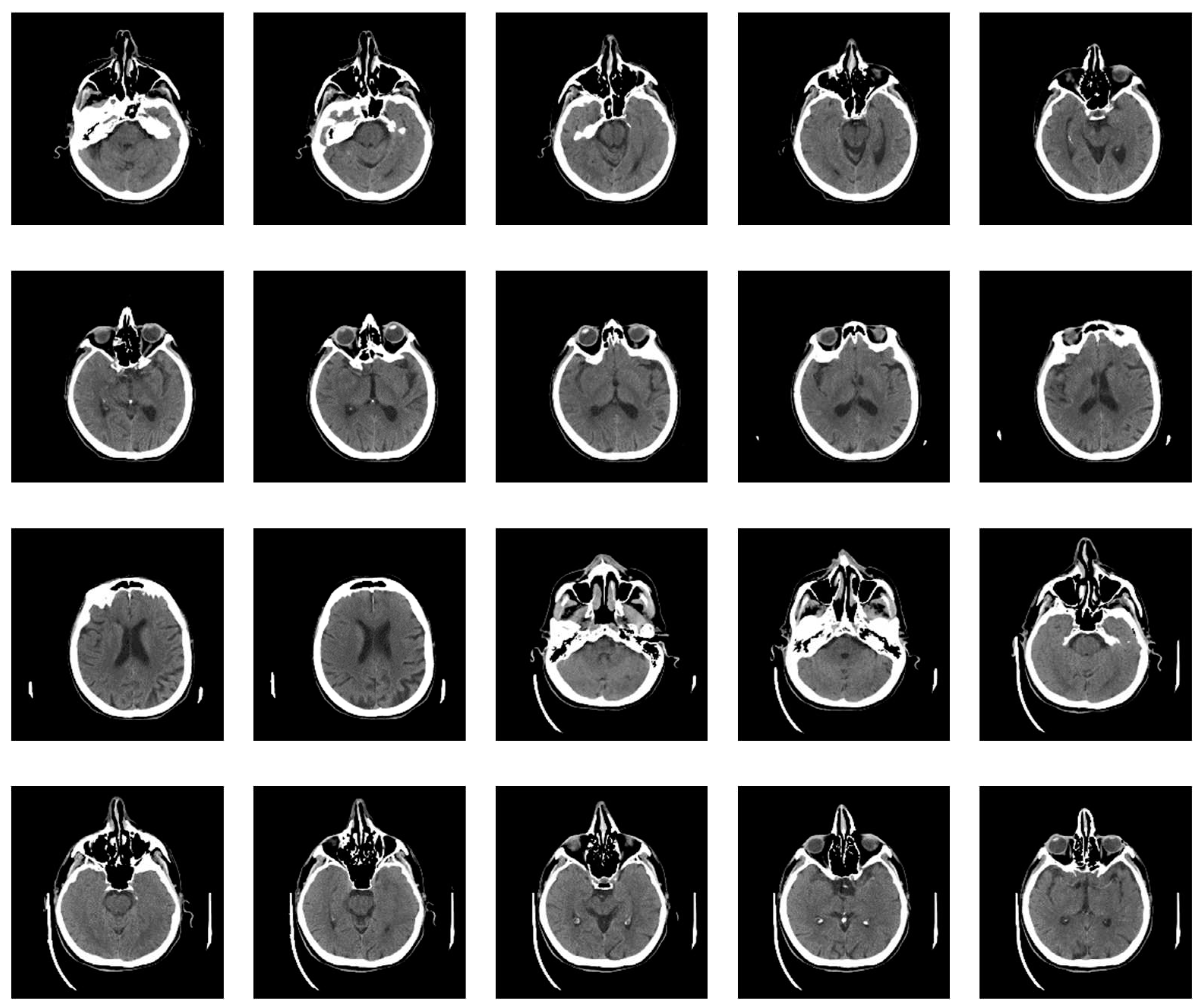
In this phase stage, based on the reviewed 400 images (0.1% of those downloaded from the Internet), we observed five characteristic classes (Figure 1): (a) Nothing – the content of the image is small illuminated parts in the central part of the image; (b) Something – class cannot be determined; (c) Empty – uniform content without parenchyma texture; (d) Bones – the part that contains the bones expressed in the central part of the image; and under (e) Visible – the part that looks like something that physician specialists would be interested in because it shows brain parenchyma that could indicate disease in further analysis. Examples of images of characteristic classes are shown in Figure 1.
The next step in our method is to process the images with applied functions so that the contents of the images are similar for classification because the images were made on different medical devices and apparatus, on which the pixel values differ drastically. Our applied method introduces non-linear distortions so that the pixels with large values and few are compressed. At the same time, the many dark pixels are also compressed so that the pixels that should carry information in the brain parenchyma rescale to the maximum range from 0 to 1. Now, the specialist has formed groups of images to train the software for further analysis. All images were obtained using the command for adjusting pixel values so that more of the image content is in the visible range or to correct lousy illumination or contrast, i.e., ImageAdjust. This highlights the part that contains valuable information and normalization independent of the image generation method. The images are in shades of gray with a range of values from 0 to 1. The specialist selects typical representatives of the classes of his choice and places them in lists (an example of representative classes is shown in the following Figure 2).
All selected images are saved in a unique folder, Samples. The analysis software loads the images from the Samples folder without displaying them on the screen to keep the working file small; otherwise, the working file can become very large, which may affect the proper operation of the software. By converting images to a smaller format with ImageAdjust, the software can work with smaller files, which further speeds up further processing, for example, image classification. ImageAdjust's correction transformation is applied to each pixel value, using S transformation or cropping [23] (represented in the following Figure 3).
In our software, we are using a similar transformation by clipping very large or small pixel values.
2.3. Classification of a Massive Number of Medical Images
Machine learning as a subfield of artificial intelligence solves the problems of classification, clustering, and forecasting complex algorithms and methods, with the ability to extract patterns from raw data [24,25,26]. Also, deep learning is used in linear systems analysis [27,28]. In most cases, machine learning uses supervised learning [29]; the computer learns from a set of input-output pairs, which are called labeled examples. Classification of medical images requires an expert, which in our case is a physician specialist. In classifying medical images, a specialist who has generalized five classes applies a classifier based on labeled examples, a set of input/output pairs: imgEBTNSV = Classify[{imgN0[[1]] -> "Nothing", imgB0[[2]] -> "Bones", imgV0[[3]] -> "Visible", imgE0[[1]] -> "Empty", imgV0[[2]] -> "Visible",...}];.
After the specialist assigns a text to the selected images with a description of the meaning of the image display, the images from the work folder are classified. Each image is copied to the appropriate folder and deleted in the working directory. Because of the preparation of images that are now, after conversion, relatively small, it takes about 0.1 seconds to process one image. The whole process is performed automatically to sort all images by class. For 397,994 medical images, the conversion and sorting process takes about a day. For images downloaded from the Internet, the classifier sorted the following classes: Empty 42.2%, Nothing 27.4%, Bones 10.6%, Visible 10.1%, and Something 9.7%. It is important to note that the result depends on the specialist's choice of which medical images he assigned which text as the class description.
Since the specialist chose a small set of images, should be expected to be some classes overlap. Even if the specialist had taken a more extensive set of images, classes would overlap. Therefore, whether the classification is correct and the samples are appropriately chosen should be checked. As the classifier classified about 10% of the images as Visible, about 40,000, the specialist again assigns images to samples from this set of 40,000 for additional sorting. Processing 40,000 images now takes about a couple of hours. The result of execution is that the Visible is 0.9%, Bones 22.1%, Empty 59.5%, Nothing 13.0%, and Something 4.5%. According to the sample selection criteria, the Visible class now contains 350 images that could have valuable content. With a further procedure, it is no longer necessary to use machine learning because a specialist can sort several hundred images by visual inspection of all. Of course, the whole procedure is automated so that the specialist can use the GUI (presented in Figure 4).
In the first step, the specialist selects the image (Figure 4a) and the file name containing that image (Figure 4b) and can decide which class image belongs. In the tab, each class is visually represented by a symbol in order from top to bottom (shown in Figure 4c): x for Nothing; ρ for Bones; 0 for Empty; ? for Something; and √ Visible. The specialist chooses the class according to the marks, so if he chooses the last class marked with the symbol √ (Checkmark symbol), he decides that the image may contain useful information.
After copying to a subfolder, the file should be deleted from the working folder. The software allows one to take the first image in the list, so deleting the first image from the list reduces the list by one element. The process is repeated by re-executing the code so that the specialist quickly and easily decides on the image that could be useful for further analysis. Our method allows a vast amount of images to be viewed quickly (≈ 400,000 in one working day) by repeating the procedure to reduce the number of images that potentially contain useful information. A visual review of all imaging procedures would take several months. Finally, in an hour, a specialist selects images containing useful information for further analysis. After this processing, out of 397,994 images, only 14 (shown in Figure 5) were obtained with similar textures according to previously described selected samples.
The specialist checks whether the method is correct by selecting images for testing and by multiple classifications in several steps. In this step, out of 397,994 images, 14 images are singled out with a similar texture to the images of interest, which is an excellent result because it saves time with this vast amount of images. From the 14 images selected, the specialist can use our software (using the GUI) to find images containing deformations that interest him. Therefore, the specialist can search for new images and apply them in the same way to find those images that contain the deformations that are the object of interest. Here, the scientific contribution is in the rapid search of a vast number of images and the selection of samples according to the preferences of the specialist, who uses the selected samples for new searches.
2.4. Selection of Useful Pixel Range Using Histogram
The scientific contribution of our work is reflected in the fact that our software enables the elimination of pixels that contain irrelevant information, that the specialist can assess whether the pre-processing of the elimination of irrelevant parts of the images is correct, and make a decision on further diagnostics procedures based on the valuable information of the extracted image pixels. Only after that, for the classification of unknown images, images where unnecessary pixels have been eliminated can be used for characterization, and decisions can be made with the so-called "black boxes."
Further, through the developed GUI, the specialist selects the range of values where he expects the highest number of pixels containing helpful information to be. The most significant number of pixels has a value of 0 or a small value, so it is statistically the most important, but they do not contain useful information. Statistically, there are the fewest pixels with bone values, which have substantial values, which is why in an image display in the range of 0 to 1, the valuable pixels are displayed in a very narrow range, for example, from about 0.1 to 0.2. For the narrow range of values from 0.1 to 0.2 to be displayed on the screen from 0 to 1, all black values obtained from different devices, including bones, are given a value of 0.21 in a stark white or some other pastel shade.
After choosing the range, the specialist observes the image of the brain modified in this way. If no white pixels exist in the brain parenchyma where the specialist expects information, he has chosen the range correctly. If there are white pixels in the part where the ethmoidal air cells (lat. Cellulae Ethmoidales) or the nasal bone are, and he is not interested in that, he has chosen the range well. If, in addition to the brain parenchyma, it has shades of gray in the part where it does not expect helpful information, then it can narrow the range of vision. Finally, if all the pixels are in the brain parenchyma, he has chosen the range well. The scientific contribution is in the methodology of extracting pixels that carry useful information, in the specialist's opinion, but without changing the values of the pixels. Here, all pixels retain their exact values, and only those in the range that interest the specialist are displayed. If the specialist wants to select only a part of the image to observe, he first selects a mask that hides the part he does not want to observe. A specialist can do pixel averaging to get a clearer insight into the interested image section. When displaying the image, almost the entire image will be black due to the large pixel values of the bones. The software allows the specialist to find the parts of the image with valuable pixels. This can be determined most quickly using GUI for the histogram. Figure 6a shows a histogram for the selected image from defined samples, and apparatus used. The histogram shows that valuable pixels have values from 1 to 100.
When calculating the mean value and variance in the part of the image separated by the mask, pixels outside the selected range are not considered (because they are set to 0). However, the sum of pixels that carry information is divided by the number of valuable pixels (those that are not 0). The scientific contribution is using pixels from the selected range with accurate values without the influence of background, apparatus, and bones.
Figure 6a displays that the histogram has the most pixels with a value of 22, 5.23% of the total number of pixels within the first few hundred values. Variations in successive pixel values are substantial, which can further reduce the visibility of deformation in the image. The GUI allows averaging consecutive pixels. Using the drop-down list on the left (shown in Figure 6a,b as a drop-down menu) allows specification of the number of consecutive pixels that can be displayed, with notation of the pixel range. For example, if 24 is selected, the averaged histogram is obtained and presented in Figure 6b.
From pixels 14 to 37, 73.7% of the values are displayed in Figure 6b. There is no point in going higher than 24 consecutively averaged pixels because zero is reached from the left side (background pixels are included). The remaining 26.3% are a few pixels whose individual contribution is negligible.
2.5. Visibility Check Based on a Selected Range of Consecutive Pixels
When the specialist has chosen the range to display, he first checks that the image display includes all useful pixels from the central part and eliminates background, apparatus, and bone pixels. GUI displays 99 consecutive pixels in the following Figure 7a. The GUI first displays all pixels from 1 to 99 because that is where all the essential pixels are based on the histogram. Pixels with a value of 0 and greater than 100 are shown as white to not interfere with the most important pixels. If there were a lot of white pixels in the central part of the image, it would mean that the pixel range was chosen incorrectly.
Figure 7b shows all pixels from 1 to 65 (the value 65 can be changed with the tab in the GUI). The list on the left allows the specification number of the consecutive pixels that can be displayed; 99 is for pixels whose values are from 1 to 99, and 65 is for pixels whose values are from 1 to 65.
With 65 consecutive pixels, the visibility of shades of gray is better because 65 consecutive pixels are displayed from 0 to 1. For display, the maximum value (in this case, 65) is white, and the minimum is black (it is 1). Where white pixels are in a black environment, these pixels have a value of 0. For example, if 48 is selected, the following representation is obtained in Figure 7c. In the case of 48 consecutive pixels, all 48 gray levels are displayed in the range of 0 to 1, thus making the better visibility of the central part of the image and brain parenchyma where helpful information could be expected.
Selecting from the drop-down list, the specialist can reduce the number of consecutive pixels for a display to 24 if he expects valuable information about possible disease detection.
The specialist interactively chooses how many consecutive pixels he wants to observe. Where there are white dots in the black area, these are pixels that are smaller than the minimum value according to the histogram. By the fact that they are white, the specialist knows that they are a small value and does not take them into account during the analysis because they would unnecessarily reduce the viewing range from the minimum value according to the histogram, which is now 0, i.e., black, to the maximum, which is white.
It is important to note that with this algorithm, the image's content is not changed, but the display is scaled from the minimum to the maximum pixel value in the range from 0 to 1. For example, for selection 48, 48 consecutive levels are displayed, which are the most according to the previous histogram, in a raster from 0 to 1. By using a color map [1], even better visibility of gray layers is obtained.
2.6. Visibility Check for Images with a Different Histogram
Different processing is used for selected images created on different medical devices because they have different statistics (different pixel values for black level, offset, and maximum range of pixel values). As an illustration, for example, from one image downloaded from the Internet (ID_b052ca590), the histogram is given in the following Figure 8a. The histogram shows that the valuable pixels are in the value range of about 1000. If the display range is increased from 850 to 1200, the histogram representation is shown in Figure 8b.
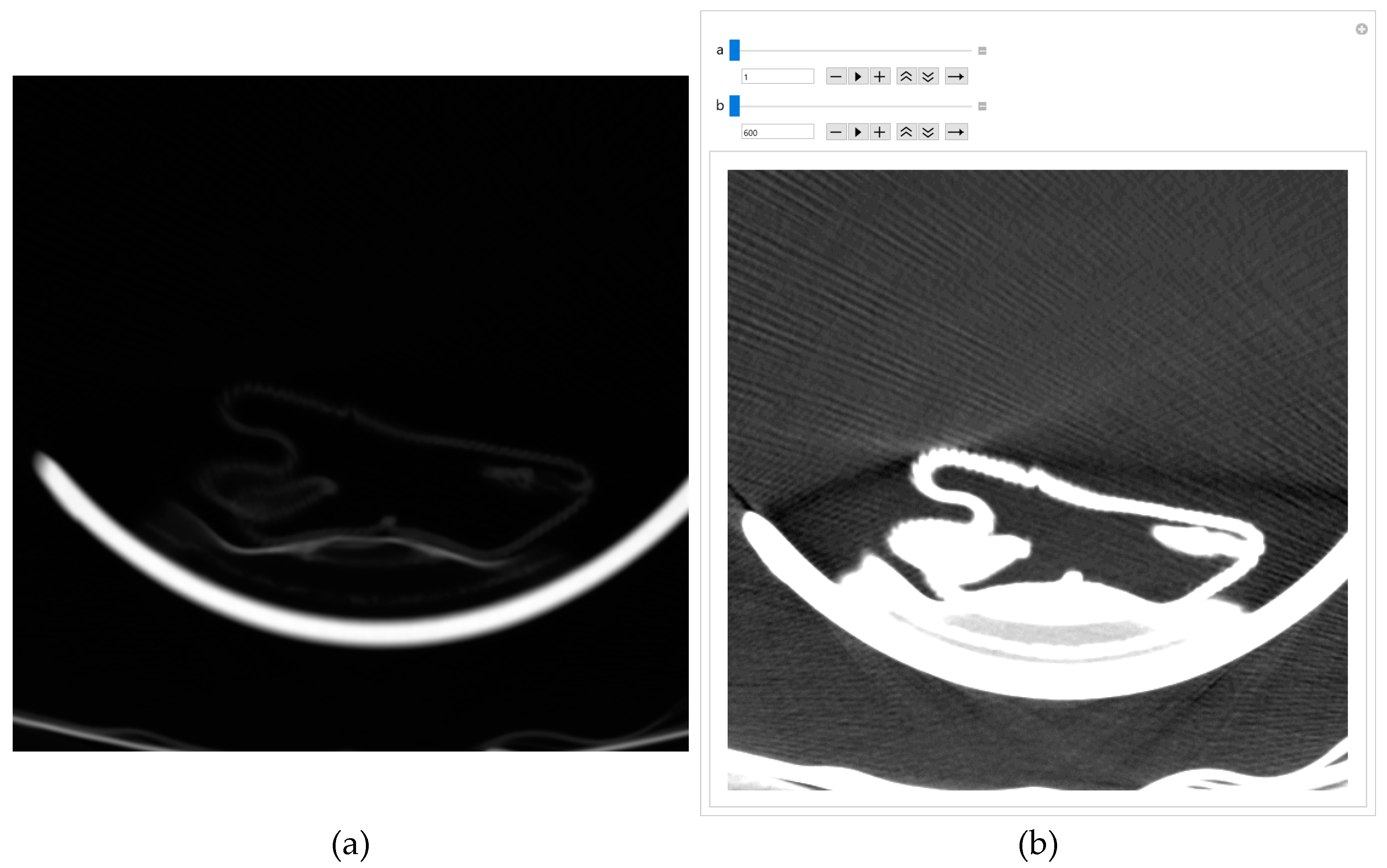
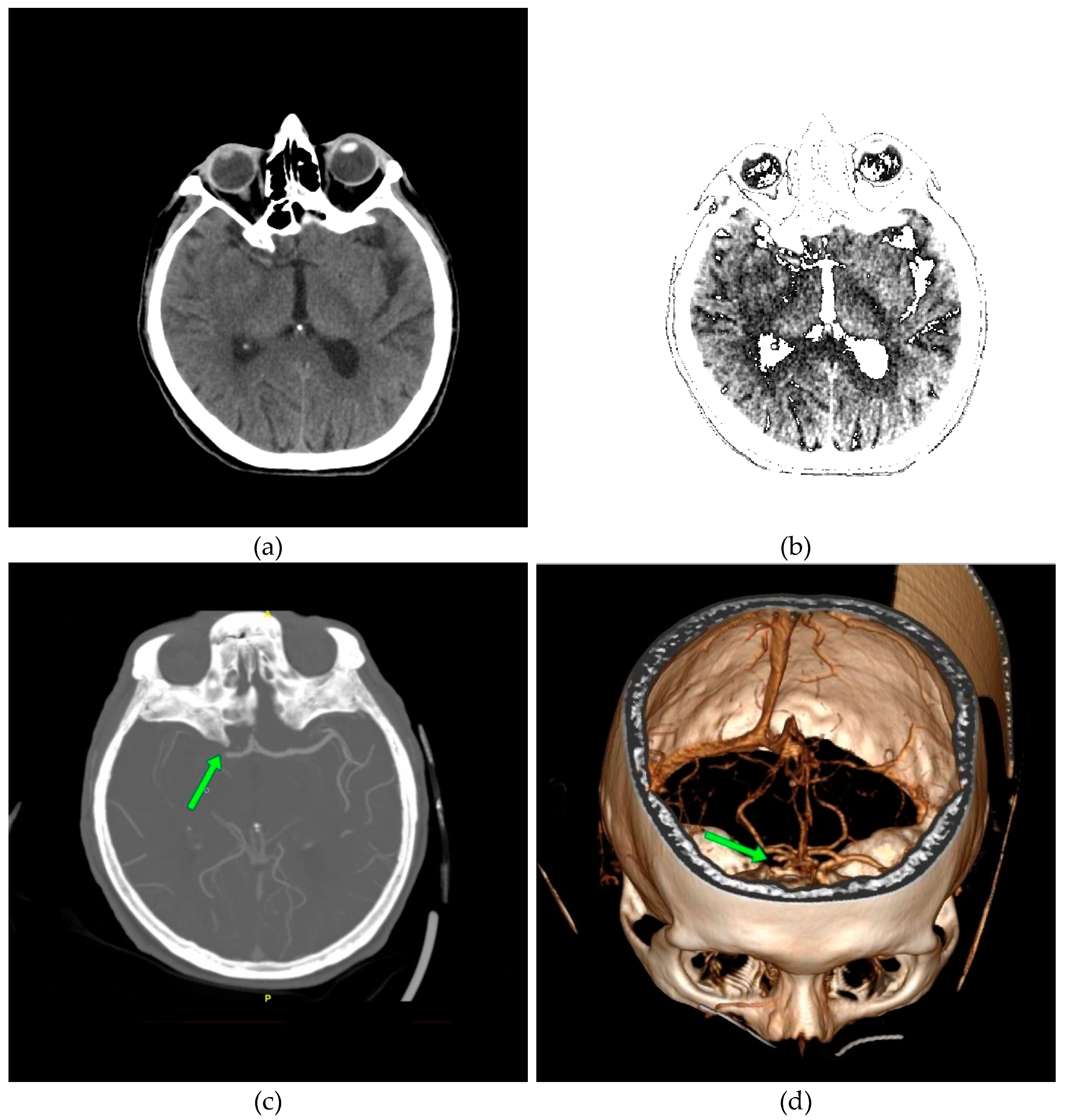
The original image's background and other unwanted artifacts (Figure 9a) can be removed by adjusting the minimum and maximum display pixel values using the sliders (shown in Figure A1b in Appendix A). Darker areas (values less than the one defined by the first slider) are displayed in white, especially on the ethmoidal air cells. Bone values and all other values obtained by another slider are also displayed in white. All other gray values are displayed in the maximum raster from 0 to 1, thus increasing the contrast, as shown in Figure 9b.
Images downloaded from the Internet after conversion from DCM format are often dark, and nothing can be seen on them. A few pixels with large values do not allow the valid pixels to be seen on a linear scale, i.e., the PNG image is almost entirely black. There are cases where, even with ImageAdjust, the image is completely dark again. Suppose the specialist suspects that a dark image still contains valuable information. In that case, he can use the same GUI to remove unwanted artifacts, as shown in Appendix A, where Figure A1a shows the original image, and Figure A1b shows the same image without artifacts, with GUI sliders for picture adjusting.
If the specialist concludes that the medical imaging does not contain valuable information, he immediately deletes it. About 3% of images downloaded from the Internet and converted to PNG format were deleted after the specialist ensured they did not contain useful information. Another way to conclude if the content of an image is valuable is to find how many different pixel values are in the image. If the image is black, and the number of different pixels is 1, it can be deleted because it has no applicable content.
One of the images in DCM format that the specialist singled out as potentially interesting by texture, after conversion to PNG format, with the ImageAdjust function, the central part of the image has been recognized (presented in Figure 9c). By eliminating artifacts using the proposed algorithm, Figure 9d is obtained, where the contrast in the central part is increased, brain parenchyma is more clearly visible, and the background, parts of the apparatus, and bones are shown in white.
Glimpse in Figure 9d, a more precise representation of the parenchyma is seen, as the brain sulci and gray-white mass border (Corticomedullary Border) can be observed, and possible bone artifacts can be reduced, which could contribute to an adequate visualization and interpretation of findings. The denoising effect [30,31,32,33] in this view in Figure 9d would significantly contribute to the image analysis.
2.7. Software Performance from Realistic and Actual Data
To evaluate the performance of the software, we used accurate and actual medical images of 26 patients in a total number of 2021 axial section images of the native MDCT examination. We reduced disk space usage by 66.9% by converting DCM format to PNG format. By converting the DICOM standard format into PNG format, we thoroughly ensured data privacy, both about the patient, the doctor, and the institution, while all other valuable values of the image remained unchanged and without losses. Any links to confidential and personal data have been deleted by deleting the original DICOM format. After there are images in PNG format, which have the same integer values as the authentic images in DICOM format, all further processing is done in PNG format.
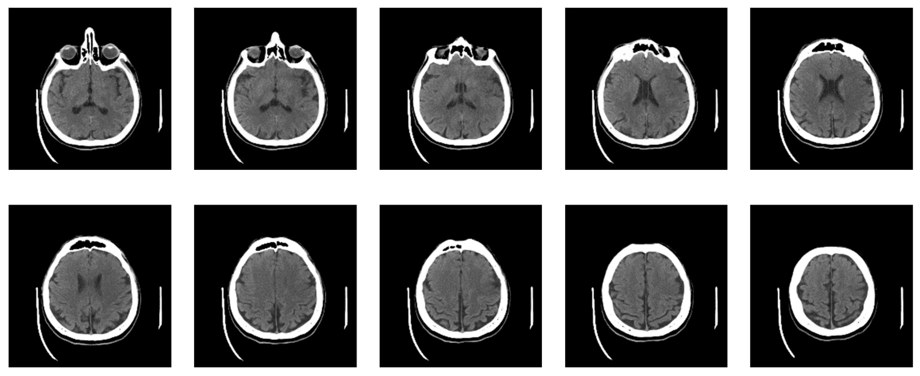
Now, the specialist has defined nine classes, five of which constitute actual neuroradiologically supported diagnoses of brain disease (Figure 10): (a) Glioblastoma Multiforme (GBM); (b) Metastases; (c) Pleomorphic Xanthoastrocytoma (PXA); (d) Hemorrhage; and (e) Stroke, i.e., Ischemia; while the other 4 are: (f) Normal; Bones; Empty and Irrelevant. Then, the classifier was applied based on labeled examples of a set of input/output pairs: imgEBTNSV = Classify[{imgB0[[1]] -> "Bones", imgE0[[2]] -> "Empty", imgG0[[3]] -> "GlioblastomaGBM", imgH0[[1]] -> "Stroke", imgI0[[2]] -> "Irrelevant", imgM0[[3]] -> "Metastases", imgN0[[1]] -> "Normal", imgP0[[2]] -> "PleomorphicPXA", imgR0[[3]] -> "Hemorrhage"...}];.
Figure 10 shows 6 of the nine defined classes. Bones, Empty and Irrelevant, are not shown in Figure 10 because they do not represent interest classes.
The classifier performed the following classification from the actual data set of 2021 images: 972 images (48.1%) into the Bones; 458 images (22.7%) into the Empty; into the Glioblastoma Multiforme – GBM 138 images (6.8%); into the Hemorrhage 13 images (0.6%); into the Irrelevant 326 images (16.1%); into the Metastases 45 images (2.2%); into the Normal 25 images (1.2%); into the Pleomorphic Xanthoastrocytoma – PXA 14 images (0.7%); and into the Stroke 30 images (1.5%).
A specialist performs further evaluation by selecting images for the Stroke class review using the random sample method. Out of 26 patients, as many as the data set contained, in two patients, the Stroke, i.e., Ischemia, was confirmed by MDCT angiography and MDCT perfusion. The classifier sorted 30 images out of 2021 into the Stroke class, which is 1.5%. All 30 images, which the classifier sorted into the Stroke class, are axial cross-sections of the brain parenchyma of two patients with a confirmed diagnosis of Stroke. Analyzing such sorted images by a physician specialist, it was observed that the classifier classified the images into the Stroke class with 100% accuracy. This can be a guideline when choosing further diagnostic procedures. Classified images are shown in Appendix B.
The specialist selected images from the class Stroke for further analysis. A characteristic image of the axial section of the original image is shown in Figure 11a. To compare and visualize the display of the original image, the specialist opens it in the presented GUI (Figure 11b) by selecting the parameters of the GUI options with 24 successive pixels, which gives the most precise visual representation to the physician specialists for analysis. The specialist noticed a darker part on the left side, indicating a brain change. After suspecting the existence of a Stroke, he makes further comparisons with further diagnostic methods, MDCT perfusion (Figure 11c) and MDCT angiography (Figure 11d).
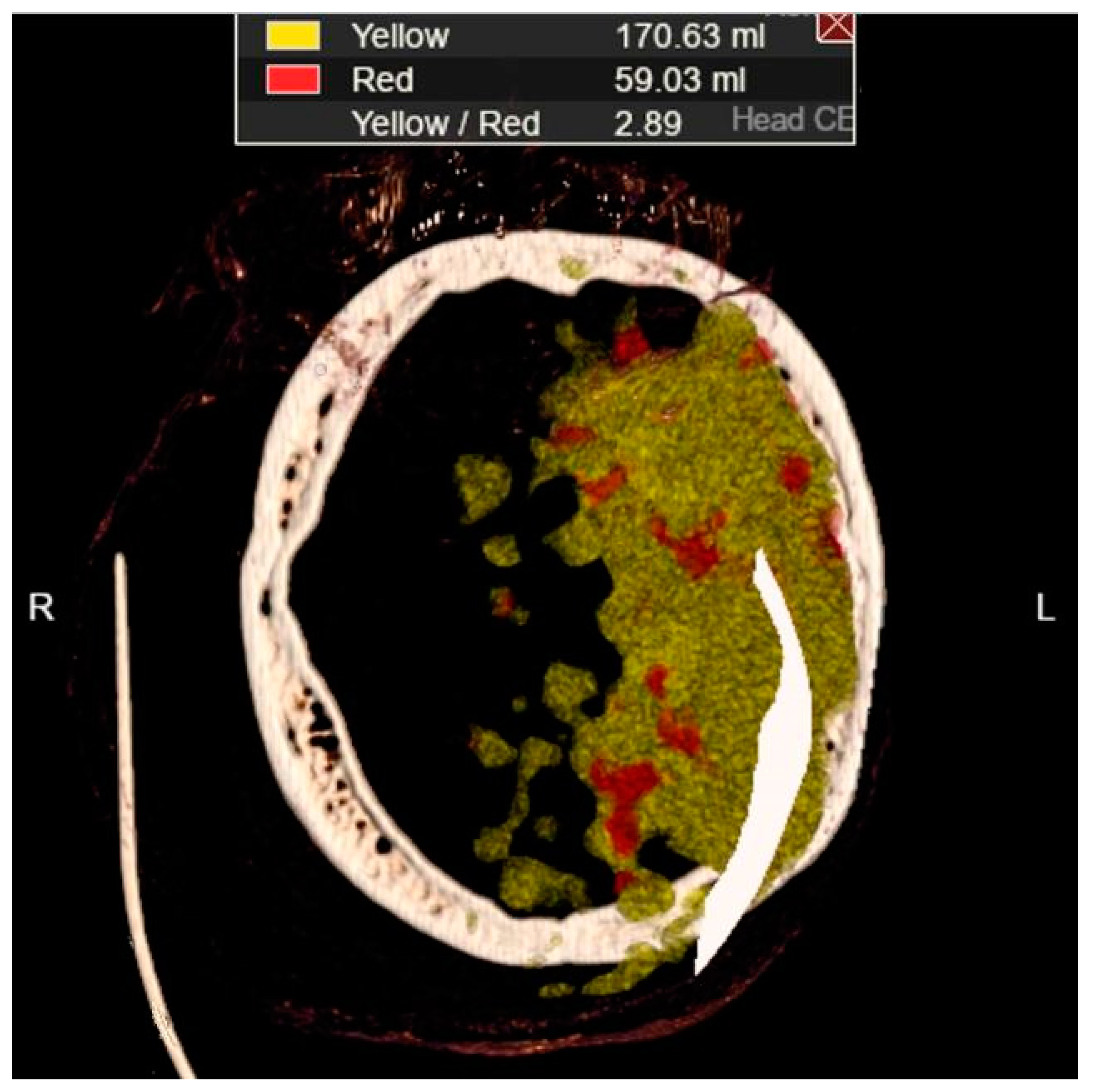
In Figure 11a, a discrete zone of hypodensity is seen in the left insular region on the native MDCT scan, which indicates acute ischemia more clearly visualized with GUI representation (Figure 11b). Figure 11c represents MDCT perfusion with a small red zone of the core and a larger yellow zone of the penumbra, and Figure 11d shows the occlusion of the left MCA (middle cerebral artery). Diagnosing acute ischemic lesions is challenging on native MDCT scans if cytotoxic edema and mass effect development have not yet occurred. The therapy of acute ischemia depends on the time that has passed since the onset of symptoms and the findings on MDCT imaging (changes in the brain parenchyma, defects in the post-contrast image of blood vessels, and the Core/Penumbra ratio (shown in the Figure A3 in Appendix C). It can be thrombolysis or thrombectomy. The core represents damaged tissue, and penumbra tissue is at risk of damage that can be salvageable. A better post-therapy outcome is expected in patients with smaller core and larger penumbra. Therefore, it is essential to apply adequate therapy promptly because it can save the tissue at risk of damage and affect the patient's mortality, morbidity, and quality of life. Visualization of acute brain ischemia on a native MDCT scan (Figure 11a) depends on the time of the examination concerning the onset of symptoms and the radiologist's experience. Here, the GUI (Figure 11b) can help in better and clearer visualization, and thus the interpretation of the findings and provide guidelines for the following diagnostic procedures and appropriate therapy.
In Figure 12a, a discrete zone of hypodensity is seen in the right basal ganglia region on the native MDCT scan, which indicates acute ischemia more clearly visualized with GUI representation (Figure 12b). Figure 12c,d show the occlusion of the right MCA (middle cerebral artery).
The scientific contribution of the work as the sum of all the previous is in the original method that enables reliable support for the diagnosis by specialists. This is the most significant contribution as the sum of all software contributions.
3. Discussion
A GUI was used for sorting purposes, where in 2 minutes, a physician specialist can sort about 100 images. Some images downloaded from the Internet contained pixels as rational numbers. The analysis was done by converting the pixel values, from 0 to 1, to integers to use the symbolic analysis in the Wolfram Language [29]. For the software to work correctly, it was first determined whether the adjacent values were around 1. If they were not, normalization was performed to use the minimum integer number of adjacent pixel values. Before the histogram analysis, the minimum and maximum values are determined so that the processing is performed with whole numbers that do not have large values, which is essential for the fast processing of a large number of medical imaging. Powerful, symbolic deep-learning frameworks and specialized pipelines for various data types, such as images, complement the proposed algorithm.
The hardware solution provides cost-efficient benefits, as all codes can be executed on the Rpi4 [34], for which all software is free. All medical imaging is on the SD memory card, operating system, and application software. After the analysis, the specialist can remove the memory card and keep it with him or execute it on other hardware in another place. This way, all data is protected, and no one can access the data on the card nor have an insight into the specialist's analysis and conclusions. Each specialist can create his database of medical imaging. Modified images without private data, the specialist can dis-tribute via mobile devices, expecting an unbiased assessment from colleagues worldwide.
During our research, we observed different image statistics, a product of different manufacturer scanner settings. A significant segment of the future upgrade of our projected analytical model would be reflected through an upgrade of the GUI in the form of an additional Toolbar menu that will allow specialists to easily select the scanner model on which the patient was examined. This way, we would ensure that our realized model can be applied to imaging devices from different manufacturers and independent medical institutions.
In actual application in clinical practice, the proposed method could significantly contribute to comparing new medical imaging with existing ones when dealing with rare diseases or diseases presented atypically. In this way, it would be possible to speed up not only the establishment of a differential diagnosis but also influence the selection of further diagnostic procedures and adequate and timely therapy. This would be of great importance for the outcome of the therapy and, thus, for improving the patient's health and quality of life.
At this stage, the software provides favorable support to the specialist's diagnosis so that at each subsequent examination, the specialist could use our proposed method of image classification and their distribution into predefined classes of existing diseases and monitor the program's execution. If the specialist, by reviewing the classification of the images after the program's execution, suspects the existence of changes in the patient's brain in a specific class, and additional diagnostics confirm this, those would be flawless results. During the time and further work on improving the software, our proposed model could help physicians in quick decision-making to apply further diagnostic methods and differential diagnosis for timely therapy and a more favorable outcome.
Author Contributions
Conceptualization, A.S. and S.L.; Data curation, S.L.; Investigation, S.L.; Methodology, A.S. and M.L.-B.; Project administration, S.L. and K.D.; Resources, S.L. and K.D.; Software, A.S. and M.L.-B.; Validation, S.L.; Formal Analysis, A.S. and M.L.-B.; Visualization, A.S. and M.L.-B.; Supervision, A.S.; Writing—original draft, A.S.; Writing—review & editing, A.S., M.L.-B., S.L., and K.D.; Funding Acquisition, K.D. All authors have read and agreed to the published version of the manuscript.
Funding
This research received no external funding.
Institutional Review Board Statement
Not applicable.
Informed Consent Statement
Not applicable. Images presented in the paper have no confidential personal data of patients, and individual rights are not infringed, as is detailed in the manuscript. Personal identity details on brain images (names, dates of birth, and identity numbers) are secured and completely anonymous. The information is anonymized, and the submission does not include images that may identify the person.
Data Availability Statement
The data presented in this study are available from the corresponding author upon reasonable request.
Acknowledgments
Not applicable.
Conflicts of Interest
The authors declare no conflict of interest.
Appendix A
Figure A1.
Picture adjusting with GUI: (a) the original image; (b) the same image without artifacts, with GUI sliders for picture adjusting.
Figure A1.
Picture adjusting with GUI: (a) the original image; (b) the same image without artifacts, with GUI sliders for picture adjusting.
Appendix B
Figure A2.
The result: The classifier sorted 30 images out of 2021 from 26 patients with confirmed diseases into the Stroke class with 100% accuracy.
Figure A2.
The result: The classifier sorted 30 images out of 2021 from 26 patients with confirmed diseases into the Stroke class with 100% accuracy.
Appendix C
Figure A3.
Core/Penumbra ratio: The core represents damaged tissue, and penumbra tissue is at risk of damage that can be salvageable.
Figure A3.
Core/Penumbra ratio: The core represents damaged tissue, and penumbra tissue is at risk of damage that can be salvageable.
References
- Simović, A.; Lutovac-Banduka, M.; Lekić, S.; Kuleto, V. Smart Visualization of Medical Images as a Tool in the Function of Education in Neuroradiology. Diagnostics 2022, 12, 3208. [Google Scholar] [CrossRef] [PubMed]
- Myszczynska, M.A.; Ojamies, P.N.; Lacoste, A.M.; Neil, D.; Saffari, A.; Mead, R.; Hautbergue, G.M.; Holbrook, J.D.; Ferraiuolo, L. Applications of machine learning to diagnosis and treatment of neurodegenerative diseases. Nature Reviews Neurology 2020, 16, 440–456. [Google Scholar] [CrossRef] [PubMed]
- Najjar, R. Redefining Radiology: A Review of Artificial Intelligence Integration in Medical Imaging. Diagnostics 2023, 13, 2760. [Google Scholar] [CrossRef] [PubMed]
- Kim, D.; Lee, J.H.; Kim, S.W.; Hong, J.M.; Kim, S.J.; Song, M.; Choi, J.M.; Lee, S.Y.; Yoon, H.; Yoo, J.Y. Quantitative measurement of pneumothorax using artificial intelligence management model and clinical application. Diagnostics 2022, 12, 1823. [Google Scholar] [CrossRef]
- Balasubramanian, P. K.; Lai, W. C.; Seng, G. H.; Selvaraj, J. Apestnet with mask r-cnn for liver tumor segmentation and classification. Cancers 2023, 15, 330. [Google Scholar] [CrossRef] [PubMed]
- Sousa, J.; Pereira, T.; Silva, F.; Silva, M. C.; Vilares, A. T.; Cunha, A.; Oliveira, H. P. Lung Segmentation in CT Images: A Residual U-Net Approach on a Cross-Cohort Dataset. Applied Sciences 2022, 12, 1959. [Google Scholar] [CrossRef]
- Primakov, S.P.; Ibrahim, A.; van Timmeren, J.E.; Wu, G.; Keek, S.A.; Beuque, M.; Granzier, R.W.; Lavrova, E.; Scrivener, M.; Sanduleanu, S.; Kayan, E; et. al. Automated detection and segmentation of non-small cell lung cancer computed tomography images. Nature communications 2022, 13, 3423. [Google Scholar] [CrossRef]
- Li, K.; Yu, L.; Heng, P. A. Towards reliable cardiac image segmentation: Assessing image-level and pixel-level segmentation quality via self-reflective references. Medical Image Analysis 2022, 78, 102426. [Google Scholar] [CrossRef]
- Li, R.; Xiao, C.; Huang, Y.; Hassan, H.; Huang, B. Deep learning applications in computed tomography images for pulmonary nodule detection and diagnosis: A review. Diagnostics 2022, 12, 298. [Google Scholar] [CrossRef]
- Ruffle, J. K.; Mohinta, S.; Gray, R.; Hyare, H.; Nachev, P. Brain tumour segmentation with incomplete imaging data. Brain Communications 2023, 5, fcad118. [Google Scholar] [CrossRef]
- Ghaffari, M.; Samarasinghe, G.; Jameson, M.; Aly, F.; Holloway, L.; Chlap, P.; Koh, E.S.; Sowmya, A.; Oliver, R. Automated post-operative brain tumour segmentation: A deep learning model based on transfer learning from pre-operative images. Magnetic resonance imaging 2022, 86, 28–36. [Google Scholar] [CrossRef] [PubMed]
- Gaur, L.; Bhandari, M.; Razdan, T.; Mallik, S.; Zhao, Z. Explanation-driven deep learning model for prediction of brain tumour status using MRI image data. Frontiers in genetics 2022, 13, 448. [Google Scholar] [CrossRef] [PubMed]
- Zheng, Y.; Wang, S.; Li, Q.; Li, B. Fringe projection profilometry by conducting deep learning from its digital twin. Optics Express 2020, 28, 36568–36583. [Google Scholar] [CrossRef] [PubMed]
- Jiang, Y.; Zhao, K.; Xia, K.; Xue, J.; Zhou, L.; Ding, Y.; Qian, P. A novel distributed multitask fuzzy clustering algorithm for automatic MR brain image segmentation. Journal of medical systems 2019, 43, 1–9. [Google Scholar] [CrossRef]
- Long, J.; Shelhamer, E.; Darrell, T. Fully convolutional networks for semantic segmentation. In Proceedings of the IEEE conference on computer vision and pattern recognition 2015, 3431–3440. [Google Scholar]
- Hu, M.; Zhong, Y.; Xie, S.; Lv, H.; Lv, Z. Fuzzy system based medical image processing for brain disease prediction. Frontiers in Neuroscience 2021, 15, 714318. [Google Scholar] [CrossRef]
- Xie, Y.; Zaccagna, F.; Rundo, L.; Testa, C.; Agati, R.; Lodi, R.; Manners, D.N.; Tonon, C. Convolutional neural network techniques for brain tumor classification (from 2015 to 2022): Review, challenges, and future perspectives. Diagnostics 2022, 12, 1850. [Google Scholar] [CrossRef] [PubMed]
- Salehi, A.W.; Khan, S.; Gupta, G.; Alabduallah, B.I.; Almjally, A.; Alsolai, H.; Siddiqui, T.; Mellit, A. A Study of CNN and Transfer Learning in Medical Imaging: Advantages, Challenges, Future Scope. Sustainability 2023, 15, 5930. [Google Scholar] [CrossRef]
- Mun, S. K.; Wong, K. H.; Lo, S. C. B.; Li, Y.; Bayarsaikhan, S. Artificial intelligence for the future radiology diagnostic service. Frontiers in molecular biosciences 2021, 7, 614258. [Google Scholar] [CrossRef]
- Esterhuizen, J. A.; Goldsmith, B. R.; Linic, S. Interpretable machine learning for knowledge generation in heterogeneous catalysis. Nature Catalysis 2022, 5, 175–184. [Google Scholar] [CrossRef]
- Shao, W.; Zhou, B. Effect of Coupling Medium on Penetration Depth in Microwave Medical Imaging. Diagnostics 2022, 12, 2906. [Google Scholar] [CrossRef]
- Kaggle. Available online: https://www.kaggle.com/competitions/rsna-intracranial-hemorrhage-detection (accessed on March 10, 2021).
- Beuter, C.; Oleskovicz, M. S-transform: from main concepts to some power quality applications. IET Signal Processing 2020, 14, 115–123. [Google Scholar] [CrossRef]
- Mukhamediev, R.I.; Popova, Y.; Kuchin, Y.; Zaitseva, E.; Kalimoldayev, A.; Symagulov, A.; Levashenko, V.; Abdoldina, F.; Gopejenko, V.; Yakunin, K.; Muhamedijeva, E.; et al. Review of Artificial Intelligence and Machine Learning Technologies: Classification, Restrictions, Opportunities and Challenges. Mathematics 2022, 10, 2552. [Google Scholar] [CrossRef]
- Goodfellow, I.; Bengio, Y.; Courville, A. Deep learning. MIT press, Cambridge, Massachusetts, London, England, 2016; 1-768.
- Oyewole, G.J.; Thopil, G.A. Data clustering: Application and trends. Artificial Intelligence Review 2023, 56, 6439–6475. [Google Scholar] [CrossRef] [PubMed]
- Forootan, M.M.; Larki, I.; Zahedi, R.; Ahmadi, A. Machine learning and deep learning in energy systems: A review. Sustainability 2022, 14, 4832. [Google Scholar] [CrossRef]
- Lutovac-Banduka, M.; Simović, A.; Orlić, V.; Stevanović, A. Dissipation Minimization of Two-stage Amplifier using Deep Learning. SJEE 2023, 20, 129–145. [Google Scholar] [CrossRef]
- Bernard, E. Introduction to Machine Learning. Wolfram Media inc., December 20, 2021, USA, 1-424.
- Sagheer, S.V.M.; George, S.N. A review on medical image denoising algorithms. Biomedical signal processing and control 2020, 61, 102036. [Google Scholar] [CrossRef]
- Diwakar, M.; Kumar, M. A review on CT image noise and its denoising. Biomedical Signal Processing and Control 2018, 42, 73–88. [Google Scholar] [CrossRef]
- Zhang, Y.; Xu, S.; Li, H.; Kong, Z.; Xiang, X.; Cheng, X.; Liu, S. Deep learning-based denoising in brain tumor cho pet: Comparison with traditional approaches. Applied Sciences 2022, 12, 5187. [Google Scholar] [CrossRef]
- Kim, I.; Kang, H.; Yoon, H.J.; Chung, B.M.; Shin, N.Y. Deep learning–based image reconstruction for brain CT: improved image quality compared with adaptive statistical iterative reconstruction-Veo (ASIR-V). Neuroradiology 2021, 63, 905–912. [Google Scholar] [CrossRef]
- Raspberry Pi 4. Available online: https://www.raspberrypi.com/products/raspberry-pi-4-model-b/ (accessed on September 10, 2023).
Figure 1.
Examples of images of characteristic classes: (a) Nothing; (b) Something; (c) Empty; (d) Bones; and (e) Visible.
Figure 1.
Examples of images of characteristic classes: (a) Nothing; (b) Something; (c) Empty; (d) Bones; and (e) Visible.
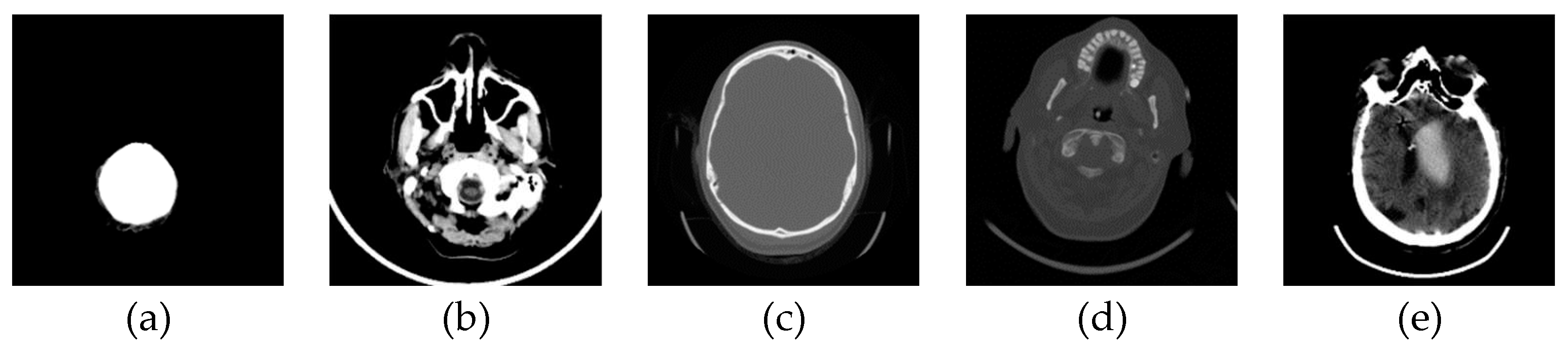
Figure 2.
Selected representatives of the classes in lists where is: v={visible}; b={bones}; s={something}; e={empty}; and n={nothing}.
Figure 2.
Selected representatives of the classes in lists where is: v={visible}; b={bones}; s={something}; e={empty}; and n={nothing}.
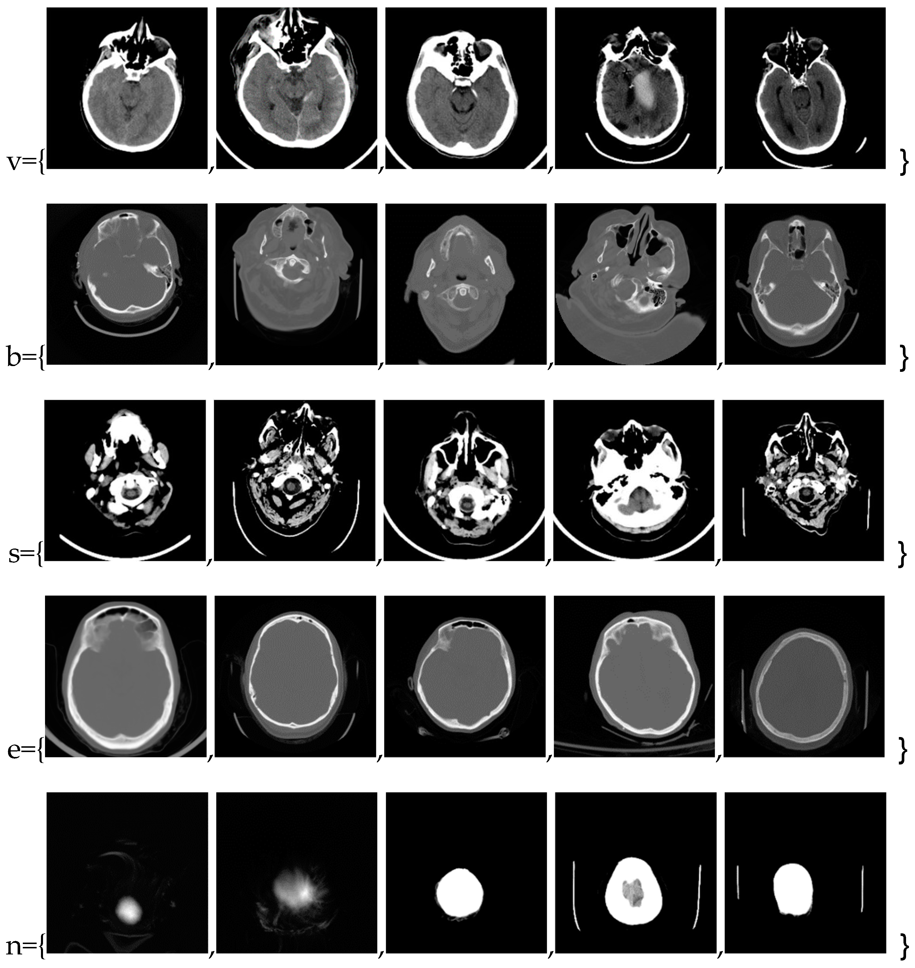
Figure 3.
The S transform representation.
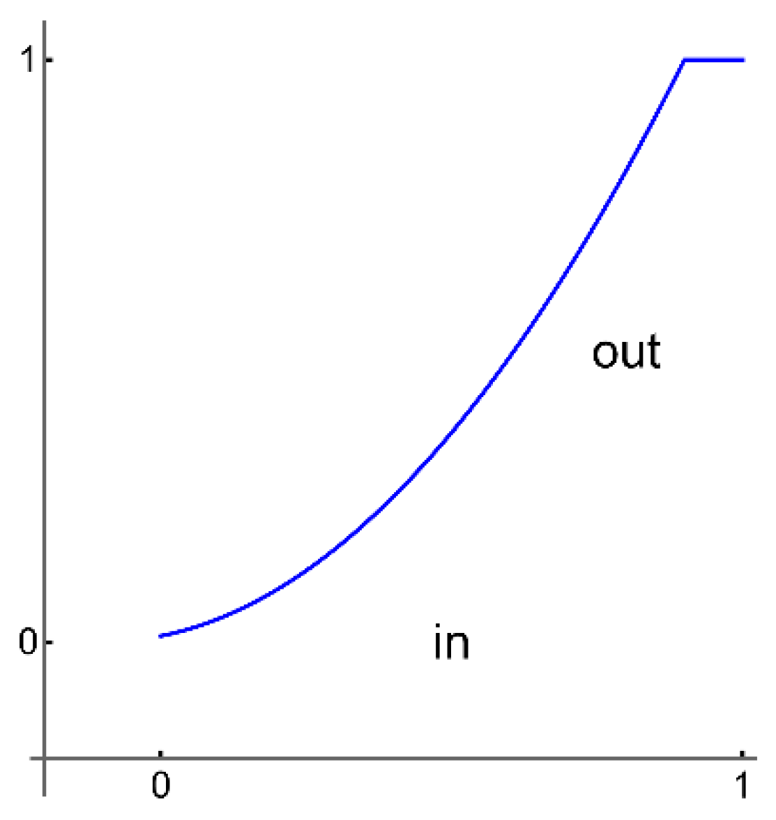
Figure 4.
Graphical, User-friendly Interface (GUI): (a) selected image for classification; (b) display image name and class selection drop-down list; and (c) selection of the class to which the selected image belongs.
Figure 4.
Graphical, User-friendly Interface (GUI): (a) selected image for classification; (b) display image name and class selection drop-down list; and (c) selection of the class to which the selected image belongs.
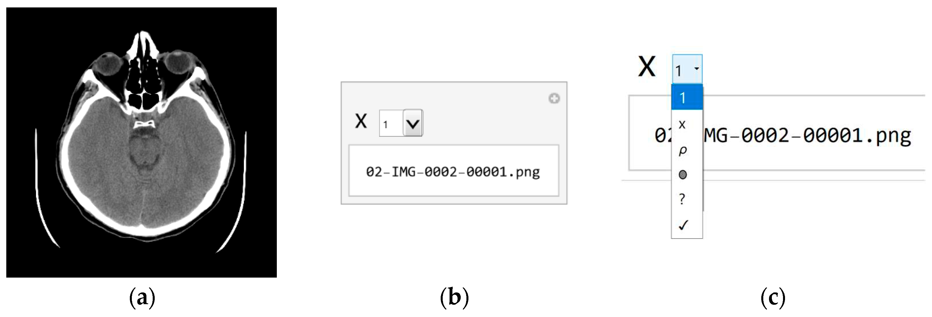
Figure 5.
The results: 14 images out of 397,994.
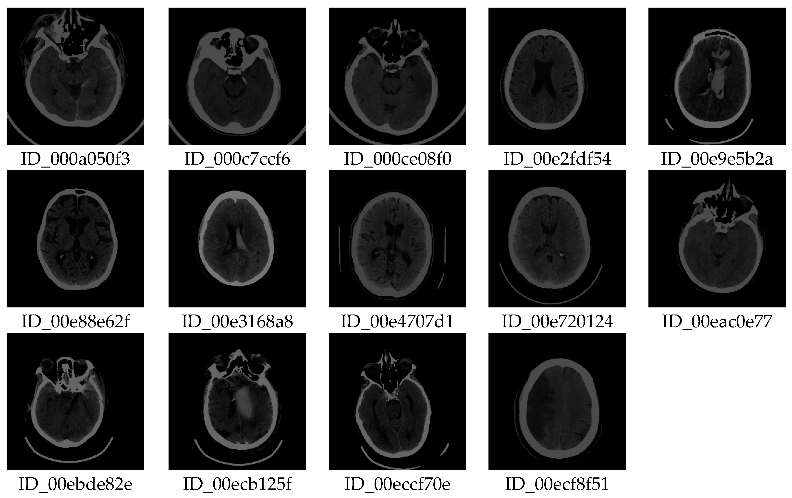
Figure 6.
Histogram of the image with pixels values: (a) range of valuable pixels from 1 to 100; and (b) averaged histogram of 24 consecutive pixels.
Figure 6.
Histogram of the image with pixels values: (a) range of valuable pixels from 1 to 100; and (b) averaged histogram of 24 consecutive pixels.
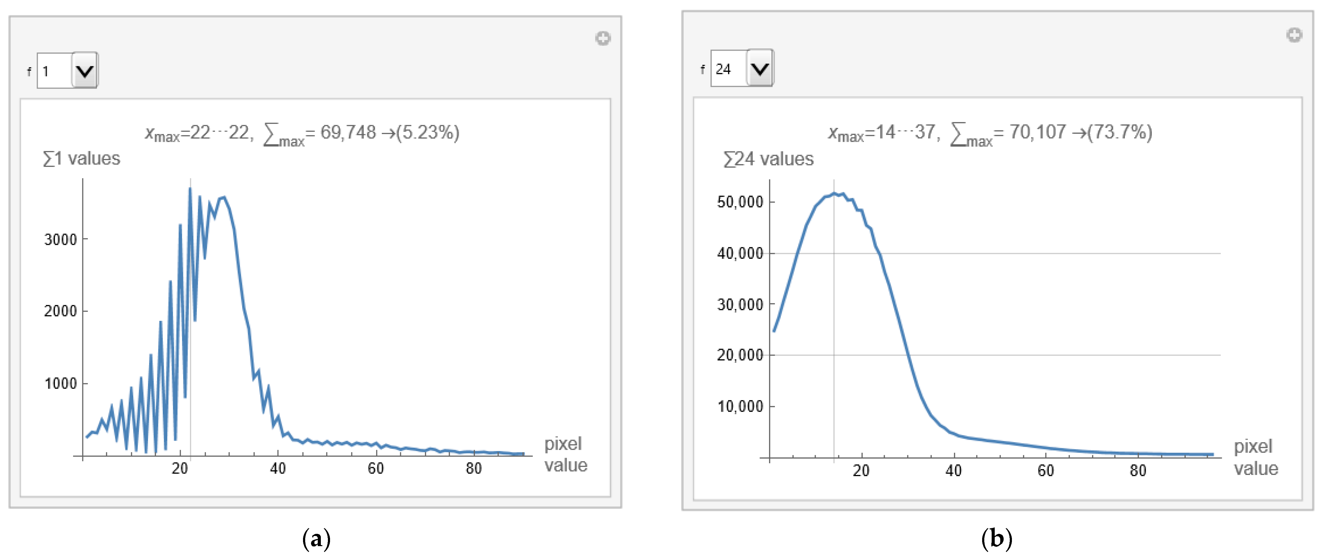
Figure 7.
GUI displays: (a) 99 consecutive pixels; (b) 65 consecutive pixels; and (c) 48 consecutive pixels.
Figure 7.
GUI displays: (a) 99 consecutive pixels; (b) 65 consecutive pixels; and (c) 48 consecutive pixels.
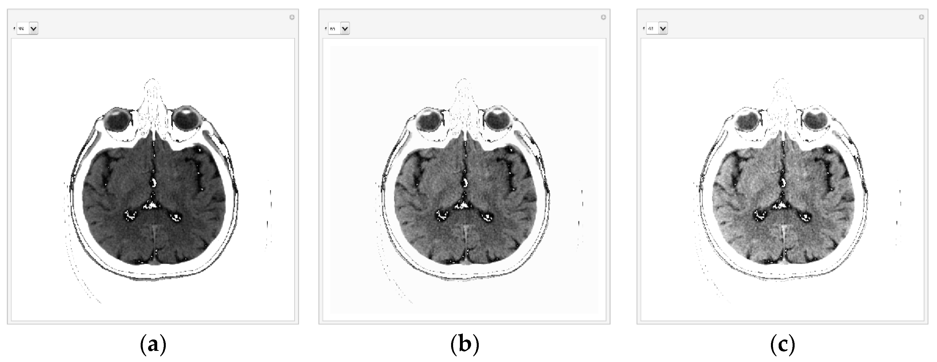
Figure 8.
Histograms for medical images that have different pixel value statistics: (a) valuable pixels in the value range of ≈ 1000; (b) pixel value in the range from 850 to 1200.
Figure 8.
Histograms for medical images that have different pixel value statistics: (a) valuable pixels in the value range of ≈ 1000; (b) pixel value in the range from 850 to 1200.
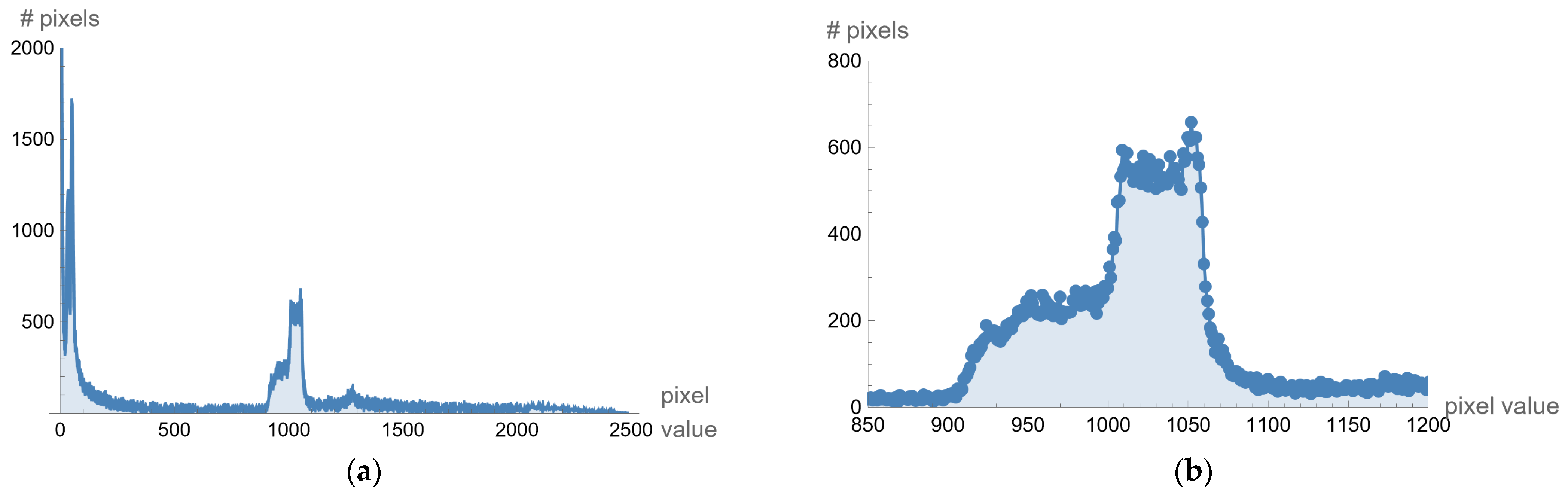
Figure 9.
Adjusting the minimum and maximum pixel values: (a) the original image; (b) displayed in the maximum raster from 0 to 1, thus increasing the contrast; (c) ImageAdjust function to image recognition; (d) artifact elimination so as the brain parenchyma is clearly visible.
Figure 9.
Adjusting the minimum and maximum pixel values: (a) the original image; (b) displayed in the maximum raster from 0 to 1, thus increasing the contrast; (c) ImageAdjust function to image recognition; (d) artifact elimination so as the brain parenchyma is clearly visible.
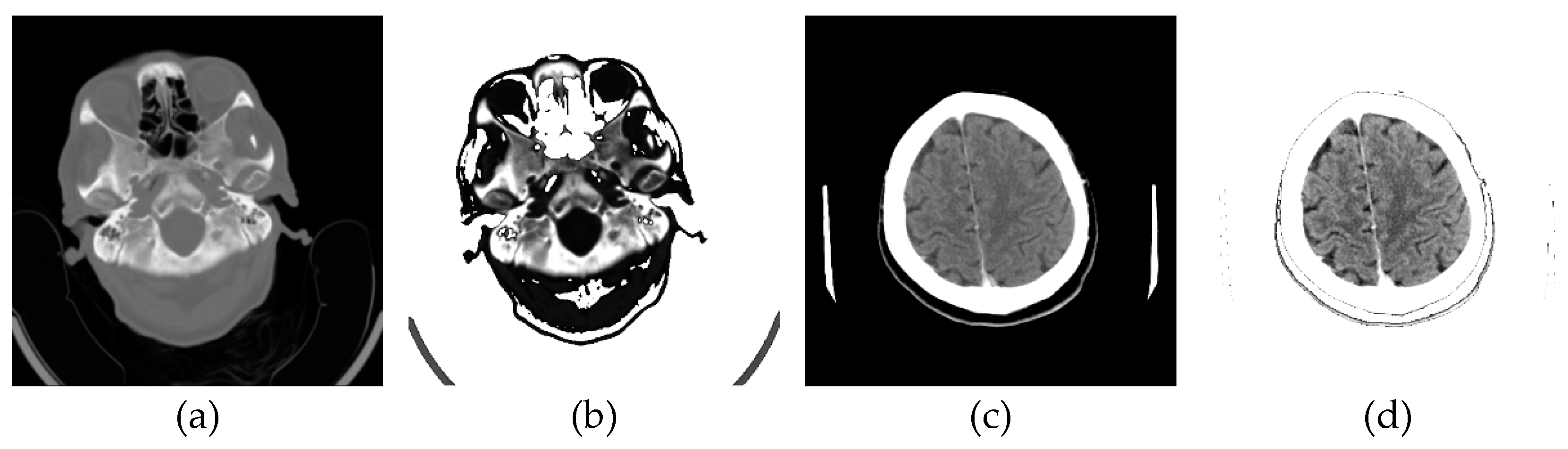
Figure 10.
Relevant samples of confirmed diseases and the Normal brain sample: a) Glioblastoma Multiforme (GBM); (b) Metastases; (c) Pleomorphic Xanthoastrocytoma (PXA); (d) Hemorrhage (e) Stroke; and (f) Normal.
Figure 10.
Relevant samples of confirmed diseases and the Normal brain sample: a) Glioblastoma Multiforme (GBM); (b) Metastases; (c) Pleomorphic Xanthoastrocytoma (PXA); (d) Hemorrhage (e) Stroke; and (f) Normal.
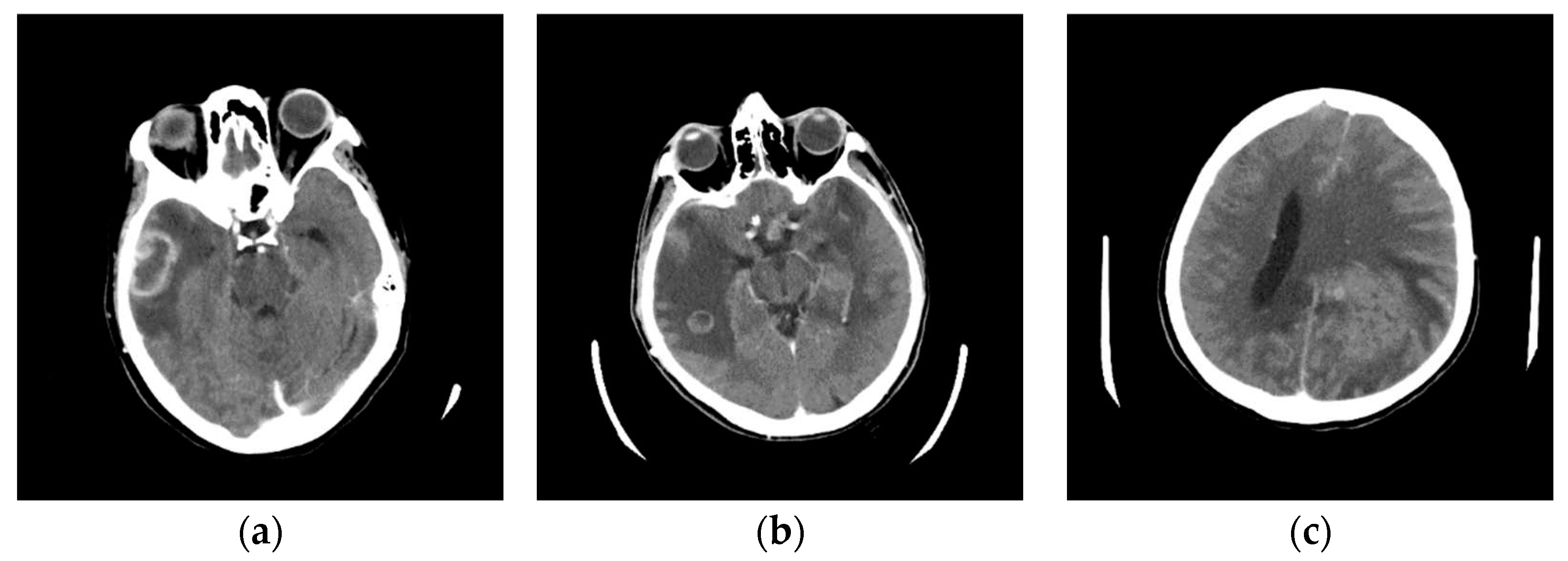
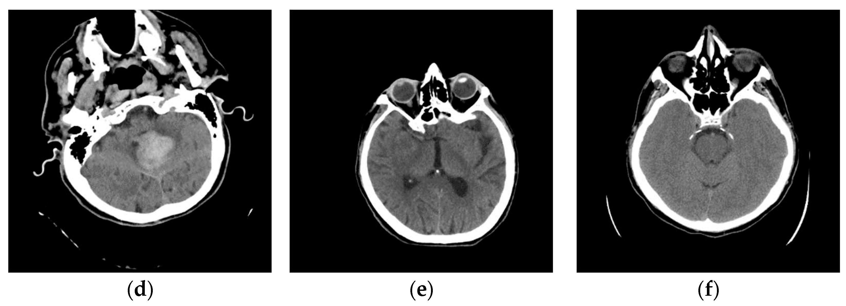
Figure 11.
Comparative presentation of the results of patient 1 with a confirmed diagnosis of Stroke: (a) Original image obtained from the MDCT scanner; (b) Image display of the same axial cress-section using the developed GUI with 24 successive pixels selected for display; (c) MDCT perfusion; (d) MDCT angiography – volume rendering (VR).
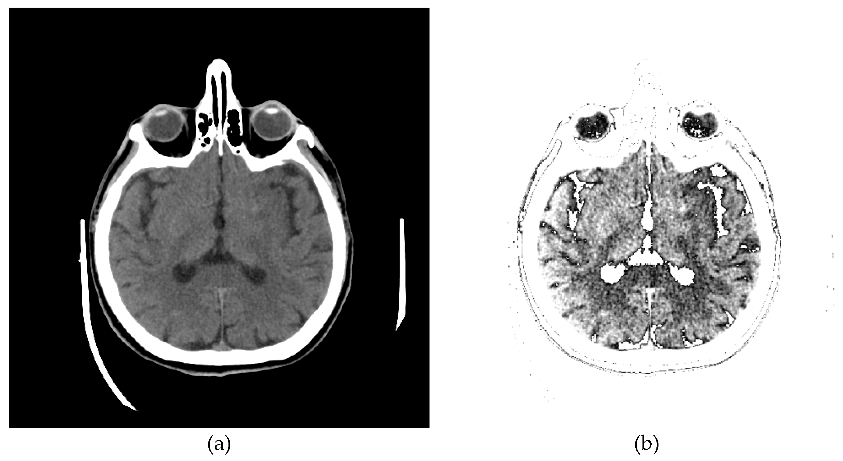
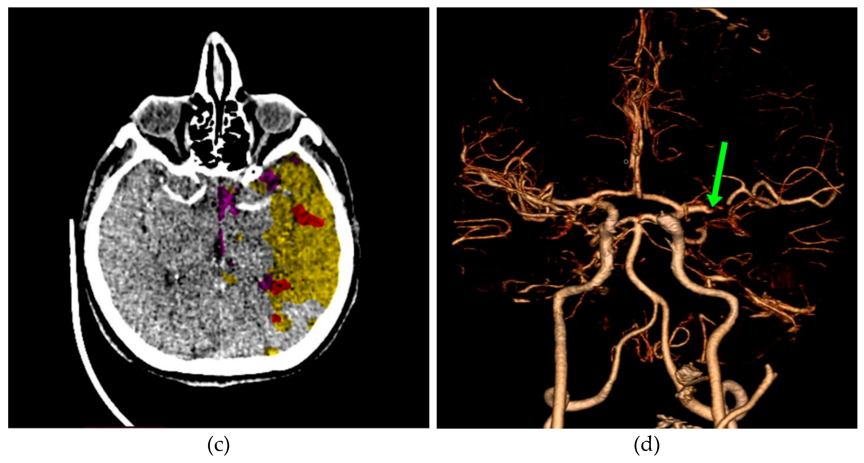
Figure 12.
Comparative presentation of the results of patient 2 with a confirmed diagnosis of Stroke: (a) Original image obtained from the MDCT scanner; (b) Image display of the same axial cress-section using the developed GUI with 24 successive pixels selected for display; (c) MDCT angiography – maximum intensity projection (MIP); (d) MDCT angiography – volume rendering (VR).
Disclaimer/Publisher’s Note: The statements, opinions and data contained in all publications are solely those of the individual author(s) and contributor(s) and not of MDPI and/or the editor(s). MDPI and/or the editor(s) disclaim responsibility for any injury to people or property resulting from any ideas, methods, instructions or products referred to in the content. |
© 2023 by the authors. Licensee MDPI, Basel, Switzerland. This article is an open access article distributed under the terms and conditions of the Creative Commons Attribution (CC BY) license (http://creativecommons.org/licenses/by/4.0/).
Copyright: This open access article is published under a Creative Commons CC BY 4.0 license, which permit the free download, distribution, and reuse, provided that the author and preprint are cited in any reuse.
supplementary.zip (2.15MB )
Submitted:
16 November 2023
Posted:
17 November 2023
You are already at the latest version
Alerts
supplementary.zip (2.15MB )
This version is not peer-reviewed
Submitted:
16 November 2023
Posted:
17 November 2023
You are already at the latest version
Alerts
Abstract
During a multi-detector computed tomography (MDCT) examination, it is crucial to efficiently organize, store, and transmit medical images in DICOM standard, which requires significant hardware resources and memory. Our project processed large amounts of DICOM images by classifying them based on cross-section views that may carry important information about a possible diagnosis. We ensured that images were retained and saved in PNG format to optimize hardware resources while preserving patient confidentiality. Furthermore, we have developed a graphical, user-friendly interface that allows physicians to visualize specific regions of interest in a patient's brain where changes may indicate disease. Our proposed method enables quick classification of medical images into predefined classes of confirmed diseases of brain parenchyma, contributing to swift decision-making for further diagnosis for more precisely evaluating and characterizing brain changes, and it can lead to the rapid application of adequate therapy, which may result in better outcomes.
Keywords:
Subject: Computer Science and Mathematics - Artificial Intelligence and Machine Learning
1. Introduction
In the scientific literature, many models have been proposed for detecting various brain diseases in patients. The Smart Visualization of Medical Images (SVMI) method [1], proposed in 2022, enables innovative visualization of medical images as a tool in the function of education in neuroradiology relevant to medical imaging research and provides a valuable tool for analyzing medical images.
Detecting brain diseases is a critical task that can be made easier and more accurate using artificial intelligence (AI) and machine learning (ML). By analyzing large amounts of data, ML algorithms can identify patterns and anomalies that may be difficult for humans to detect. This can lead to earlier and more accurate diagnoses and better patient outcomes. Myszczynska et al. [2] discuss how machine learning as a subfield of artificial intelligence can aid early diagnosis and interpretation of medical images and the discovery and development of new therapies. Najjar [3] shed light on AI applications in radiology, elucidating their seminal roles in image segmentation, computer-aided diagnosis, predictive analytics, and workflow optimization while fostering robust collaborations between specialists in the field of radiology and AI developers.
Segmentation and classification of medical images represent essential techniques for detecting various brain diseases and critical decision-making processes for the timely application of the right therapy. Precise segmentation of medical images of the brain brings valuable information to physicians for disease diagnosis, application of adequate therapy, and further pharmacological or surgical procedures. As a critical task, segmentation and classification of medical images involves separating an image into multiple regions, or segments, based on its features and characteristics and then classifying those segments into different categories. This process is used in various medical applications, such as disease diagnosis, treatment planning, and medical research. In the scientific and research literature, image segmentation and classification tasks include various approaches for disease detection on most organs in the human body. Kim et al. [4] have developed an AI model for estimating the amount of pneumothorax on chest radiographs using U-net that performed semantic segmentation and classification of pneumothorax and areas without pneumothorax. Balasubramanian et al. [5] apply a novel model for segmenting and classifying liver tumors built on an enhanced mask region-based convolutional neural network (R-CNN mask) used to separate the liver from the computed tomography (CT) abdominal image, with prevention of overfitting, the segmented picture is fed onto an enhanced swin transformer network with adversarial propagation (APESTNet). Sousa et al. [6] investigated the development of a deep learning (DL) model, whose architecture consists of the combination of two structures, a U-Net and a ResNet34. Primakov et al. [7] present a fully automated pipeline for the detection and volumetric segmentation of non-small cell lung cancer validated on 1328 thoracic CT scans from 8 institutions. Li Kang et al. [8] propose a reference-based framework to assess the image-level quality for overall evaluation and pixel-level quality to locate mis-segmented regions. In their work, Li Kang et al. proposed a reference-based framework to conduct thorough quality assessments on cardiac image segmentation results for reliable computer-aided cardiovascular disease diagnosis. Li Rui et al. [9] gave a review that focuses on segmentation and classification parts based on lung nodule type, general neural network and multi-view convolutional neural network architecture. Ruffle et al. [10] present brain tumor segmentation with incomplete imaging data based on magnetic resonance imaging (MRI) of 1251 individuals, where they quantify the comparative fidelity of automated segmentation models drawn from MR data, replicating the various levels of completeness observed in real life. Ghaffari et al. [11] developed an automated method for segmenting brain tumors into their sub-regions using an MRI dataset, which consists of multimodal postoperative brain scans of 15 patients who were treated with postoperative radiation therapy, along with manual annotations of their tumor sub-regions. Gaur et al. [12] used an explanation-driven dual-input CNN model to find if a particular MRI image is subjected to a tumor or not and used a dual-input CNN approach to prevail over the classification challenge with images of inferior quality in terms of noise and metal artifacts by adding Gaussian noise.
The scientific works mentioned above are only a glimpse of insight into recent literature. Many of the mentioned works and scientific research, with the application of advanced machine learning algorithms, can obtain accurate and reliable results, leading to better patient outcomes and more effective treatments. In neuroradiology, in the analysis of medical images by physicians and specialists, certain obstacles make it difficult or impossible to visualize and interpret the findings adequately. Disturbances are reflected as artifacts that mimic pathology, degrade image quality, and can occur due to patient movement during imaging or previous surgical or interventional radiologist procedures. Difficulties in recognizing and segmenting medical images of patients' brains can also be reflected in other noises, such as the poor resolution of the device during setup or beam hardening caused by the presence of a metal element in the patient's body that makes it difficult for the device's beam to penetrate the patient. Zheng et al. [13] have emphasized the significance of accurately processing medical images affected by solid noise and geometric distortions, as it plays a crucial role in clinical diagnosis and treatment. The limitations of grayscale images, such as poor contrast and the complexity of medical images obtained from MDCT and MRI devices, with individual variability, make MR brain image segmentation a challenging task. Jiang et al. [14] proposed a distributed multitask fuzzy c-means clustering algorithm that shows promise in improving the accuracy of MR brain image segmentation. This algorithm extracts knowledge among different clustering tasks. It exploits the standard information among different but related brain MR image segmentation tasks, thus avoiding the adverse effects caused by noisy data existing in some MR images.
In recent years, there have been significant advancements in the field of machine learning for medical image processing. Application of deep learning techniques, such as convolutional neural networks (CNNs) and recurrent neural networks (RNNs), medical images can now be analyzed and interpreted with greater accuracy and efficiency. These advancements have the potential to revolutionize medical diagnosis and treatment, as they enable healthcare professionals to detect and diagnose diseases earlier and with higher precision. These advancements have enabled accurate classification of medical images obtained from various devices and apparatus. Long et al. [15] adapted contemporary classification networks into fully convolutional networks and transferred their learned representations to detailed segmentation of brain cancer. In their study, Hu Mandong et al. [16] introduced a model that utilizes improved fuzzy clustering to predict brain disease diagnosis and process medical images obtained from MRI devices. They incorporated several techniques, including CNN, RNN, Fuzzy C-Means (FCM), Local Density Clustering Fuzzy C-Means (LDCFCM), and Adaptive Fuzzy C-Means (AFCM), in simulation experiments to compare their performance. As convolutional neural networks are a widely used deep learning approach to the brain tumor diagnosis, Xie et al. [17] present a comprehensive review of studies using CNN architectures for the classification of brain tumors using MR images to identify valuable strategies and possible obstacles in this development. Salehi et al. [18] analyze the importance of CNN improvements in image analysis and classification tasks and review the advantages of CNN and transfer learning in medical imaging, including improved accuracy, reduced time and resource requirements, and the ability to resolve class imbalance. Despite the significant progress in developing CNN algorithms, Mun et al. [19] proposed areas for improvement for the future radiology diagnostic service.
In this paper, we present innovative approach to analyzing medical images during a multi-detector computed tomography (MDCT) examination.
2. Methods and Results
Artificial intelligence, machine learning, and deep learning models give excellent results in terms of classification. However, most models are considered as “black boxes” [20,21]. It is necessary for a specialist to extract essential features of the image based on the part of the image that contains valuable information, excluding pixel values that contain irrelevant information for decision-making (background, bones, and medical apparatus).
2.1. DCM to PNG Conversion
For a multi-detector computed tomography (MDCT) examination, it is crucial to efficiently organize, store, and transmit medical images in DICOM standard (Digital Imaging and Communications in Medicine, a DCM extension), which requires significant hardware resources and memory.
During his work, a physician specialist encounters rare and different diseases that are represented in an atypical way. For this purpose, during his continuous learning, he consults current scientific research achievements to improve his knowledge, compares his opinion with the development of expertise in neuroradiology, and provides an adequate differential diagnosis. For this purpose, in the first step of our implemented model, medical images were downloaded from the Internet to test the software and establish the result in consultation with the knowledge of a neuroradiology physician specialist built up over decades of learning.
More than 400,000 medical images in DCM format containing 512×512 pixels were downloaded from the Internet [22]. MDCT scanning was made on different devices with a vast difference in values and different offsets for the black level, i.e., the background. The medical images contain 512×512 pixels, a total of 262,144 pixels, each with at least 2 bytes of data; approximately 513 KB ≈ 0.5 MB of footprint for each image.
The first problem is that all downloaded medical images are in DCM format, each occupying 0.5 MB of memory space. Downloaded images require a storage space of ≈ 400,000×0.5 MB, approximately 200,000 MB, or 200 GB. Although patient data is hidden on downloaded images, hiding or deleting private data on new medical images from MDCT scanning is highly important.
To avoid the appearance of private data on medical images and to maintain the correct and exact pixel values, the PNG format (Portable Network Graphics) was chosen for saving, distributing, and sharing images. From the DCM format, the footage loads only the pixel value data and not the metadata into the software package. The images are then saved in PNG format, which is, on average, four times smaller or about 135 KB, with size variations in memory from 1 KB to 200 KB. Some PNG images were immediately deleted because their size was so small that they did not contain useful information. These were images less than 10 KB in size. By converting the DCM format to the PNG format, we reduced the usage of the computer memory from 200 GB to 70 GB.
After generating the PNG images, the DCM images can be deleted. The entire process of converting footage from DCM format to PNG, saving footage in PNG format, and then deleting footage in DCM format is automated. In addition to reducing the large memory hardware requirement for storing DCM images from 200 GB to PNG images (70 GB), the software is faster because it uses less memory to process the images.
The next goal is to review medical images from the Internet in a simplified and efficient way and to separate those with potentially helpful content corresponding to the images the specialist is currently interested in. They are black-and-white images with shades of gray and appropriate textures that show the brain parenchyma. This is especially important in cases of rare diseases or those that do not have typical representations.
By deleting the DICOM format and generating the PNG format, we reduce disk (memory) usage and possibly faster exchange of images because the images obtained by conversion are at least four times smaller. The accuracy of the pixels that carry the image information is not reduced. Also, by converting images from DICOM format to PNG, we ensure the privacy of patient, physician, and institution data, and we do further processing with PNG format.
2.2. Adjusting Pixel Values in the Visible Range
In this phase stage, based on the reviewed 400 images (0.1% of those downloaded from the Internet), we observed five characteristic classes (Figure 1): (a) Nothing – the content of the image is small illuminated parts in the central part of the image; (b) Something – class cannot be determined; (c) Empty – uniform content without parenchyma texture; (d) Bones – the part that contains the bones expressed in the central part of the image; and under (e) Visible – the part that looks like something that physician specialists would be interested in because it shows brain parenchyma that could indicate disease in further analysis. Examples of images of characteristic classes are shown in Figure 1.
The next step in our method is to process the images with applied functions so that the contents of the images are similar for classification because the images were made on different medical devices and apparatus, on which the pixel values differ drastically. Our applied method introduces non-linear distortions so that the pixels with large values and few are compressed. At the same time, the many dark pixels are also compressed so that the pixels that should carry information in the brain parenchyma rescale to the maximum range from 0 to 1. Now, the specialist has formed groups of images to train the software for further analysis. All images were obtained using the command for adjusting pixel values so that more of the image content is in the visible range or to correct lousy illumination or contrast, i.e., ImageAdjust. This highlights the part that contains valuable information and normalization independent of the image generation method. The images are in shades of gray with a range of values from 0 to 1. The specialist selects typical representatives of the classes of his choice and places them in lists (an example of representative classes is shown in the following Figure 2).
All selected images are saved in a unique folder, Samples. The analysis software loads the images from the Samples folder without displaying them on the screen to keep the working file small; otherwise, the working file can become very large, which may affect the proper operation of the software. By converting images to a smaller format with ImageAdjust, the software can work with smaller files, which further speeds up further processing, for example, image classification. ImageAdjust's correction transformation is applied to each pixel value, using S transformation or cropping [23] (represented in the following Figure 3).
In our software, we are using a similar transformation by clipping very large or small pixel values.
2.3. Classification of a Massive Number of Medical Images
Machine learning as a subfield of artificial intelligence solves the problems of classification, clustering, and forecasting complex algorithms and methods, with the ability to extract patterns from raw data [24,25,26]. Also, deep learning is used in linear systems analysis [27,28]. In most cases, machine learning uses supervised learning [29]; the computer learns from a set of input-output pairs, which are called labeled examples. Classification of medical images requires an expert, which in our case is a physician specialist. In classifying medical images, a specialist who has generalized five classes applies a classifier based on labeled examples, a set of input/output pairs: imgEBTNSV = Classify[{imgN0[[1]] -> "Nothing", imgB0[[2]] -> "Bones", imgV0[[3]] -> "Visible", imgE0[[1]] -> "Empty", imgV0[[2]] -> "Visible",...}];.
After the specialist assigns a text to the selected images with a description of the meaning of the image display, the images from the work folder are classified. Each image is copied to the appropriate folder and deleted in the working directory. Because of the preparation of images that are now, after conversion, relatively small, it takes about 0.1 seconds to process one image. The whole process is performed automatically to sort all images by class. For 397,994 medical images, the conversion and sorting process takes about a day. For images downloaded from the Internet, the classifier sorted the following classes: Empty 42.2%, Nothing 27.4%, Bones 10.6%, Visible 10.1%, and Something 9.7%. It is important to note that the result depends on the specialist's choice of which medical images he assigned which text as the class description.
Since the specialist chose a small set of images, should be expected to be some classes overlap. Even if the specialist had taken a more extensive set of images, classes would overlap. Therefore, whether the classification is correct and the samples are appropriately chosen should be checked. As the classifier classified about 10% of the images as Visible, about 40,000, the specialist again assigns images to samples from this set of 40,000 for additional sorting. Processing 40,000 images now takes about a couple of hours. The result of execution is that the Visible is 0.9%, Bones 22.1%, Empty 59.5%, Nothing 13.0%, and Something 4.5%. According to the sample selection criteria, the Visible class now contains 350 images that could have valuable content. With a further procedure, it is no longer necessary to use machine learning because a specialist can sort several hundred images by visual inspection of all. Of course, the whole procedure is automated so that the specialist can use the GUI (presented in Figure 4).
In the first step, the specialist selects the image (Figure 4a) and the file name containing that image (Figure 4b) and can decide which class image belongs. In the tab, each class is visually represented by a symbol in order from top to bottom (shown in Figure 4c): x for Nothing; ρ for Bones; 0 for Empty; ? for Something; and √ Visible. The specialist chooses the class according to the marks, so if he chooses the last class marked with the symbol √ (Checkmark symbol), he decides that the image may contain useful information.
After copying to a subfolder, the file should be deleted from the working folder. The software allows one to take the first image in the list, so deleting the first image from the list reduces the list by one element. The process is repeated by re-executing the code so that the specialist quickly and easily decides on the image that could be useful for further analysis. Our method allows a vast amount of images to be viewed quickly (≈ 400,000 in one working day) by repeating the procedure to reduce the number of images that potentially contain useful information. A visual review of all imaging procedures would take several months. Finally, in an hour, a specialist selects images containing useful information for further analysis. After this processing, out of 397,994 images, only 14 (shown in Figure 5) were obtained with similar textures according to previously described selected samples.
The specialist checks whether the method is correct by selecting images for testing and by multiple classifications in several steps. In this step, out of 397,994 images, 14 images are singled out with a similar texture to the images of interest, which is an excellent result because it saves time with this vast amount of images. From the 14 images selected, the specialist can use our software (using the GUI) to find images containing deformations that interest him. Therefore, the specialist can search for new images and apply them in the same way to find those images that contain the deformations that are the object of interest. Here, the scientific contribution is in the rapid search of a vast number of images and the selection of samples according to the preferences of the specialist, who uses the selected samples for new searches.
2.4. Selection of Useful Pixel Range Using Histogram
The scientific contribution of our work is reflected in the fact that our software enables the elimination of pixels that contain irrelevant information, that the specialist can assess whether the pre-processing of the elimination of irrelevant parts of the images is correct, and make a decision on further diagnostics procedures based on the valuable information of the extracted image pixels. Only after that, for the classification of unknown images, images where unnecessary pixels have been eliminated can be used for characterization, and decisions can be made with the so-called "black boxes."
Further, through the developed GUI, the specialist selects the range of values where he expects the highest number of pixels containing helpful information to be. The most significant number of pixels has a value of 0 or a small value, so it is statistically the most important, but they do not contain useful information. Statistically, there are the fewest pixels with bone values, which have substantial values, which is why in an image display in the range of 0 to 1, the valuable pixels are displayed in a very narrow range, for example, from about 0.1 to 0.2. For the narrow range of values from 0.1 to 0.2 to be displayed on the screen from 0 to 1, all black values obtained from different devices, including bones, are given a value of 0.21 in a stark white or some other pastel shade.
After choosing the range, the specialist observes the image of the brain modified in this way. If no white pixels exist in the brain parenchyma where the specialist expects information, he has chosen the range correctly. If there are white pixels in the part where the ethmoidal air cells (lat. Cellulae Ethmoidales) or the nasal bone are, and he is not interested in that, he has chosen the range well. If, in addition to the brain parenchyma, it has shades of gray in the part where it does not expect helpful information, then it can narrow the range of vision. Finally, if all the pixels are in the brain parenchyma, he has chosen the range well. The scientific contribution is in the methodology of extracting pixels that carry useful information, in the specialist's opinion, but without changing the values of the pixels. Here, all pixels retain their exact values, and only those in the range that interest the specialist are displayed. If the specialist wants to select only a part of the image to observe, he first selects a mask that hides the part he does not want to observe. A specialist can do pixel averaging to get a clearer insight into the interested image section. When displaying the image, almost the entire image will be black due to the large pixel values of the bones. The software allows the specialist to find the parts of the image with valuable pixels. This can be determined most quickly using GUI for the histogram. Figure 6a shows a histogram for the selected image from defined samples, and apparatus used. The histogram shows that valuable pixels have values from 1 to 100.
When calculating the mean value and variance in the part of the image separated by the mask, pixels outside the selected range are not considered (because they are set to 0). However, the sum of pixels that carry information is divided by the number of valuable pixels (those that are not 0). The scientific contribution is using pixels from the selected range with accurate values without the influence of background, apparatus, and bones.
Figure 6a displays that the histogram has the most pixels with a value of 22, 5.23% of the total number of pixels within the first few hundred values. Variations in successive pixel values are substantial, which can further reduce the visibility of deformation in the image. The GUI allows averaging consecutive pixels. Using the drop-down list on the left (shown in Figure 6a,b as a drop-down menu) allows specification of the number of consecutive pixels that can be displayed, with notation of the pixel range. For example, if 24 is selected, the averaged histogram is obtained and presented in Figure 6b.
From pixels 14 to 37, 73.7% of the values are displayed in Figure 6b. There is no point in going higher than 24 consecutively averaged pixels because zero is reached from the left side (background pixels are included). The remaining 26.3% are a few pixels whose individual contribution is negligible.
2.5. Visibility Check Based on a Selected Range of Consecutive Pixels
When the specialist has chosen the range to display, he first checks that the image display includes all useful pixels from the central part and eliminates background, apparatus, and bone pixels. GUI displays 99 consecutive pixels in the following Figure 7a. The GUI first displays all pixels from 1 to 99 because that is where all the essential pixels are based on the histogram. Pixels with a value of 0 and greater than 100 are shown as white to not interfere with the most important pixels. If there were a lot of white pixels in the central part of the image, it would mean that the pixel range was chosen incorrectly.
Figure 7b shows all pixels from 1 to 65 (the value 65 can be changed with the tab in the GUI). The list on the left allows the specification number of the consecutive pixels that can be displayed; 99 is for pixels whose values are from 1 to 99, and 65 is for pixels whose values are from 1 to 65.
With 65 consecutive pixels, the visibility of shades of gray is better because 65 consecutive pixels are displayed from 0 to 1. For display, the maximum value (in this case, 65) is white, and the minimum is black (it is 1). Where white pixels are in a black environment, these pixels have a value of 0. For example, if 48 is selected, the following representation is obtained in Figure 7c. In the case of 48 consecutive pixels, all 48 gray levels are displayed in the range of 0 to 1, thus making the better visibility of the central part of the image and brain parenchyma where helpful information could be expected.
Selecting from the drop-down list, the specialist can reduce the number of consecutive pixels for a display to 24 if he expects valuable information about possible disease detection.
The specialist interactively chooses how many consecutive pixels he wants to observe. Where there are white dots in the black area, these are pixels that are smaller than the minimum value according to the histogram. By the fact that they are white, the specialist knows that they are a small value and does not take them into account during the analysis because they would unnecessarily reduce the viewing range from the minimum value according to the histogram, which is now 0, i.e., black, to the maximum, which is white.
It is important to note that with this algorithm, the image's content is not changed, but the display is scaled from the minimum to the maximum pixel value in the range from 0 to 1. For example, for selection 48, 48 consecutive levels are displayed, which are the most according to the previous histogram, in a raster from 0 to 1. By using a color map [1], even better visibility of gray layers is obtained.
2.6. Visibility Check for Images with a Different Histogram
Different processing is used for selected images created on different medical devices because they have different statistics (different pixel values for black level, offset, and maximum range of pixel values). As an illustration, for example, from one image downloaded from the Internet (ID_b052ca590), the histogram is given in the following Figure 8a. The histogram shows that the valuable pixels are in the value range of about 1000. If the display range is increased from 850 to 1200, the histogram representation is shown in Figure 8b.
The original image's background and other unwanted artifacts (Figure 9a) can be removed by adjusting the minimum and maximum display pixel values using the sliders (shown in Figure A1b in Appendix A). Darker areas (values less than the one defined by the first slider) are displayed in white, especially on the ethmoidal air cells. Bone values and all other values obtained by another slider are also displayed in white. All other gray values are displayed in the maximum raster from 0 to 1, thus increasing the contrast, as shown in Figure 9b.
Images downloaded from the Internet after conversion from DCM format are often dark, and nothing can be seen on them. A few pixels with large values do not allow the valid pixels to be seen on a linear scale, i.e., the PNG image is almost entirely black. There are cases where, even with ImageAdjust, the image is completely dark again. Suppose the specialist suspects that a dark image still contains valuable information. In that case, he can use the same GUI to remove unwanted artifacts, as shown in Appendix A, where Figure A1a shows the original image, and Figure A1b shows the same image without artifacts, with GUI sliders for picture adjusting.
If the specialist concludes that the medical imaging does not contain valuable information, he immediately deletes it. About 3% of images downloaded from the Internet and converted to PNG format were deleted after the specialist ensured they did not contain useful information. Another way to conclude if the content of an image is valuable is to find how many different pixel values are in the image. If the image is black, and the number of different pixels is 1, it can be deleted because it has no applicable content.
One of the images in DCM format that the specialist singled out as potentially interesting by texture, after conversion to PNG format, with the ImageAdjust function, the central part of the image has been recognized (presented in Figure 9c). By eliminating artifacts using the proposed algorithm, Figure 9d is obtained, where the contrast in the central part is increased, brain parenchyma is more clearly visible, and the background, parts of the apparatus, and bones are shown in white.
Glimpse in Figure 9d, a more precise representation of the parenchyma is seen, as the brain sulci and gray-white mass border (Corticomedullary Border) can be observed, and possible bone artifacts can be reduced, which could contribute to an adequate visualization and interpretation of findings. The denoising effect [30,31,32,33] in this view in Figure 9d would significantly contribute to the image analysis.
2.7. Software Performance from Realistic and Actual Data
To evaluate the performance of the software, we used accurate and actual medical images of 26 patients in a total number of 2021 axial section images of the native MDCT examination. We reduced disk space usage by 66.9% by converting DCM format to PNG format. By converting the DICOM standard format into PNG format, we thoroughly ensured data privacy, both about the patient, the doctor, and the institution, while all other valuable values of the image remained unchanged and without losses. Any links to confidential and personal data have been deleted by deleting the original DICOM format. After there are images in PNG format, which have the same integer values as the authentic images in DICOM format, all further processing is done in PNG format.
Now, the specialist has defined nine classes, five of which constitute actual neuroradiologically supported diagnoses of brain disease (Figure 10): (a) Glioblastoma Multiforme (GBM); (b) Metastases; (c) Pleomorphic Xanthoastrocytoma (PXA); (d) Hemorrhage; and (e) Stroke, i.e., Ischemia; while the other 4 are: (f) Normal; Bones; Empty and Irrelevant. Then, the classifier was applied based on labeled examples of a set of input/output pairs: imgEBTNSV = Classify[{imgB0[[1]] -> "Bones", imgE0[[2]] -> "Empty", imgG0[[3]] -> "GlioblastomaGBM", imgH0[[1]] -> "Stroke", imgI0[[2]] -> "Irrelevant", imgM0[[3]] -> "Metastases", imgN0[[1]] -> "Normal", imgP0[[2]] -> "PleomorphicPXA", imgR0[[3]] -> "Hemorrhage"...}];.
Figure 10 shows 6 of the nine defined classes. Bones, Empty and Irrelevant, are not shown in Figure 10 because they do not represent interest classes.
The classifier performed the following classification from the actual data set of 2021 images: 972 images (48.1%) into the Bones; 458 images (22.7%) into the Empty; into the Glioblastoma Multiforme – GBM 138 images (6.8%); into the Hemorrhage 13 images (0.6%); into the Irrelevant 326 images (16.1%); into the Metastases 45 images (2.2%); into the Normal 25 images (1.2%); into the Pleomorphic Xanthoastrocytoma – PXA 14 images (0.7%); and into the Stroke 30 images (1.5%).
A specialist performs further evaluation by selecting images for the Stroke class review using the random sample method. Out of 26 patients, as many as the data set contained, in two patients, the Stroke, i.e., Ischemia, was confirmed by MDCT angiography and MDCT perfusion. The classifier sorted 30 images out of 2021 into the Stroke class, which is 1.5%. All 30 images, which the classifier sorted into the Stroke class, are axial cross-sections of the brain parenchyma of two patients with a confirmed diagnosis of Stroke. Analyzing such sorted images by a physician specialist, it was observed that the classifier classified the images into the Stroke class with 100% accuracy. This can be a guideline when choosing further diagnostic procedures. Classified images are shown in Appendix B.
The specialist selected images from the class Stroke for further analysis. A characteristic image of the axial section of the original image is shown in Figure 11a. To compare and visualize the display of the original image, the specialist opens it in the presented GUI (Figure 11b) by selecting the parameters of the GUI options with 24 successive pixels, which gives the most precise visual representation to the physician specialists for analysis. The specialist noticed a darker part on the left side, indicating a brain change. After suspecting the existence of a Stroke, he makes further comparisons with further diagnostic methods, MDCT perfusion (Figure 11c) and MDCT angiography (Figure 11d).
In Figure 11a, a discrete zone of hypodensity is seen in the left insular region on the native MDCT scan, which indicates acute ischemia more clearly visualized with GUI representation (Figure 11b). Figure 11c represents MDCT perfusion with a small red zone of the core and a larger yellow zone of the penumbra, and Figure 11d shows the occlusion of the left MCA (middle cerebral artery). Diagnosing acute ischemic lesions is challenging on native MDCT scans if cytotoxic edema and mass effect development have not yet occurred. The therapy of acute ischemia depends on the time that has passed since the onset of symptoms and the findings on MDCT imaging (changes in the brain parenchyma, defects in the post-contrast image of blood vessels, and the Core/Penumbra ratio (shown in the Figure A3 in Appendix C). It can be thrombolysis or thrombectomy. The core represents damaged tissue, and penumbra tissue is at risk of damage that can be salvageable. A better post-therapy outcome is expected in patients with smaller core and larger penumbra. Therefore, it is essential to apply adequate therapy promptly because it can save the tissue at risk of damage and affect the patient's mortality, morbidity, and quality of life. Visualization of acute brain ischemia on a native MDCT scan (Figure 11a) depends on the time of the examination concerning the onset of symptoms and the radiologist's experience. Here, the GUI (Figure 11b) can help in better and clearer visualization, and thus the interpretation of the findings and provide guidelines for the following diagnostic procedures and appropriate therapy.
In Figure 12a, a discrete zone of hypodensity is seen in the right basal ganglia region on the native MDCT scan, which indicates acute ischemia more clearly visualized with GUI representation (Figure 12b). Figure 12c,d show the occlusion of the right MCA (middle cerebral artery).
The scientific contribution of the work as the sum of all the previous is in the original method that enables reliable support for the diagnosis by specialists. This is the most significant contribution as the sum of all software contributions.
3. Discussion
A GUI was used for sorting purposes, where in 2 minutes, a physician specialist can sort about 100 images. Some images downloaded from the Internet contained pixels as rational numbers. The analysis was done by converting the pixel values, from 0 to 1, to integers to use the symbolic analysis in the Wolfram Language [29]. For the software to work correctly, it was first determined whether the adjacent values were around 1. If they were not, normalization was performed to use the minimum integer number of adjacent pixel values. Before the histogram analysis, the minimum and maximum values are determined so that the processing is performed with whole numbers that do not have large values, which is essential for the fast processing of a large number of medical imaging. Powerful, symbolic deep-learning frameworks and specialized pipelines for various data types, such as images, complement the proposed algorithm.
The hardware solution provides cost-efficient benefits, as all codes can be executed on the Rpi4 [34], for which all software is free. All medical imaging is on the SD memory card, operating system, and application software. After the analysis, the specialist can remove the memory card and keep it with him or execute it on other hardware in another place. This way, all data is protected, and no one can access the data on the card nor have an insight into the specialist's analysis and conclusions. Each specialist can create his database of medical imaging. Modified images without private data, the specialist can dis-tribute via mobile devices, expecting an unbiased assessment from colleagues worldwide.
During our research, we observed different image statistics, a product of different manufacturer scanner settings. A significant segment of the future upgrade of our projected analytical model would be reflected through an upgrade of the GUI in the form of an additional Toolbar menu that will allow specialists to easily select the scanner model on which the patient was examined. This way, we would ensure that our realized model can be applied to imaging devices from different manufacturers and independent medical institutions.
In actual application in clinical practice, the proposed method could significantly contribute to comparing new medical imaging with existing ones when dealing with rare diseases or diseases presented atypically. In this way, it would be possible to speed up not only the establishment of a differential diagnosis but also influence the selection of further diagnostic procedures and adequate and timely therapy. This would be of great importance for the outcome of the therapy and, thus, for improving the patient's health and quality of life.
At this stage, the software provides favorable support to the specialist's diagnosis so that at each subsequent examination, the specialist could use our proposed method of image classification and their distribution into predefined classes of existing diseases and monitor the program's execution. If the specialist, by reviewing the classification of the images after the program's execution, suspects the existence of changes in the patient's brain in a specific class, and additional diagnostics confirm this, those would be flawless results. During the time and further work on improving the software, our proposed model could help physicians in quick decision-making to apply further diagnostic methods and differential diagnosis for timely therapy and a more favorable outcome.
Author Contributions
Conceptualization, A.S. and S.L.; Data curation, S.L.; Investigation, S.L.; Methodology, A.S. and M.L.-B.; Project administration, S.L. and K.D.; Resources, S.L. and K.D.; Software, A.S. and M.L.-B.; Validation, S.L.; Formal Analysis, A.S. and M.L.-B.; Visualization, A.S. and M.L.-B.; Supervision, A.S.; Writing—original draft, A.S.; Writing—review & editing, A.S., M.L.-B., S.L., and K.D.; Funding Acquisition, K.D. All authors have read and agreed to the published version of the manuscript.
Funding
This research received no external funding.
Institutional Review Board Statement
Not applicable.
Informed Consent Statement
Not applicable. Images presented in the paper have no confidential personal data of patients, and individual rights are not infringed, as is detailed in the manuscript. Personal identity details on brain images (names, dates of birth, and identity numbers) are secured and completely anonymous. The information is anonymized, and the submission does not include images that may identify the person.
Data Availability Statement
The data presented in this study are available from the corresponding author upon reasonable request.
Acknowledgments
Not applicable.
Conflicts of Interest
The authors declare no conflict of interest.
Appendix A
Figure A1.
Picture adjusting with GUI: (a) the original image; (b) the same image without artifacts, with GUI sliders for picture adjusting.
Figure A1.
Picture adjusting with GUI: (a) the original image; (b) the same image without artifacts, with GUI sliders for picture adjusting.
Appendix B
Figure A2.
The result: The classifier sorted 30 images out of 2021 from 26 patients with confirmed diseases into the Stroke class with 100% accuracy.
Figure A2.
The result: The classifier sorted 30 images out of 2021 from 26 patients with confirmed diseases into the Stroke class with 100% accuracy.
Appendix C
Figure A3.
Core/Penumbra ratio: The core represents damaged tissue, and penumbra tissue is at risk of damage that can be salvageable.
Figure A3.
Core/Penumbra ratio: The core represents damaged tissue, and penumbra tissue is at risk of damage that can be salvageable.
References
- Simović, A.; Lutovac-Banduka, M.; Lekić, S.; Kuleto, V. Smart Visualization of Medical Images as a Tool in the Function of Education in Neuroradiology. Diagnostics 2022, 12, 3208. [Google Scholar] [CrossRef] [PubMed]
- Myszczynska, M.A.; Ojamies, P.N.; Lacoste, A.M.; Neil, D.; Saffari, A.; Mead, R.; Hautbergue, G.M.; Holbrook, J.D.; Ferraiuolo, L. Applications of machine learning to diagnosis and treatment of neurodegenerative diseases. Nature Reviews Neurology 2020, 16, 440–456. [Google Scholar] [CrossRef] [PubMed]
- Najjar, R. Redefining Radiology: A Review of Artificial Intelligence Integration in Medical Imaging. Diagnostics 2023, 13, 2760. [Google Scholar] [CrossRef] [PubMed]
- Kim, D.; Lee, J.H.; Kim, S.W.; Hong, J.M.; Kim, S.J.; Song, M.; Choi, J.M.; Lee, S.Y.; Yoon, H.; Yoo, J.Y. Quantitative measurement of pneumothorax using artificial intelligence management model and clinical application. Diagnostics 2022, 12, 1823. [Google Scholar] [CrossRef]
- Balasubramanian, P. K.; Lai, W. C.; Seng, G. H.; Selvaraj, J. Apestnet with mask r-cnn for liver tumor segmentation and classification. Cancers 2023, 15, 330. [Google Scholar] [CrossRef] [PubMed]
- Sousa, J.; Pereira, T.; Silva, F.; Silva, M. C.; Vilares, A. T.; Cunha, A.; Oliveira, H. P. Lung Segmentation in CT Images: A Residual U-Net Approach on a Cross-Cohort Dataset. Applied Sciences 2022, 12, 1959. [Google Scholar] [CrossRef]
- Primakov, S.P.; Ibrahim, A.; van Timmeren, J.E.; Wu, G.; Keek, S.A.; Beuque, M.; Granzier, R.W.; Lavrova, E.; Scrivener, M.; Sanduleanu, S.; Kayan, E; et. al. Automated detection and segmentation of non-small cell lung cancer computed tomography images. Nature communications 2022, 13, 3423. [Google Scholar] [CrossRef]
- Li, K.; Yu, L.; Heng, P. A. Towards reliable cardiac image segmentation: Assessing image-level and pixel-level segmentation quality via self-reflective references. Medical Image Analysis 2022, 78, 102426. [Google Scholar] [CrossRef]
- Li, R.; Xiao, C.; Huang, Y.; Hassan, H.; Huang, B. Deep learning applications in computed tomography images for pulmonary nodule detection and diagnosis: A review. Diagnostics 2022, 12, 298. [Google Scholar] [CrossRef]
- Ruffle, J. K.; Mohinta, S.; Gray, R.; Hyare, H.; Nachev, P. Brain tumour segmentation with incomplete imaging data. Brain Communications 2023, 5, fcad118. [Google Scholar] [CrossRef]
- Ghaffari, M.; Samarasinghe, G.; Jameson, M.; Aly, F.; Holloway, L.; Chlap, P.; Koh, E.S.; Sowmya, A.; Oliver, R. Automated post-operative brain tumour segmentation: A deep learning model based on transfer learning from pre-operative images. Magnetic resonance imaging 2022, 86, 28–36. [Google Scholar] [CrossRef] [PubMed]
- Gaur, L.; Bhandari, M.; Razdan, T.; Mallik, S.; Zhao, Z. Explanation-driven deep learning model for prediction of brain tumour status using MRI image data. Frontiers in genetics 2022, 13, 448. [Google Scholar] [CrossRef] [PubMed]
- Zheng, Y.; Wang, S.; Li, Q.; Li, B. Fringe projection profilometry by conducting deep learning from its digital twin. Optics Express 2020, 28, 36568–36583. [Google Scholar] [CrossRef] [PubMed]
- Jiang, Y.; Zhao, K.; Xia, K.; Xue, J.; Zhou, L.; Ding, Y.; Qian, P. A novel distributed multitask fuzzy clustering algorithm for automatic MR brain image segmentation. Journal of medical systems 2019, 43, 1–9. [Google Scholar] [CrossRef]
- Long, J.; Shelhamer, E.; Darrell, T. Fully convolutional networks for semantic segmentation. In Proceedings of the IEEE conference on computer vision and pattern recognition 2015, 3431–3440. [Google Scholar]
- Hu, M.; Zhong, Y.; Xie, S.; Lv, H.; Lv, Z. Fuzzy system based medical image processing for brain disease prediction. Frontiers in Neuroscience 2021, 15, 714318. [Google Scholar] [CrossRef]
- Xie, Y.; Zaccagna, F.; Rundo, L.; Testa, C.; Agati, R.; Lodi, R.; Manners, D.N.; Tonon, C. Convolutional neural network techniques for brain tumor classification (from 2015 to 2022): Review, challenges, and future perspectives. Diagnostics 2022, 12, 1850. [Google Scholar] [CrossRef] [PubMed]
- Salehi, A.W.; Khan, S.; Gupta, G.; Alabduallah, B.I.; Almjally, A.; Alsolai, H.; Siddiqui, T.; Mellit, A. A Study of CNN and Transfer Learning in Medical Imaging: Advantages, Challenges, Future Scope. Sustainability 2023, 15, 5930. [Google Scholar] [CrossRef]
- Mun, S. K.; Wong, K. H.; Lo, S. C. B.; Li, Y.; Bayarsaikhan, S. Artificial intelligence for the future radiology diagnostic service. Frontiers in molecular biosciences 2021, 7, 614258. [Google Scholar] [CrossRef]
- Esterhuizen, J. A.; Goldsmith, B. R.; Linic, S. Interpretable machine learning for knowledge generation in heterogeneous catalysis. Nature Catalysis 2022, 5, 175–184. [Google Scholar] [CrossRef]
- Shao, W.; Zhou, B. Effect of Coupling Medium on Penetration Depth in Microwave Medical Imaging. Diagnostics 2022, 12, 2906. [Google Scholar] [CrossRef]
- Kaggle. Available online: https://www.kaggle.com/competitions/rsna-intracranial-hemorrhage-detection (accessed on March 10, 2021).
- Beuter, C.; Oleskovicz, M. S-transform: from main concepts to some power quality applications. IET Signal Processing 2020, 14, 115–123. [Google Scholar] [CrossRef]
- Mukhamediev, R.I.; Popova, Y.; Kuchin, Y.; Zaitseva, E.; Kalimoldayev, A.; Symagulov, A.; Levashenko, V.; Abdoldina, F.; Gopejenko, V.; Yakunin, K.; Muhamedijeva, E.; et al. Review of Artificial Intelligence and Machine Learning Technologies: Classification, Restrictions, Opportunities and Challenges. Mathematics 2022, 10, 2552. [Google Scholar] [CrossRef]
- Goodfellow, I.; Bengio, Y.; Courville, A. Deep learning. MIT press, Cambridge, Massachusetts, London, England, 2016; 1-768.
- Oyewole, G.J.; Thopil, G.A. Data clustering: Application and trends. Artificial Intelligence Review 2023, 56, 6439–6475. [Google Scholar] [CrossRef] [PubMed]
- Forootan, M.M.; Larki, I.; Zahedi, R.; Ahmadi, A. Machine learning and deep learning in energy systems: A review. Sustainability 2022, 14, 4832. [Google Scholar] [CrossRef]
- Lutovac-Banduka, M.; Simović, A.; Orlić, V.; Stevanović, A. Dissipation Minimization of Two-stage Amplifier using Deep Learning. SJEE 2023, 20, 129–145. [Google Scholar] [CrossRef]
- Bernard, E. Introduction to Machine Learning. Wolfram Media inc., December 20, 2021, USA, 1-424.
- Sagheer, S.V.M.; George, S.N. A review on medical image denoising algorithms. Biomedical signal processing and control 2020, 61, 102036. [Google Scholar] [CrossRef]
- Diwakar, M.; Kumar, M. A review on CT image noise and its denoising. Biomedical Signal Processing and Control 2018, 42, 73–88. [Google Scholar] [CrossRef]
- Zhang, Y.; Xu, S.; Li, H.; Kong, Z.; Xiang, X.; Cheng, X.; Liu, S. Deep learning-based denoising in brain tumor cho pet: Comparison with traditional approaches. Applied Sciences 2022, 12, 5187. [Google Scholar] [CrossRef]
- Kim, I.; Kang, H.; Yoon, H.J.; Chung, B.M.; Shin, N.Y. Deep learning–based image reconstruction for brain CT: improved image quality compared with adaptive statistical iterative reconstruction-Veo (ASIR-V). Neuroradiology 2021, 63, 905–912. [Google Scholar] [CrossRef]
- Raspberry Pi 4. Available online: https://www.raspberrypi.com/products/raspberry-pi-4-model-b/ (accessed on September 10, 2023).
Figure 1.
Examples of images of characteristic classes: (a) Nothing; (b) Something; (c) Empty; (d) Bones; and (e) Visible.
Figure 1.
Examples of images of characteristic classes: (a) Nothing; (b) Something; (c) Empty; (d) Bones; and (e) Visible.
Figure 2.
Selected representatives of the classes in lists where is: v={visible}; b={bones}; s={something}; e={empty}; and n={nothing}.
Figure 2.
Selected representatives of the classes in lists where is: v={visible}; b={bones}; s={something}; e={empty}; and n={nothing}.
Figure 3.
The S transform representation.
Figure 4.
Graphical, User-friendly Interface (GUI): (a) selected image for classification; (b) display image name and class selection drop-down list; and (c) selection of the class to which the selected image belongs.
Figure 4.
Graphical, User-friendly Interface (GUI): (a) selected image for classification; (b) display image name and class selection drop-down list; and (c) selection of the class to which the selected image belongs.
Figure 5.
The results: 14 images out of 397,994.
Figure 6.
Histogram of the image with pixels values: (a) range of valuable pixels from 1 to 100; and (b) averaged histogram of 24 consecutive pixels.
Figure 6.
Histogram of the image with pixels values: (a) range of valuable pixels from 1 to 100; and (b) averaged histogram of 24 consecutive pixels.
Figure 7.
GUI displays: (a) 99 consecutive pixels; (b) 65 consecutive pixels; and (c) 48 consecutive pixels.
Figure 7.
GUI displays: (a) 99 consecutive pixels; (b) 65 consecutive pixels; and (c) 48 consecutive pixels.
Figure 8.
Histograms for medical images that have different pixel value statistics: (a) valuable pixels in the value range of ≈ 1000; (b) pixel value in the range from 850 to 1200.
Figure 8.
Histograms for medical images that have different pixel value statistics: (a) valuable pixels in the value range of ≈ 1000; (b) pixel value in the range from 850 to 1200.
Figure 9.
Adjusting the minimum and maximum pixel values: (a) the original image; (b) displayed in the maximum raster from 0 to 1, thus increasing the contrast; (c) ImageAdjust function to image recognition; (d) artifact elimination so as the brain parenchyma is clearly visible.
Figure 9.
Adjusting the minimum and maximum pixel values: (a) the original image; (b) displayed in the maximum raster from 0 to 1, thus increasing the contrast; (c) ImageAdjust function to image recognition; (d) artifact elimination so as the brain parenchyma is clearly visible.
Figure 10.
Relevant samples of confirmed diseases and the Normal brain sample: a) Glioblastoma Multiforme (GBM); (b) Metastases; (c) Pleomorphic Xanthoastrocytoma (PXA); (d) Hemorrhage (e) Stroke; and (f) Normal.
Figure 10.
Relevant samples of confirmed diseases and the Normal brain sample: a) Glioblastoma Multiforme (GBM); (b) Metastases; (c) Pleomorphic Xanthoastrocytoma (PXA); (d) Hemorrhage (e) Stroke; and (f) Normal.
Figure 11.
Comparative presentation of the results of patient 1 with a confirmed diagnosis of Stroke: (a) Original image obtained from the MDCT scanner; (b) Image display of the same axial cress-section using the developed GUI with 24 successive pixels selected for display; (c) MDCT perfusion; (d) MDCT angiography – volume rendering (VR).
Figure 12.
Comparative presentation of the results of patient 2 with a confirmed diagnosis of Stroke: (a) Original image obtained from the MDCT scanner; (b) Image display of the same axial cress-section using the developed GUI with 24 successive pixels selected for display; (c) MDCT angiography – maximum intensity projection (MIP); (d) MDCT angiography – volume rendering (VR).
Disclaimer/Publisher’s Note: The statements, opinions and data contained in all publications are solely those of the individual author(s) and contributor(s) and not of MDPI and/or the editor(s). MDPI and/or the editor(s) disclaim responsibility for any injury to people or property resulting from any ideas, methods, instructions or products referred to in the content. |
© 2023 by the authors. Licensee MDPI, Basel, Switzerland. This article is an open access article distributed under the terms and conditions of the Creative Commons Attribution (CC BY) license (http://creativecommons.org/licenses/by/4.0/).
Copyright: This open access article is published under a Creative Commons CC BY 4.0 license, which permit the free download, distribution, and reuse, provided that the author and preprint are cited in any reuse.
A Histogram-Based Low-Complexity Approach for the Effective Detection of COVID-19 Disease from CT and X-ray Images
Michele Scarpiniti
et al.
Applied Sciences,
2021
Deep Learning Hybrid Techniques for Brain Tumor Segmentation
Khushboo Munir
et al.
Sensors,
2022
Quality Assurance of Chest X-ray Images with a Combination of Deep Learning Methods
Daisuke Oura
et al.
Applied Sciences,
2023


MDPI Initiatives
Important Links
© 2024 MDPI (Basel, Switzerland) unless otherwise stated