1. Introduction
Research in computer vision has utilized various types of image data, such as Electric Optical (EO), infrared (IR), and Light Detection and Ranging (Lidar). Among these, EO images, which are within the visible spectrum perceivable by humans (380nm to 780nm), have been studied extensively. EO images have been used for research object detection, classification, image registration, 3D transformation, and other areas, owing to their unique characteristics and patterns. The advent of deep learning has prompted significant growth in EO image-related research. On the other hand, deep learning models based solely on single EO images are not robust enough to perform well in various environments. Recent deep-learning research has addressed this issue by developing more robust models that combine sensors from EO and other modalities [
1,
2].
One of the causes of the drawbacks associated with EO images is the presence of specular reflection components. The term ‘specular reflection component’ refers to the portion of light energy that impinges on the surface of an object and is reflected without change, which can degrade the performance of object classification, detection, and segmentation in computer vision. Efforts to address and eliminate these reflection components have been ongoing in computer vision research since its inception, and research to solve this problem continues to the present day. Specular reflection components vary in their characteristics depending on the material, which has led to research in two main categories: reflection removal and specular highlight removal. The reflection removal task focuses on removing images reflected on glass surfaces to produce transmission images. In contrast, specular highlight removal aims to eliminate the specular component images on inhomogeneous object surfaces to generate the remaining image.
Research has been conducted using single and multiple images to address these two categories. In the early stages of research, the problem of removing specular reflections from a single image was considered ill-posed problem, leading to studies that relied heavily on handcrafted priors. Using a single image allows easy data collection and high computational efficiency, but it is not robust under various environmental conditions. Researchers have also explored the use of multiple images to overcome the performance limitations of single images. These approaches include methods [
3,
4,
5,
6] based on multi-view images that leverage the viewpoint-dependent nature of the specular component. The approaches also include methods [
7,
8,
9,
10,
11] based on multiple polarized filter images that exploit polarization when light reflects from object surfaces and some methods ([
12,
13]) based on flash and non-flash image pairs. While research based on multiple images offered better performance and robustness than single-image techniques, there are practical limitations because of the challenges of acquiring multiple images in real-world settings and the high computational demands.
Recent advances in deep learning techniques have led to a significant breakthrough in removing specular highlights and reflection components from single images. Despite these advances, research on these two tasks is still being conducted independently. Recognition issues caused by reflection are associated with specular components, which fall into both categories. Therefore, more studies on integrated specular removal that address both tasks are needed to consider a more practical and comprehensive approach. Thus far, there is no existing training dataset that considers both tasks.
This paper proposes a training dataset for single image-based deep learning models, considering recent developments in deep learning techniques and practical considerations. The paper also discusses which category of deep learning models is suitable for training and demonstrates their effectiveness in real-world images. The contributions are as follows:
- -
First, a synthetic dataset was constructed for training a single-image-based deep learning model that can consider both the specular components reflected on the surface and those reflected on the glass, a consideration not present in traditional specular highlight and reflection removal.
- -
Second, this paper proposes a performance metric that considers the relationship between the diffuse component and each specular component to measure the separation level quantitatively.
This paper is structured as follows.
Section 2 covers non-learning and deep-learning methods for specular highlight removal and reflection removal tasks and the datasets used for training deep-learning models.
Section 3 addresses the dataset that considers integrated specular components and the performance metric that takes the correlation between the diffuse component and the integrated specular component into account.
Section 4 presents experimental comparisons of the proposed dataset and existing datasets regarding the learning performance and generalization, along with the results of applying the methods to real-world images. Finally, Section 5 reports the conclusion and outlines future research directions.
The energy of wavelengths in the visible spectrum undergoes numerous interactions before reaching the camera and the human eye. Modeling these phenomena remains a critical research topic in computer graphics and computer vision.
Section 2 overviews how previous studies tackled these two categories. The section is divided into two parts, with the first and second parts discussing recent trends and the limitations of existing methods, respectively.
1.1. Specular highlight removal
1.1.1. Methods
The problem in specular highlight removal can be described using Equation (
1).
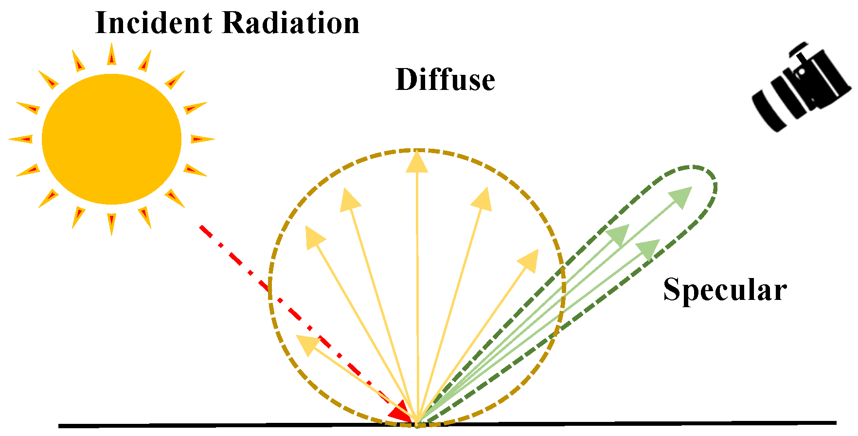
Figure 1 provides an example image representing the diffuse and specular components occurring on the surface of an object. In Equation (
1), the diffuse component is denoted as
, the specular component as
, and the combined intensity as
I.
Here, the diffuse component refers to the light rays that penetrate the surface of an object, undergo multiple reflections and refractions, and are then re-emitted. On the other hand, specular refers to the portion of incoming light rays that are reflected directly, and its intensity varies depending on the roughness of the surface of an object.
Non-learning methods Removing specular highlights has been a subject of research for a long time. Shafer [
14] proposed a dichromatic reflection model to examine the components present on the surface of an object. This model was formulated assuming the object was opaque and inhomogeneous. The dichromatic reflection model has been widely cited and has significantly influenced the field of computer graphics and subsequent research in specular highlight removal.
Klinker
et al. [
15] extended the concepts of the research [
14] by considering that the distribution of pixels on the plane follows a t-shaped color distribution. They proposed an algorithm based on this concept. Bajcsy
et al. [
16] suggested a technique that performs this task in a color domain consisting of lightness, saturation, and hue. On the other hand, these techniques require color segmentation techniques, which can be a significant drawback in complex textures.
Tan and Ikeuchi [
17] aimed to overcome these issues by proposing an effective method that can remove specular highlights without the need for explicit color segmentation. They introduced the specular-to-diffuse mechanism and the concept of a specular-free image containing only the diffuse reflection component. Based on the observation that the specular-free image has the same geometric distribution as the original intensity image, they devised a method to estimate the diffuse reflection through the logarithmic differentiation of the original and specular-free images. This approach significantly influenced further research [
18,
19,
20,
21].
Subsequent research focused heavily on optimization techniques. Kim
et al. [
22] proposed a maximum a-posteriori (MAP) optimization technique based on the observation that the dark channel provides pseudo-specular reflection results in general natural images. Fu
et al. [
23] used k-means clustering and various priors in an optimization technique, and Akashi and Okatani [
24] proposed an optimization technique based on sparse non-negative Matrix factorization (NMF).
Deep learning methods Traditional non-learning methods removed reflection components using handcrafted priors. Nevertheless, one of the drawbacks of handcrafted priors is their lack of robustness in various environments. Recent research has shifted towards data-driven learning approaches to address this issue.
Funke
et al. [
25] proposed a GAN-based network to remove specular highlights from single endoscopic images. Lin
et al. [
26] introduced a new learning method: a fully convolutional neural network (CNN) for generating the diffuse component. Unlike traditional GAN methods, this approach used a multi-class classifier in the discriminator instead of a binary classifier to find more constrained features. Muhammad
et al. [
27] introduced Spec-Net and Spec-CGAN to remove high-intensity specular highlights in low-saturation images, particularly faces.
The deep learning techniques mentioned above can still result in color distortion in areas without specular components. Therefore, research has focused on detecting specular highlight regions and removing only the specular components in these areas. Fu
et al. [
28] proposed a generalized image formation model with region detection and a multi-task network based on it. Wu
et al. [
29] introduced a GAN network that models the mapping relationship between the two component image areas using an attenuation mechanism. Hu
et al. [
30] considered that specular highlight components have peculiar characteristics in the luminance channel and proposed a Mask-Guided Cycle-GAN. Wu
et al. [
31] presented an end-to-end deep learning framework consisting of a highlight detection network and a Unet-Transformer network for highlight removal. On the other hand, mask-guided techniques have limitations in removing large-area specular components.
1.1.2. Datasets for training Deep learning model
As acquiring ideal specular and diffuse components in real-world settings is virtually impossible, constructing datasets has been carried out by constraining the shooting environment or applying constraints. Two datasets have been proposed for training deep learning models for specular highlight removal.
The first dataset, the specular highlight image quadruples (SHIQ) dataset [
28], utilized the MIW dataset [
32] acquired by capturing flashes from various directions, which was publicly available. They obtained reflection-free images from this dataset using existing multi-image-based reflection removal techniques [
3]. They further selected high-quality images from the results. After unifying the specular regions to white, they constructed the dataset by cropping and producing specular region masks, resulting in intensity, diffuse, specular, and mask pairs. The second dataset, the PSD dataset [
29], was constructed from real images using a physically based polarizing filter. They applied linear polarizing filters to the light source and circular polarizing filters to the camera, capturing images with minimal values in the filter regions. This process allowed them to obtain images with removed specular components on the object surface, forming the dataset.
1.2. Reflection removal
1.2.1. Methods
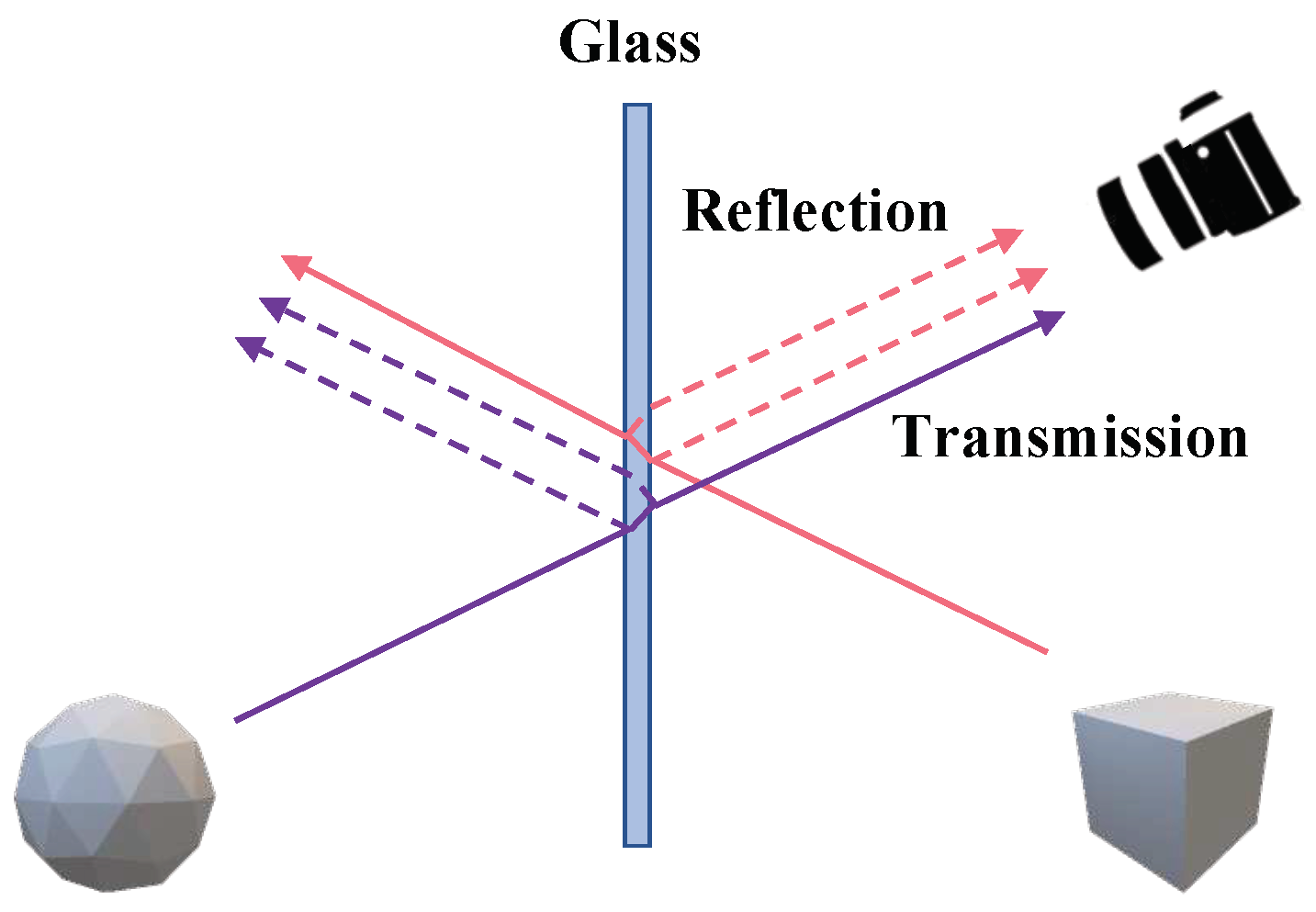
Unlike the problem tackled by specular highlight removal, the primary goal of the reflection removal task is to eliminate reflections occurring in situations with a medium, such as glass, between the object and the viewer and to generate an image of the object that has passed through the glass. In
Figure 2, transmission and reflection represent
and
in Equation (
2).
Each component undergoes transformations depending on the properties of the glass.
is in a state where it has experienced pixel shifts and color alterations due to the refraction and absorption effects of the glass, whereas
is affected by reflection and refraction effects in Equation (
2).
Non-learning method Levin
et al. [
33] is the first proposed method for separating mixed images with reflections using a single image. It introduced an optimization algorithm that minimizes the total amount of edges and corners in the separated images through a prior that they should be minimal. On the other hand, this algorithm was not robust in handling complex pattern images. Removing reflections using a single image is highly ill-posed. Various studies have been conducted based on different priors and assumptions to make it more tractable.
Levin and Weiss [
34] proposed a method that utilizes gradient sparsity priors after users specify a few labels on the image. Li and Brown [
35] used the fact that the camera focus is adjusted for a transmission image, proposing an optimization technique that forces the gradient components of the transmission image to have a long-tailed distribution and those of the reflection image to have a short-tailed distribution. Shih
et al. [
36] modeled the ghost effect using a double-impulse convolution kernel based on the characteristics of ghosting cues. They proposed an algorithm using the Gaussian mixture model (GMM) to separate the layers. Wan
et al. [
37] introduced a multi-scale depth of field (DoF) computation method and separated background and reflection using edge pixel classification based on the computed DoF map. Wan
et al. [
38] used content priors and gradient priors to detect automatically regions with reflections and those without reflections. They proposed an integrated optimization framework for content restoration, background-reflection separation, and missing content restoration.
Deep learning method Owing to the success of deep convolutional neural networks in computer vision tasks compared to non-learning methods, researchers have proposed new data-driven methods for generating robust transmission image predictions for various reflection types. Fan
et al. [
39] introduced the first reflection removal deep learning model that utilizes linear methods to synthesize images with reflections for training and uses edge maps as auxiliary information for guidance. Zhang
et al. [
40] proposed an exclusion loss that minimizes the correlation between the gradient maps of the estimated transmission and reflection layers based on the observation that the edges of transmission and reflection images are unlikely to overlap. Yang
et al. [
41] introduced a deep neural network with a serial structure alternating between estimating reflection and transmission images. Li
et al. [
42] drew inspiration from iterative structure reduction and proposed a continuous network that iteratively refines the estimates of transmission and reflection images using an LSTM module. Zheng
et al. [
43] were inspired by the idea that the absorption effect can be represented numerically by the average of the refraction amplitude coefficient map. They proposed a two-step solution where they estimated the absorption effect from the intensity image and then used the intensity image and the absorption effect as inputs. Dong
et al. [
44] proposed a deep learning model to identify and remove strong reflection locations using multi-scale Laplacian features.
1.2.2. Dataset for training deep learning model
Building a large-scale dataset containing reflection components is a challenging task. Therefore, various strategies have been used to produce training datasets, including generating mixed images by adding reflection and transmission images produced based on mathematical formulae. Alternatively, real-world reflection and transmission images have been acquired separately and combined through linear blending. Some approaches utilize real and synthetic images [
39,
45,
46,
47]. Datasets captured in various environments have been proposed to evaluate the network performance. Among them, the prominent dataset is
[
48].
is categorized into solid objects, postcards, and wild scenes. For solid objects and postcards, the images were captured from seven DoFs and three glass thicknesses in 20 scenes. Wild scenes comprised 100 scenes captured under various settings, including different glass thicknesses, camera settings, and uncontrolled illumination conditions.
2. Proposed Method
This section is structured to explain the methods for constructing the Specular Light (S-Light) dataset, designed to address the removal of specular components occurring in various scenarios, as well as an introduction to the performance metric multi-scale normalized cross-correlation (MS-NCC) to measure the correlation between specular and diffuse components.
2.1. Dataset Construction
The dataset constructed in this study consisted of images containing specular and diffuse components and images containing only the diffuse component.
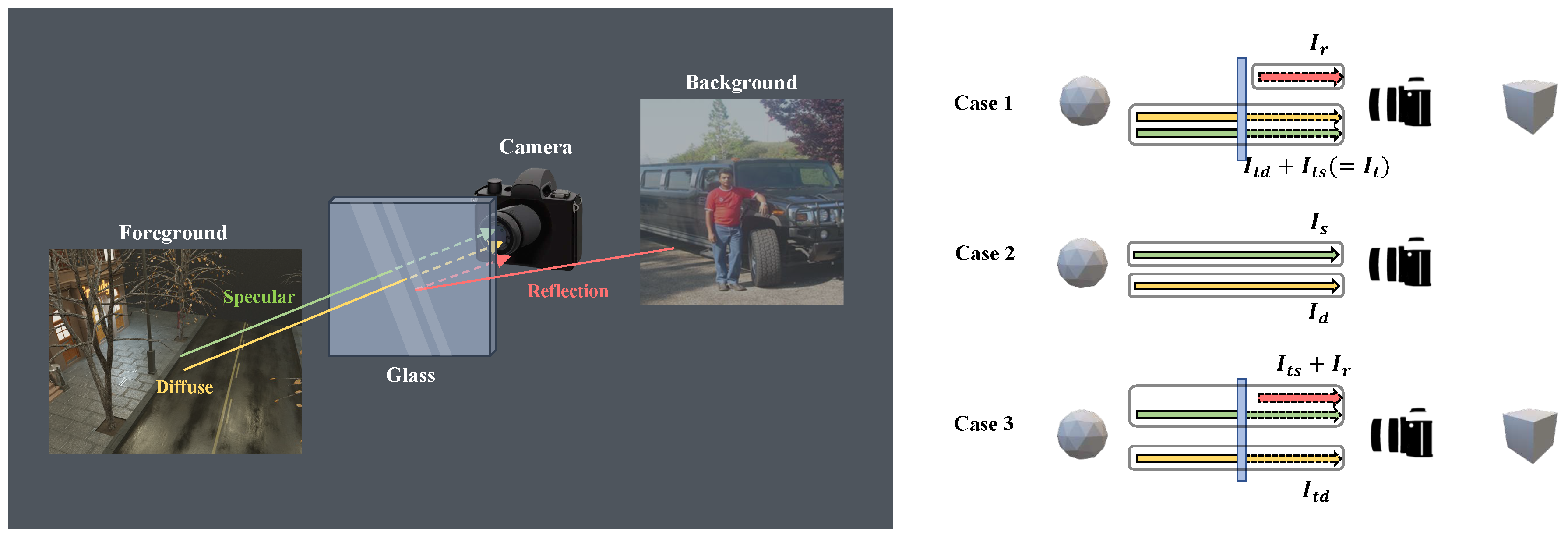
Figure 3 presents Cases 1 and 2, illustrating the problems that reflection removal and specular highlight removal aim to address. In each task, the target consisted of the transmission image
(
) and the diffuse image
. Here,
represents the diffuse component of the transmission image, while
represents the specular component of the transmission image. Case 3 was considered because this paper focused on learning the diffuse component, targeting the transmitted diffuse component in Case 1.
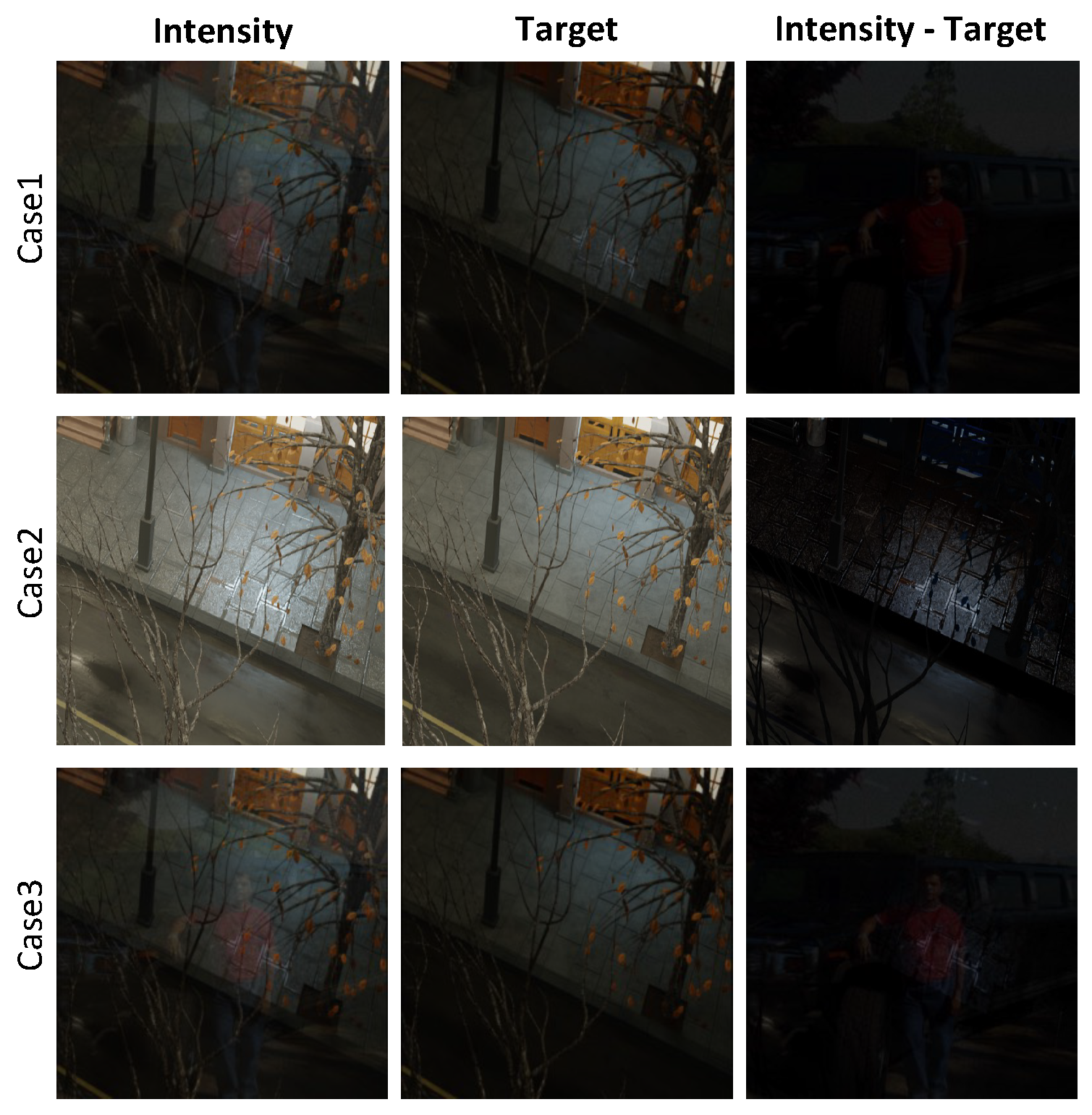
Figure 4 provides example images generated by the research team for each case. A two-step process was used to construct image datasets for Cases 2 and 3. In the first step, the
dataset was constructed. This dataset considers specular reflections originating from object surfaces for Case 2. In the second step, the Case 3 datasets,
and
were constructed using the dataset generated in Step 1. Each subscript in
S-Light represents surface specular, reflection, and combined, respectively.
2.1.1. Step 1 : Construction of Dataset
The SHIQ and PSD datasets consider Case 2 scenarios. On the other hand, existing datasets have the following issues. The SHIQ dataset contains various objects but suffers from specular highlight colors composed only of white, making it less robust to various lighting conditions. PSD, being captured in a controlled laboratory environment, often exhibits mostly black backgrounds or repetitive patterns, and it lacks diversity in the types of objects.
Therefore, 130 multi-object 3D models were collected from the open-source platform Blend Swap [
49] to produce a dataset that includes diverse lighting environments and objects. These models were used in Blend Swap, a free and open-source 3D computer graphics software, using the Path Tracing-based Cycles engine [
49]. Seven hundred and nineteen scenes were generated in rendering scenes where objects and backgrounds do not overlap. Each scene was rendered into intensity and diffuse images at a resolution of
. For data augmentation, the images were cropped randomly to a
resolution or resized, resulting in a dataset of 3,595 pairs.
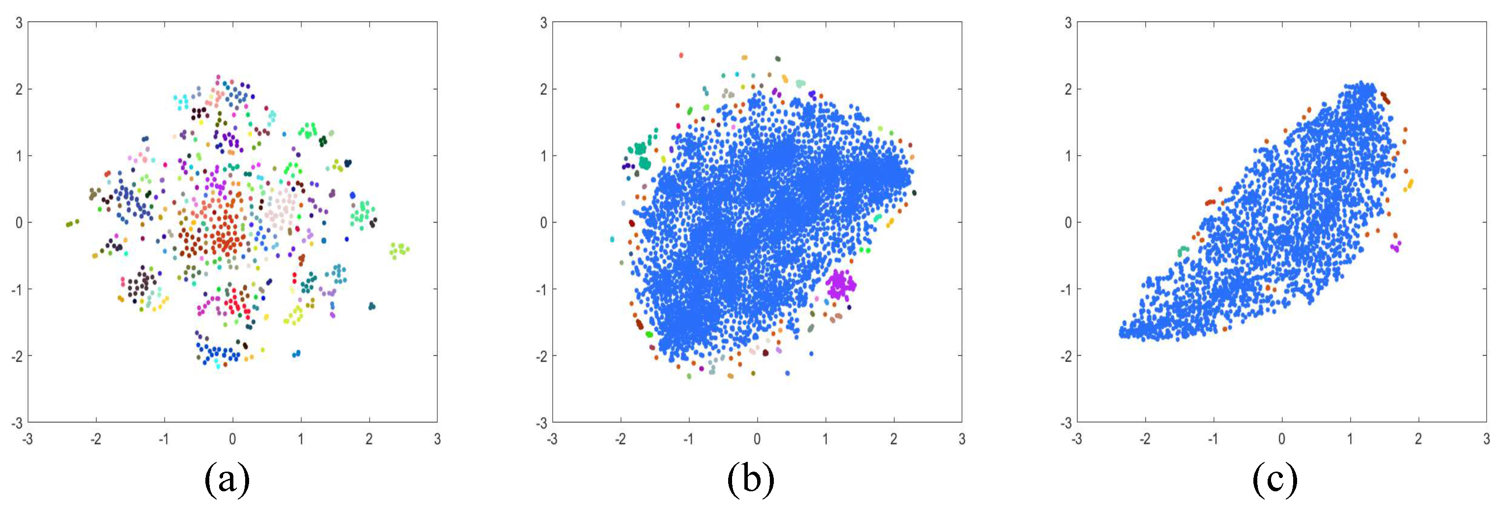
Table 1 presents a quantitative comparison of the existing datasets, SHIQ, PSD, and the dataset developed in this study. I, S, D, and M stand for intensity, specular, diffuse, and mask, respectively. "Clustering portion" indicates the proportion occupied by the largest cluster. Dimensionality reduction into two dimensions using T-SNE [
50] and applying the DBSCAN clustering algorithm [
51] was performed for each dataset to assess the dataset diversity quantitatively.
Figure 5 provides examples of the results of applying the T-SNE and DBSCAN algorithms.
2.1.2. Step 2 : Construction of and Dataset
Previous research has proposed various methods to generate synthetic images and build the reflection-removal dataset. In this study, the techniques reported elsewhere [
45,
46] were applied to generate reflection images. The dataset constructed in Step 1 was used as the transmission image, and the Pascal VOC dataset [
52] was used to render the reflection component.
Kim
et al. [
45] obtained depth images of the image behind the glass and the image reflected on the glass. They proposed a technique that maps the original image onto an object file converted from the depth image to a 3D mesh file for rendering. In this study, the images behind the glass were used for the proposed dataset, and ZoeDepth [
53] was used to render the dataset for obtaining depth maps. Fan
et al. [
39] proposed a technique that applies a Gaussian filter to the reflection data because the reflection images are blurry and have lower intensity than the generated using the same setup. The datasets for Case 1 and Case 3, namely
and
, were also constructed using the dataset from Case 1.
2.2. Multi-Scale NCC
Many researchers have traditionally used performance metrics like the Peak Signal-to-Noise Ratio (PSNR) and the structural similarity index (SSIM) that consider the similarity with reference images to compare the performance of specular highlight and reflection removal deep learning models. On the other hand, there were limitations in expressing the performance of techniques in terms of errors and similarity with reference images because acquiring the diffuse component, excluding the specular highlight from the object surface, is virtually impossible.
The problem addressed in this study was separating or removing integrated specular images from the intensity image. Therefore, performance metrics that consider Cases 2 and 3 are needed. Diffuse and specular components occurring on the object surface are independent, and the independence of diffuse and specular components has been applied widely in non-learning methods [
14,
17]. Transmission and reflection images are also independent scenes from each other. Hence, in general situations, the two components, specular removal and reflection removal, have a low correlation.
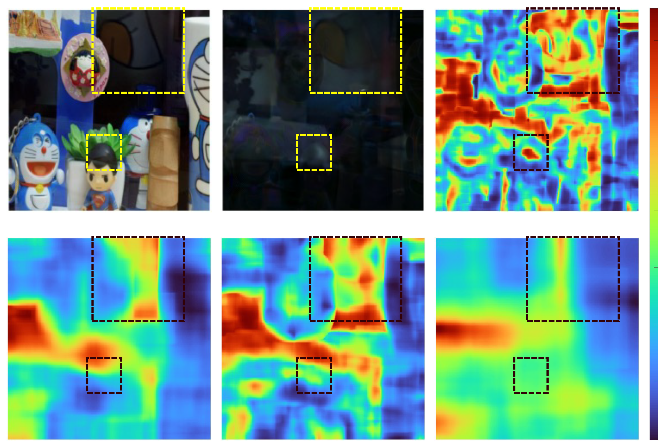
Figure 6 provides example images showing correlation maps based on the window size, depicting the results of applying MS-NCC to the output and residual images of the deep learning model.
The Equation (
6) considers the global independence of the transmission and reflection images and the local independence between the diffuse and specular components within objects. Equation (
3) expresses the average map,
of pixels within a window of odd size (
) in the image
f, where
denotes the pixel coordinates, and the ranges for
u and
v are from
to
.
Equation (
4) presents a formula that indicates the variability in the input image. When the input images are the same, it represents the local variance, whereas it corresponds to the local covariance when the input images are different.
Equation (
5) represents the local normalized cross-correlation (Local-NCC) between the input images,
f and
g, based on their local information.
The window size, denoted as
, is determined based on the smaller dimension of the input image, and this
window size will be the same size as
of the smaller dimension. Multi Scale-NCC was calculated as the weighted sum of Local-NCC, and the weight value
has been uniformly set.
This study evaluated the multi-scale correlations between the output images of the deep learning model and the removed images using MS-NCC.
3. Experiments
There are no reports on a single-image-based deep learning network that simultaneously addresses the removal of specular images on object surfaces and images containing reflections on glass, including transmitted specular components. Therefore, experiments were conducted using models proposed for the existing problems of specular highlight removal and reflection removal. The models used in this experiment are as follows:
- -
Specular Highlight Removal Network: [
29,
30,
31]
- -
Reflection Removal Network: [
42,
43,
54,
55]
3.1. Training and evaluation in specular highlight removal network
This experiment assessed the generalizability of specular highlight removal networks and their suitability for training on the dataset constructed in this study. The common characteristics of the specular highlight removal networks used in the experiment include detecting the removal region and removing the reflection component based on the detected area. Mask images indicating specular locations are required to train detection-based deep learning models. This study did not construct mask images separately for the Case 2 dataset. Therefore, the technique proposed in the SHIQ [
28] paper was applied to produce binary mask images for this dataset. The training and test datasets were split at an 80:20 ratio for the experiment.
Table 2 and
Table 3 present the performance of models trained on each dataset when tested on their respective test datasets. This experiment adopted PSNR, SSIM, NCC, and MS-NCC as the performance metrics. The output image
and the specular image
of the model were used to compute NCC and MS- NCC; both images were converted to grayscale images.
In general, the detection-based specular highlight removal networks used in this experiment showed higher performance on the previously proposed datasets, SHIQ [
28] and PSD [
29], than the dataset constructed in this paper. This trend aligns with expectations. Initially, the SHIQ [
28] and PSD [
29] datasets were constructed assuming that specular images were composed mostly of white highlights or produced in controlled experimental environments using single lighting conditions. As a result, the existing SHIQ [
28] and PSD [
29] datasets share common features that can aid deep learning models in specular region detection training.
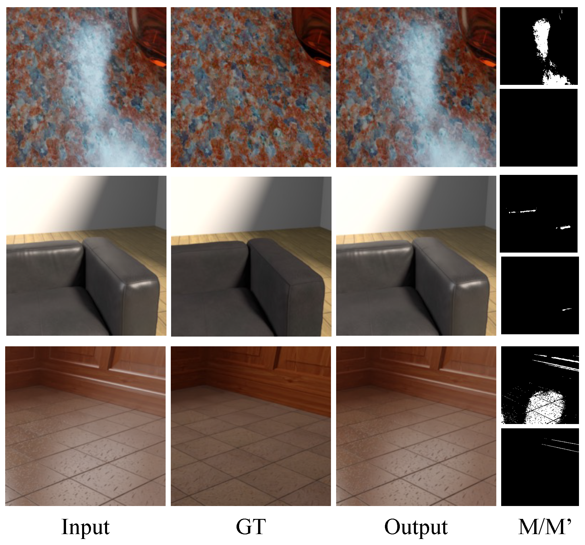
On the other hand, the dataset constructed in this study consisted of various lighting conditions and objects, resulting in a wide range of specular components. Experiments confirmed that specular region detection training was not as effective on the present dataset.
Figure 7 provides examples of models trained with the proposed dataset during testing.
3.2. Training and evaluation in reflection removal network
This experiment assessed the generality of reflection removal networks and their suitability for training with the dataset constructed in this study.
Table 3 summarizes the performance of models trained on each dataset when tested on their respective test datasets, following a similar structure to that in
Table 2. The models trained with the current dataset exhibited better performance across PSNR, SSIM, NCC, and MS-NCC metrics than previously conducted specular removal models.
Furthermore, the NCC and MS-NCC values for the SHIQ [
28] and PSD [
29] test datasets either outperformed or closely matched those trained on the same dataset.
Figure 8 presents example images from the model trained on the present dataset when applied to SHIQ [
28] test images. Several network output images exhibited a more natural appearance and effectively removed specular components occurring on smooth materials, such as glass and metal, compared to the ground truth images.
3.3. Training on the Constructed Dataset and Evaluation on Real Images
This experiment assessed the "trends" in whether the deep learning models trained on the proposed dataset show significant performance in real-world scenarios. An experimental model designed for reflection removal was used to train the dataset proposed in this paper, which considers reflection and surface specular components. Several reasons support this choice. First, experiments A and B showed that a dataset focused solely on surface specular components is suitable for training a reflection removal model.
Second, the models also showed versatility when applied to the [
28] and PSD [
29] test datasets. The reflection components constructed in this paper are present throughout the entire image, making detection-based specular removal networks unsuitable. Two distinct settings were used in the training methodology:
Half Settting : In the first setting, 50% of the data were randomly selected from the and datasets.
Combined Setting : The second setting exclusively involved the use of the dataset.
Table 4 and
Table 5 present the quantitative evaluations of the Wild and Solid Object datasets, respectively. Overall, the correlation between the model output image and the residual image was lower for models trained in the "half" setting compared to the results in the "combined" setting, as indicated by NCC and MS-NCC. Furthermore, there was a significant discrepancy between Zheng [
43] in
Table 4 and Wei [
54] and Zheng [
43] in
Table 5.
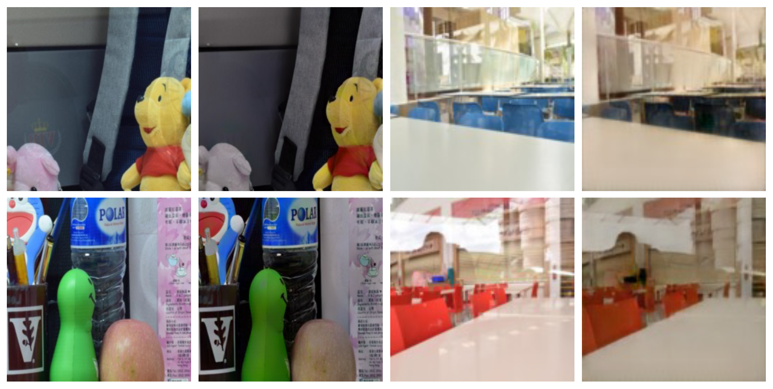
Figure 9 presents the output images of these networks, providing a visual confirmation of specular removal results and color distortion occurrences. In contrast, the half-setting exhibits a robust tendency.
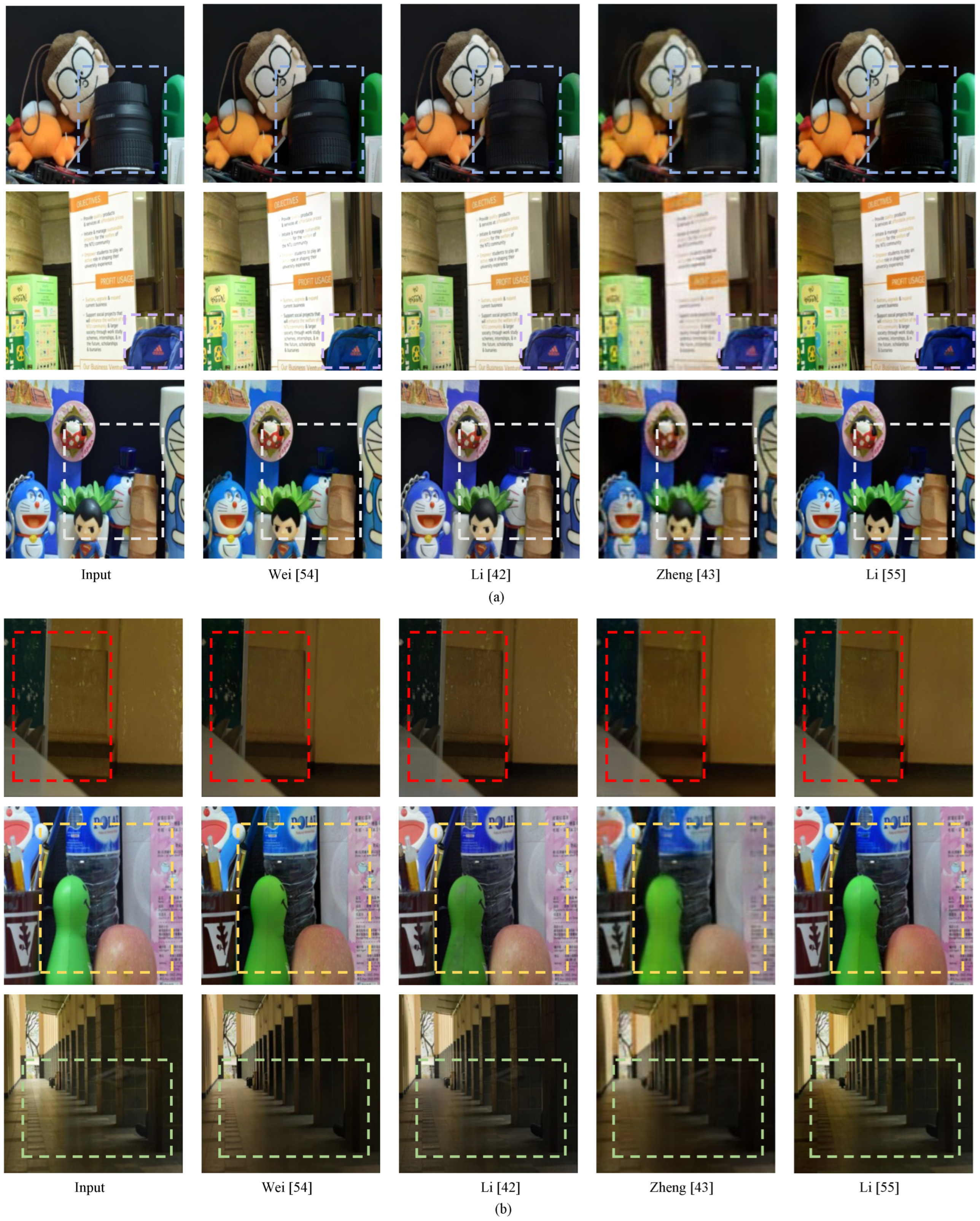
Figure 10 presents the output images from the model trained in the half setting. The images were divided into cases where mix and transmission images from the Wild and Solid Object datasets of
were used as inputs.
In each setting, well-known reflection removal benchmarks were used to evaluate the models on real-world images in Cases 2 and 3: the SIR-Wild and Solid object datasets. The SIR dataset consisted of intensity, transmission, and reflection images. The transmission and intensity images were used for Cases 2 and 3, respectively. NCC and MS-NCC were used as evaluation metrics to compare the correlation between the model output image and the residual image because there are no reference images in the considered scenarios, similar to experiments A and B.
4. Conclusions
Specular reflection removal was categorized into three main scenarios, and a dataset tailored for training single-image-based deep learning models was proposed to address these scenarios. Experiments that were divided into two categories were conducted to investigate suitable networks for the proposed S-Light dataset: one using an area detector-based specular highlight deep learning model and the other using a reflection removal deep learning model. The reflection removal deep learning model trained on the S-Light dataset exhibited generalizability, as confirmed by the previously proposed metrics, such as SHIQ and PSD.
Furthermore, a quantitative measure called MS-NCC, which relies on the correlation between the diffuse and specular components, was used to evaluate the network performance. This measure was effective when applied to real-world images from datasets, such as the Wildscene and Solid object. Therefore, for the effective removal of specular reflections, it is essential to construct an appropriate dataset. Moreover, considering various environmental conditions, a larger dataset will produce more robust results in real-world images.
In conclusion, three major research areas necessary for comprehensive specular removal were addressed. First, the establishment of training datasets was achieved. Second, the research into deep learning models was suitable for integrated specular removal. Finally, benchmark datasets were developed for more detailed quantitative evaluation in real-world scenarios. Future studies will focus on deep learning models that can adapt to and excel in various real-world environments based on the S-Light dataset, unifying the field of specular removal.
References
- Bayoudh, K.; Knani, R.; Hamdaoui, F.; Mtibaa, A. A survey on deep multimodal learning for computer vision: advances, trends, applications, and datasets. The Visual Computer 2021, pp. 1–32.
- Summaira, J.; Li, X.; Shoib, A.M.; Li, S.; Abdul, J. Recent advances and trends in multimodal deep learning: a review. arXiv preprint arXiv:2105.11087 2021.
- Guo, X.; Cao, X.; Ma, Y. Robust separation of reflection from multiple images. Proceedings of the IEEE conference on computer vision and pattern recognition, 2014, pp. 2187–2194.
- Su, T.; Zhou, Y.; Yu, Y.; Du, S. Highlight Removal of Multi-View Facial Images. Sensors 2022, 22, 6656.
- Xue, T.; Rubinstein, M.; Liu, C.; Freeman, W.T. A computational approach for obstruction-free photography. ACM Transactions on Graphics (TOG) 2015, 34, 1–11.
- Li, Y.; Brown, M.S. Exploiting reflection change for automatic reflection removal. Proceedings of the IEEE international conference on computer vision, 2013, pp. 2432–2439.
- Nayar, S.K.; Fang, X.S.; Boult, T. Separation of reflection components using color and polarization. International Journal of Computer Vision 1997, 21, 163–186.
- Umeyama, S.; Godin, G. Separation of diffuse and specular components of surface reflection by use of polarization and statistical analysis of images. IEEE Transactions on Pattern Analysis and Machine Intelligence 2004, 26, 639–647.
- Wen, S.; Zheng, Y.; Lu, F. Polarization guided specular reflection separation. IEEE Transactions on Image Processing 2021, 30, 7280–7291.
- Kong, N.; Tai, Y.W.; Shin, S.Y. High-quality reflection separation using polarized images. IEEE Transactions on Image Processing 2011, 20, 3393–3405.
- Kong, N.; Tai, Y.W.; Shin, J.S. A physically-based approach to reflection separation: from physical modeling to constrained optimization. IEEE transactions on pattern analysis and machine intelligence 2013, 36, 209–221.
- Agrawal, A.; Raskar, R.; Chellappa, R. Edge suppression by gradient field transformation using cross-projection tensors. 2006 IEEE Computer Society Conference on Computer Vision and Pattern Recognition (CVPR’06). IEEE, 2006, Vol. 2, pp. 2301–2308.
- Agrawal, A.; Raskar, R.; Nayar, S.K.; Li, Y. Removing photography artifacts using gradient projection and flash-exposure sampling. In ACM SIGGRAPH 2005 Papers; 2005; pp. 828–835.
- Shafer, S.A. Using color to separate reflection components. Color Research & Application 1985, 10, 210–218.
- Klinker, G.J.; Shafer, S.A.; Kanade, T. The measurement of highlights in color images. International Journal of Computer Vision 1988, 2, 7–32.
- Bajcsy, R.; Lee, S.W.; Leonardis, A. Detection of diffuse and specular interface reflections and inter-reflections by color image segmentation. International Journal of Computer Vision 1996, 17, 241–272.
- Tan, R.T.; Ikeuchi, K. Separating Reflection Components of Textured Surfaces Using a Single Image. IEEE Transactions on pattern analysis and machine intelligence 2005, 27.
- Shen, L.; Machida, T.; Takemura, H. Efficient photometric stereo technique for three-dimensional surfaces with unknown BRDF. Fifth International Conference on 3-D Digital Imaging and Modeling (3DIM’05). IEEE, 2005, pp. 326–333.
- Yoon, K.J.; Choi, Y.; Kweon, I.S. Fast separation of reflection components using a specularity-invariant image representation. 2006 international conference on image processing. IEEE, 2006, pp. 973–976.
- Shen, H.L.; Cai, Q.Y. Simple and efficient method for specularity removal in an image. Applied optics 2009, 48, 2711–2719.
- Yang, Q.; Wang, S.; Ahuja, N. Real-time specular highlight removal using bilateral filtering. Computer Vision–ECCV 2010: 11th European Conference on Computer Vision, Heraklion, Crete, Greece, September 5-11, 2010, Proceedings, Part IV 11. Springer, 2010, pp. 87–100.
- Kim, H.; Jin, H.; Hadap, S.; Kweon, I. Specular reflection separation using dark channel prior. Proceedings of the IEEE conference on computer vision and pattern recognition, 2013, pp. 1460–1467.
- Fu, G.; Zhang, Q.; Song, C.; Lin, Q.; Xiao, C. Specular Highlight Removal for Real-world Images. Computer graphics forum. Wiley Online Library, 2019, Vol. 38, pp. 253–263.
- Akashi, Y.; Okatani, T. Separation of reflection components by sparse non-negative matrix factorization. Computer Vision–ACCV 2014: 12th Asian Conference on Computer Vision, Singapore, Singapore, November 1-5, 2014, Revised Selected Papers, Part V 12. Springer, 2015, pp. 611–625.
- Funke, I.; Bodenstedt, S.; Riediger, C.; Weitz, J.; Speidel, S. Generative adversarial networks for specular highlight removal in endoscopic images. Medical Imaging 2018: Image-Guided Procedures, Robotic Interventions, and Modeling. SPIE, 2018, Vol. 10576, pp. 8–16.
- Lin, J.; El Amine Seddik, M.; Tamaazousti, M.; Tamaazousti, Y.; Bartoli, A. Deep multi-class adversarial specularity removal. Image Analysis: 21st Scandinavian Conference, SCIA 2019, Norrköping, Sweden, June 11–13, 2019, Proceedings 21. Springer, 2019, pp. 3–15.
- Muhammad, S.; Dailey, M.N.; Farooq, M.; Majeed, M.F.; Ekpanyapong, M. Spec-Net and Spec-CGAN: Deep learning models for specularity removal from faces. Image and Vision Computing 2020, 93, 103823.
- Fu, G.; Zhang, Q.; Zhu, L.; Li, P.; Xiao, C. A multi-task network for joint specular highlight detection and removal. Proceedings of the IEEE/CVF Conference on Computer Vision and Pattern Recognition, 2021, pp. 7752–7761.
- Wu, Z.; Zhuang, C.; Shi, J.; Guo, J.; Xiao, J.; Zhang, X.; Yan, D.M. Single-image specular highlight removal via real-world dataset construction. IEEE Transactions on Multimedia 2021, 24, 3782–3793.
- Hu, G.; Zheng, Y.; Yan, H.; Hua, G.; Yan, Y. Mask-guided cycle-GAN for specular highlight removal. Pattern Recognition Letters 2022, 161, 108–114.
- Wu, Z.; Guo, J.; Zhuang, C.; Xiao, J.; Yan, D.M.; Zhang, X. Joint specular highlight detection and removal in single images via Unet-Transformer. Computational Visual Media 2023, 9, 141–154.
- Murmann, L.; Gharbi, M.; Aittala, M.; Durand, F. A dataset of multi-illumination images in the wild. Proceedings of the IEEE/CVF International Conference on Computer Vision, 2019, pp. 4080–4089.
- Levin, A.; Zomet, A.; Weiss, Y. Separating reflections from a single image using local features. Proceedings of the 2004 IEEE Computer Society Conference on Computer Vision and Pattern Recognition, 2004. CVPR 2004. IEEE, 2004, Vol. 1, pp. I–I.
- Levin, A.; Weiss, Y. User assisted separation of reflections from a single image using a sparsity prior. IEEE Transactions on Pattern Analysis and Machine Intelligence 2007, 29, 1647–1654.
- Li, Y.; Brown, M.S. Single image layer separation using relative smoothness. Proceedings of the IEEE Conference on Computer Vision and Pattern Recognition, 2014, pp. 2752–2759.
- Shih, Y.; Krishnan, D.; Durand, F.; Freeman, W.T. Reflection removal using ghosting cues. Proceedings of the IEEE conference on computer vision and pattern recognition, 2015, pp. 3193–3201.
- Wan, R.; Shi, B.; Hwee, T.A.; Kot, A.C. Depth of field guided reflection removal. 2016 IEEE International Conference on Image Processing (ICIP). IEEE, 2016, pp. 21–25.
- Wan, R.; Shi, B.; Duan, L.Y.; Tan, A.H.; Gao, W.; Kot, A.C. Region-aware reflection removal with unified content and gradient priors. IEEE Transactions on Image Processing 2018, 27, 2927–2941.
- Fan, Q.; Yang, J.; Hua, G.; Chen, B.; Wipf, D. A generic deep architecture for single image reflection removal and image smoothing. Proceedings of the IEEE International Conference on Computer Vision, 2017, pp. 3238–3247.
- Zhang, X.; Ng, R.; Chen, Q. Single image reflection separation with perceptual losses. Proceedings of the IEEE conference on computer vision and pattern recognition, 2018, pp. 4786–4794.
- Yang, J.; Gong, D.; Liu, L.; Shi, Q. Seeing deeply and bidirectionally: A deep learning approach for single image reflection removal. Proceedings of the european conference on computer vision (ECCV), 2018, pp. 654–669.
- Li, C.; Yang, Y.; He, K.; Lin, S.; Hopcroft, J.E. Single image reflection removal through cascaded refinement. Proceedings of the IEEE/CVF Conference on Computer Vision and Pattern Recognition, 2020, pp. 3565–3574.
- Zheng, Q.; Shi, B.; Chen, J.; Jiang, X.; Duan, L.Y.; Kot, A.C. Single image reflection removal with absorption effect. Proceedings of the IEEE/CVF Conference on Computer Vision and Pattern Recognition, 2021, pp. 13395–13404.
- Dong, Z.; Xu, K.; Yang, Y.; Bao, H.; Xu, W.; Lau, R.W. Location-aware single image reflection removal. Proceedings of the IEEE/CVF international conference on computer vision, 2021, pp. 5017–5026.
- Kim, S.; Huo, Y.; Yoon, S.E. Single image reflection removal with physically-based training images. Proceedings of the IEEE/CVF conference on computer vision and pattern recognition, 2020, pp. 5164–5173.
- Ma, D.; Wan, R.; Shi, B.; Kot, A.C.; Duan, L.Y. Learning to jointly generate and separate reflections. Proceedings of the IEEE/CVF International Conference on Computer Vision, 2019, pp. 2444–2452.
- Wan, R.; Shi, B.; Li, H.; Duan, L.Y.; Tan, A.H.; Kot, A.C. CoRRN: Cooperative reflection removal network. IEEE transactions on pattern analysis and machine intelligence 2019, 42, 2969–2982.
- Wan, R.; Shi, B.; Duan, L.Y.; Tan, A.H.; Kot, A.C. Benchmarking single-image reflection removal algorithms. Proceedings of the IEEE International Conference on Computer Vision, 2017, pp. 3922–3930.
- Blend Swap. https://www.blendswap.com/.
- Van der Maaten, L.; Hinton, G. Visualizing data using t-SNE. Journal of machine learning research 2008, 9.
- Ester, M.; Kriegel, H.P.; Sander, J.; Xu, X.; others. A density-based algorithm for discovering clusters in large spatial databases with noise. kdd, 1996, Vol. 96, pp. 226–231.
- Everingham, M.; Van Gool, L.; Williams, C.K.; Winn, J.; Zisserman, A. The pascal visual object classes (voc) challenge. International journal of computer vision 2010, 88, 303–338.
- Bhat, S.F.; Birkl, R.; Wofk, D.; Wonka, P.; Müller, M. ZoeDepth: Zero-shot Transfer by Combining Relative and Metric Depth, 2023. [CrossRef]
- Wei, K.; Yang, J.; Fu, Y.; David, W.; Huang, H. Single Image Reflection Removal Exploiting Misaligned Training Data and Network Enhancements. IEEE Conference on Computer Vision and Pattern Recognition, 2019.
- Li, Y.; Liu, M.; Yi, Y.; Li, Q.; Ren, D.; Zuo, W. Two-stage single image reflection removal with reflection-aware guidance. Applied Intelligence 2023, 53, 1–16. [CrossRef]
Figure 1.
Diffuse and specular reflection occurring on the surface of an object.
Figure 1.
Diffuse and specular reflection occurring on the surface of an object.
Figure 2.
Diffuse and glass reflection.
Figure 2.
Diffuse and glass reflection.
Figure 3.
(Left) Example image illustrating the captured reflection component from the camera. (Right) Cases 1 and 2 briefly represent the problems that reflection removal and specular highlight removal aim to address. Case 3 is an extension of Case 1, where the target is the diffuse component.
Figure 3.
(Left) Example image illustrating the captured reflection component from the camera. (Right) Cases 1 and 2 briefly represent the problems that reflection removal and specular highlight removal aim to address. Case 3 is an extension of Case 1, where the target is the diffuse component.
Figure 4.
Example images from the proposed dataset.
Figure 4.
Example images from the proposed dataset.
Figure 5.
Results of applying T-SNE and DBSCAN clustering: (a) PSD dataset, (b) SHIQ dataset, and (c) dataset.
Figure 5.
Results of applying T-SNE and DBSCAN clustering: (a) PSD dataset, (b) SHIQ dataset, and (c) dataset.
Figure 6.
In the z-direction, model output image, residual image, and correlation map from the small to large window application.
Figure 6.
In the z-direction, model output image, residual image, and correlation map from the small to large window application.
Figure 7.
Example images from the region detection-based model [
29] M/M’ represents Mask GT (Ground Truth) and Mask Output in each row.
Figure 7.
Example images from the region detection-based model [
29] M/M’ represents Mask GT (Ground Truth) and Mask Output in each row.
Figure 8.
Examples of specular removal results on the SHIQ test set after training the dataset. (GT: Ground Truth).
Figure 8.
Examples of specular removal results on the SHIQ test set after training the dataset. (GT: Ground Truth).
Figure 9.
Color distortion example. Odd columns : input images, Even columns : output images.
Figure 9.
Color distortion example. Odd columns : input images, Even columns : output images.
Figure 10.
Half setting model results: (a) Input and output images of Case 3, (b) Input and output images of Case 2.
Figure 10.
Half setting model results: (a) Input and output images of Case 3, (b) Input and output images of Case 2.
Table 1.
Seven hundred and nineteen scenes were generated in rendering scenes where the objects and backgrounds do not overlap. (I, S, D, and M stand for Intensity, Specular, Diffuse, and Mask).
Table 1.
Seven hundred and nineteen scenes were generated in rendering scenes where the objects and backgrounds do not overlap. (I, S, D, and M stand for Intensity, Specular, Diffuse, and Mask).
| |
Number of
Images |
Image
Set |
Specular
Color |
Clustering
Portion |
Scene |
Acquisition |
| PSD [29] |
13,380 |
I,D |
Multiple |
0.007 |
2,210 |
Captured |
| SHIQ [28] |
10,825 |
I,D,S,M |
Single |
0.9 |
1,016 |
Captured
+RPCA[3] |
|
S-Light
|
3,595 |
I,D |
Multiple |
0.96 |
719 |
Rendering |
Table 2.
Evaluation of specular highlight removal models trained on each dataset when assessed on the corresponding test datasets. The training dataset is indicated next to the model names on the right. The test dataset is listed at the top. When the training and test datasets differ, they are highlighted in green. "Mean" represents the average value within the highlighted green area. The best-performing values for each model/test dataset combination are shown in bold.
| |
|
S-Light (Proposed DB) |
SHIQ [28] |
PSD [29] |
Mean |
| |
|
PSNR ↑ |
SSIM ↑ |
NCC ↓ |
MS-NCC ↓ |
PSNR ↑ |
SSIM ↑ |
NCC ↓ |
MS-NCC ↓ |
PSNR ↑ |
SSIM ↑ |
NCC ↓ |
MS-NCC ↓ |
PSNR ↑ |
SSIM ↑ |
NCC ↓ |
MS-NCC ↓ |
| |
S-Light
|
15.895 |
0.666 |
0.614 |
0.468 |
19.954 |
0.861 |
0.643 |
0.728 |
17.417 |
0.754 |
0.731 |
0.872 |
18.685 |
0.807 |
0.687 |
0.800 |
| |
SHIQ [28] |
22.657 |
0.785 |
0.512 |
0.498 |
30.754 |
0.950 |
0.285 |
0.581 |
23.931 |
0.888 |
0.446 |
0.516 |
23.294 |
0.837 |
0.479 |
0.507 |
| Wu [31] |
PSD [29] |
24.143 |
0.844 |
0.235 |
0.324 |
24.374 |
0.908 |
0.249 |
0.231 |
29.049 |
0.951 |
0.201 |
0.215 |
24.258 |
0.876 |
0.242 |
0.277 |
| |
S-Light
|
25.372 |
0.868 |
0.309 |
0.419 |
25.817 |
0.927 |
0.321 |
0.459 |
28.113 |
0.946 |
0.111 |
0.110 |
26.965 |
0.936 |
0.216 |
0.284 |
| |
SHIQ [28] |
24.590 |
0.844 |
0.310 |
0.271 |
32.551 |
0.961 |
0.180 |
0.292 |
25.919 |
0.930 |
0.256 |
0.262 |
25.254 |
0.887 |
0.283 |
0.266 |
| Wu [29] |
PSD [29] |
25.870 |
0.862 |
0.150 |
0.166 |
26.971 |
0.929 |
0.175 |
0.163 |
30.155 |
0.958 |
0.137 |
0.130 |
26.420 |
0.895 |
0.162 |
0.165 |
| |
S-Light
|
24.575 |
0.825 |
0.196 |
0.285 |
22.732 |
0.863 |
0.407 |
0.454 |
25.398 |
0.892 |
0.189 |
0.229 |
24.065 |
0.877 |
0.298 |
0.342 |
| |
SHIQ [28] |
21.475 |
0.776 |
0.398 |
0.517 |
27.286 |
0.944 |
0.192 |
0.345 |
24.360 |
0.901 |
0.176 |
0.208 |
22.917 |
0.839 |
0.287 |
0.362 |
| Hu [30] |
PSD [29] |
21.102 |
0.794 |
0.351 |
0.499 |
21.09 |
0.862 |
0.435 |
0.719 |
24.631 |
0.890 |
0.187 |
0.267 |
21.09 |
0.828 |
0.393 |
0.609 |
Table 3.
Evaluation of reflection removal models trained on each dataset when assessed on the corresponding test datasets. The training dataset is indicated next to the model names on the right. This table is identical in structure to
Table 2.
Table 3.
Evaluation of reflection removal models trained on each dataset when assessed on the corresponding test datasets. The training dataset is indicated next to the model names on the right. This table is identical in structure to
Table 2.
| |
|
S-Light (Proposed DB) |
SHIQ [28] |
PSD [29] |
Mean |
| |
|
PSNR ↑ |
SSIM ↑ |
NCC ↓ |
MS-NCC ↓ |
PSNR ↑ |
SSIM ↑ |
NCC ↓ |
MS-NCC ↓ |
PSNR ↑ |
SSIM ↑ |
NCC ↓ |
MS-NCC ↓ |
PSNR ↑ |
SSIM ↑ |
NCC ↓ |
MS-NCC ↓ |
| |
S-Light
|
27.869 |
0.898 |
0.184 |
0.225 |
23.621 |
0.890 |
0.224 |
0.248 |
26.030 |
0.921 |
0.100 |
0.203 |
24.826 |
0.906 |
0.162 |
0.225 |
| |
SHIQ [28] |
23.518 |
0.810 |
0.569 |
0.372 |
32.217 |
0.960 |
0.478 |
0.452 |
22.809 |
0.886 |
0.497 |
0.324 |
23.164 |
0.848 |
0.533 |
0.348 |
| Wei [54] |
PSD [29] |
24.824 |
0.850 |
0.211 |
0.283 |
26.011 |
0.918 |
0.241 |
0.284 |
29.815 |
0.957 |
0.178 |
0.147 |
25.418 |
0.884 |
0.226 |
0.284 |
| |
S-Light
|
16.602 |
0.528 |
0.388 |
0.464 |
12.685 |
0.490 |
0.535 |
0.350 |
13.844 |
0.560 |
0.504 |
0.520 |
13.265 |
0.525 |
0.520 |
0.435 |
| |
SHIQ [28] |
24.761 |
0.844 |
0.209 |
0.452 |
32.634 |
0.964 |
0.200 |
0.418 |
26.500 |
0.928 |
0.248 |
0.533 |
25.630 |
0.886 |
0.229 |
0.492 |
| Li [42] |
PSD [29] |
24.351 |
0.853 |
0.170 |
0.405 |
24.297 |
0.919 |
0.283 |
0.382 |
27.593 |
0.949 |
0.083 |
0.322 |
24.324 |
0.885 |
0.226 |
0.394 |
| |
S-Light
|
27.162 |
0.867 |
0.266 |
0.247 |
25.054 |
0.890 |
0.175 |
0.249 |
24.619 |
0.886 |
0.118 |
0.213 |
24.837 |
0.888 |
0.147 |
0.231 |
| |
SHIQ [28] |
24.192 |
0.805 |
0.368 |
0.372 |
35.309 |
0.965 |
0.141 |
0.342 |
24.729 |
0.897 |
0.334 |
0.386 |
24.460 |
0.851 |
0.351 |
0.379 |
| Zheng [43] |
PSD [29] |
18.177 |
0.719 |
0.355 |
0.344 |
18.586 |
0.764 |
0.326 |
0.511 |
21.762 |
0.918 |
0.197 |
0.172 |
18.382 |
0.742 |
0.340 |
0.427 |
| |
S-Light
|
25.767 |
0.850 |
0.241 |
0.229 |
25.354 |
0.926 |
0.170 |
0.213 |
24.907 |
0.926 |
0.133 |
0.178 |
25.130 |
0.926 |
0.151 |
0.195 |
| |
SHIQ [28] |
22.491 |
0.797 |
0.231 |
0.173 |
30.491 |
0.958 |
0.210 |
0.234 |
22.440 |
0.900 |
0.175 |
0.294 |
22.465 |
0.848 |
0.203 |
0.234 |
| Li [55] |
PSD [29] |
23.787 |
0.833 |
0.222 |
0.227 |
23.386 |
0.910 |
0.222 |
0.309 |
28.872 |
0.957 |
0.131 |
0.188 |
23.586 |
0.872 |
0.222 |
0.268 |
Table 4.
Validation results in Wildscene. M and T represent the Mix and Transmission image sets. Results with better performance in the Half and Combined settings are indicated in bold.
Table 4.
Validation results in Wildscene. M and T represent the Mix and Transmission image sets. Results with better performance in the Half and Combined settings are indicated in bold.
| Model |
|
Wildscene M [48] |
Wildscene T [48] |
| |
NCC |
MS-NCC |
NCC |
MS-NCC |
| Wei [54] |
Half |
0.1437 |
0.2496 |
0.1547 |
0.2129 |
| Combined |
0.1618 |
0.2153 |
0.1474 |
0.2029 |
| Li [42] |
Half |
0.1301 |
0.2376 |
0.1469 |
0.2451 |
| Combined |
0.1277 |
0.1738 |
0.1225 |
0.1659 |
| Zheng [43] |
Half |
0.1284 |
0.2019 |
0.1382 |
0.2023 |
| Combined |
0.1441 |
0.2589 |
0.1433 |
0.2588 |
| Li [55] |
Half |
0.1667 |
0.1549 |
0.1689 |
0.1786 |
| Combined |
0.1484 |
0.2059 |
0.1438 |
0.2578 |
Table 5.
Validation results in Solid object. M and T represent the Mix and Transmission image sets. Results with better performance in the Half and Combined settings are indicated in bold.
Table 5.
Validation results in Solid object. M and T represent the Mix and Transmission image sets. Results with better performance in the Half and Combined settings are indicated in bold.
| Model |
|
Solid Object M [48] |
Solid Object T [48] |
| |
NCC |
MS-NCC |
NCC |
MS-NCC |
| Wei [54] |
Half |
0.1181 |
0.1712 |
0.1588 |
0.1375 |
| Combined |
0.2638 |
0.2744 |
0.2472 |
0.3444 |
| Li [42] |
Half |
0.1271 |
0.1610 |
0.1555 |
0.1254 |
| Combined |
0.1448 |
0.1668 |
0.1991 |
0.2100 |
| Zheng [43] |
Half |
0.1161 |
0.1267 |
0.1229 |
0.1395 |
| Combined |
0.1497 |
0.2650 |
0.1649 |
0.3547 |
| Li [55] |
Half |
0.1376 |
0.1448 |
0.0842 |
0.1354 |
| Combined |
0.1071 |
0.2082 |
0.1229 |
0.1467 |
|
Disclaimer/Publisher’s Note: The statements, opinions and data contained in all publications are solely those of the individual author(s) and contributor(s) and not of MDPI and/or the editor(s). MDPI and/or the editor(s) disclaim responsibility for any injury to people or property resulting from any ideas, methods, instructions or products referred to in the content. |
© 2023 by the authors. Licensee MDPI, Basel, Switzerland. This article is an open access article distributed under the terms and conditions of the Creative Commons Attribution (CC BY) license (http://creativecommons.org/licenses/by/4.0/).
