1. Introduction
Seismic waveform inversion is an essential geophysical method that enables the inversion of physical parameters of the subsurface medium, such as velocity, density, and elastic moduli, from seismic data[
1]. These parameters are of great significance in fields such as oil and gas exploration, earthquake hazard assessment, and geological structure analysis[
2]. However, seismic waveform inversion is also a non-linear, multi-modal, non-convex optimization problem and faces various challenges, such as dependency on initial models, susceptibility to local minima traps, and high computational complexity[
3].
To overcome these challenges, deep learning techniques have been introduced to seismic inversion. Röth and Tarantola were the first to propose the use of neural networks to transform time-domain seismic data into acoustic velocity models in 1994[
4]. Nath et al., in 1999, trained neural networks with synthetic data, resulting in networks capable of estimating formation velocities using inter-well data[
5,
6]. In 2019, Yang and Ma developed a fully convolutional neural network for inverting P-wave velocity models from raw seismic data[
7]. A commonality among these networks is the need for extensive labeled data for training, and once trained, the neural networks can be used as inversion solvers. However, in the field of seismic exploration, acquiring a large labeled dataset is challenging.
Physics-Embedded Neural Networks (PINNs) offer a novel approach to seismic velocity modeling[
8]. The fundamental idea behind PINNs is to use neural networks to approximate unknown functions or parameters and incorporate the residuals of physical equations as part of the loss function. The neural networks are trained by minimizing this loss function, resulting in solutions that satisfy physical constraints[
9]. Moseley et al. (2020) utilized PINNs as solvers for acoustic wave forward propagation[
10,
11], while Smith et al.[
12] and Waheed et al.[
13] applied PINNs to the Eikonal equation for first-arrival prediction and travel-time tomography, respectively. Song et al. employed PINNs to solve the frequency-domain anisotropic acoustic wave equation[
14]. Additionally, PINNs have been successfully used for forward and inverse analyses of various complex systems in cases with limited sensor measurements[
15,
16,
17,
18,
19,
20] or without labeled data[
21,
22,
23,
24,
25].
This paper utilizes Recurrent Neural Networks (RNNs) to simulate the 2D time-domain finite difference acoustic wave equation as the forward process and treats velocity as a network parameter. The velocity model is updated during the backward propagation of the network. This approach enables the integration of information from the acoustic wave equation into the network, guiding the optimization direction of the network, and avoiding explicit solutions for wavefields and gradients, thereby reducing computational costs. Furthermore, it leverages the non-linear fitting capabilities of neural networks to enhance inversion accuracy and robustness. Additionally, given the temporal causality in wavefields, where the current computed wavefield is related to previous wavefields, this paper adopts a time-lapse inversion approach. This ensures that the residuals of the wavefields are minimized at each timestep, guaranteeing the accuracy of subsequent wavefield computations and alleviating the non-uniqueness issue in velocity inversion. The effectiveness and superiority of the method proposed in this paper are verified through numerical experiments.
2. Materials and Methods
2.1. Finite-difference Acoustic Wave Equation
The numerical simulation of wave equation forward modeling is fundamental to inversion. The time-space domain finite difference algorithm is widely used in geophysical forward modeling due to its simplicity and high computational efficiency, and it is employed to simulate the propagation of seismic waves. In the process of solving partial differential wave equations using the finite difference method, the computation area is first discretized into a grid, then grid differences are utilized to approximate the derivative operators, and the wave equation is converted into a difference equation.
In a 2D isotropic acoustic medium, the time-domain wave equation is:
where,
represents the pressure or displacement at coordinate
r at time
t,
represents the speed of sound at coordinate
r,
represents the source function at coordinate
r at time
t, and
is a Dirac (Delta) function, indicating that energy is released only at the source position.
For the 2D medium, spatial discretization is done by converting coordinates (x, y) into grid points (i, j), where i represents the index in the x direction, and j represents the index in the y direction. Uniform grid division is usually adopted, dividing the space into a series of equal-sized cells. Time t is discretized into time steps Δt, allowing time to progress in fixed intervals. Based on discrete spatial grids and time steps, difference approximations are used to replace derivative terms. A centered difference approximation is used to approximate the second-order spatial derivative
:
where Δx and Δy represent the grid spacing in the x and y directions, respectively.
A second-order centered difference approximation is used to approximate the second-order time derivative
:
Substituting the difference approximations into the original wave equation yields the 2D time-domain finite difference acoustic wave equation:
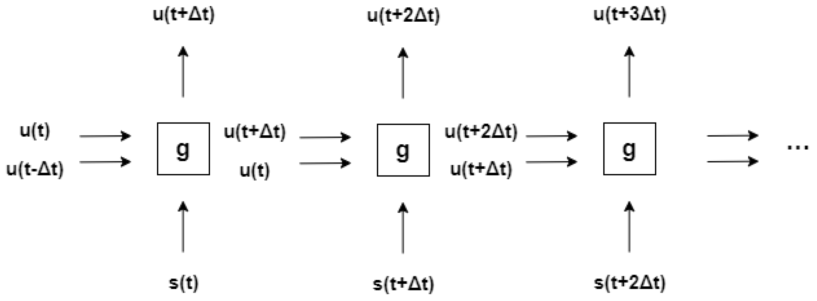
Through the difference acoustic wave equation, the wavefield at the current time can be calculated using the wavefields of the past two time steps, the source, and the velocity model. This relationship can be seen as a function g:
The wavefield at each moment can be considered as part of the time series data. The calculation process of the difference acoustic wave equation is shown in
Figure 1 and
Figure 2.
2.2. Recurrent Neural Network with Acoustic Wave Equation Embedding
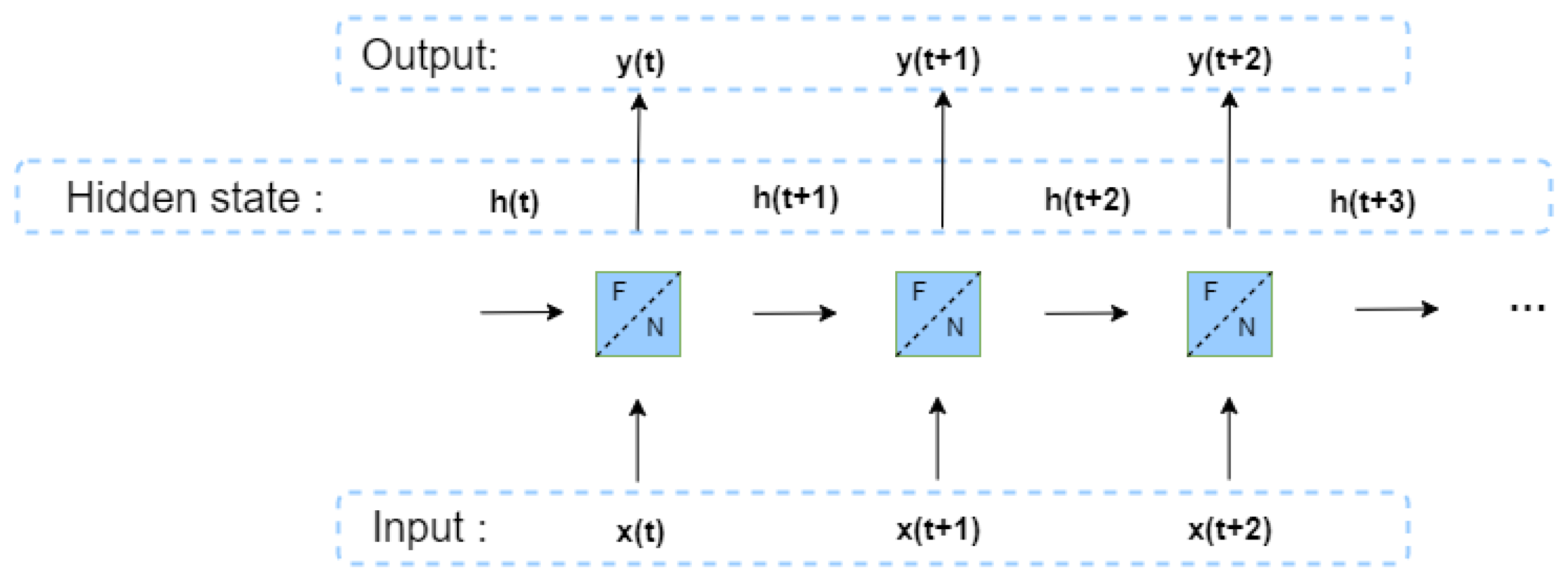
The structure of the RNN (Recurrent Neural Network) is shown in
Figure 3. By comparison, it can be observed that the propagation structure of the difference wave equation has high similarity with the network structure of the RNN, and existing experiments indicate that the dynamics of the wave equation are conceptually equivalent to the RNN. Therefore, the acoustic difference equation can be embedded into the RNN structure, which enables a better understanding of the propagation characteristics of waves and maps them into the neural network structure [
26].
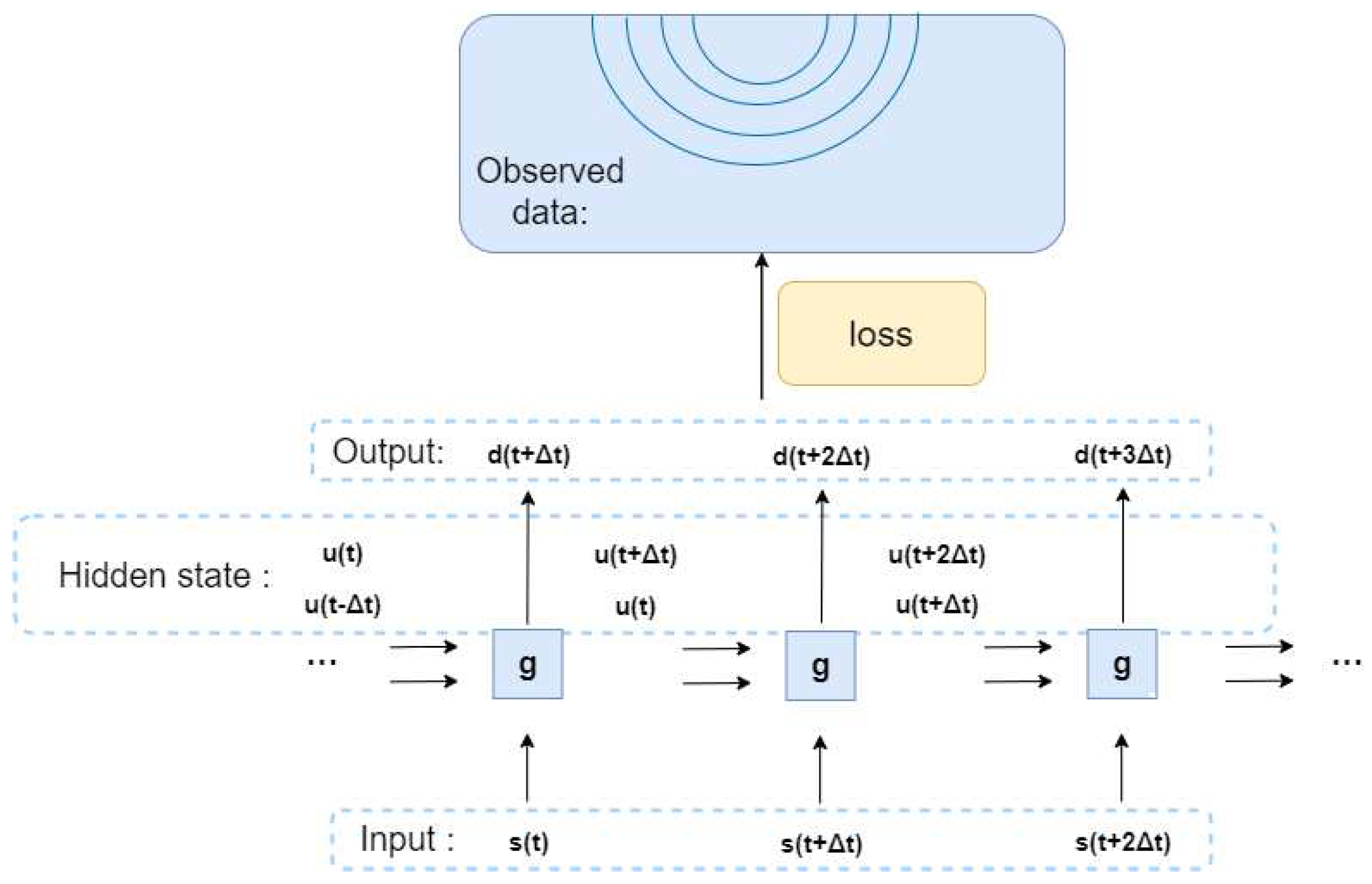
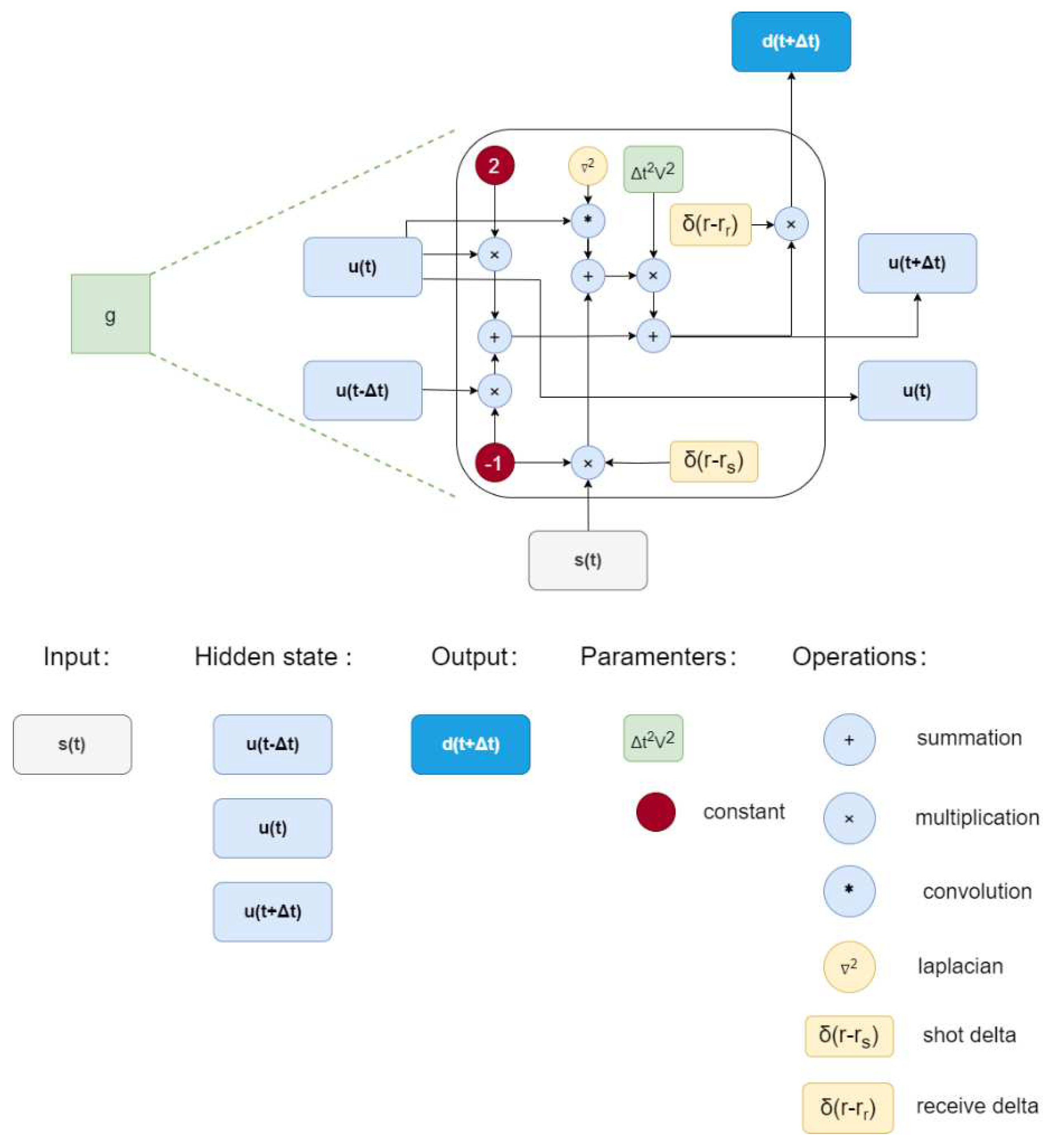
Considering the dependence of the acoustic difference equation on the wavefields of the two previous time steps, these wavefields can be used as hidden states in the RNN. The source function at the current time step can be used as input, and the signal at the detector position for each time step 't' can be used as the shot gather at time 't'. The velocity model in the difference equation can be treated as a trainable parameter within the network. By using the error between the observed and predicted values for backward correction, this process can be viewed as the inversion of the velocity model.
This approach allows the information from the acoustic wave equation to be incorporated into the network, guiding the optimization direction of the network, and avoiding the explicit calculation of gradients, which reduces computational costs. Additionally, the non-linear fitting capabilities of neural networks can be leveraged to improve inversion accuracy and robustness.
The structure of the RNN with embedded difference acoustic wave equation and the structure of operators are shown in
Figure 4 and
Figure 5, respectively.
2.3. Time-by-Time Inversion Algorithm
In RNNs, two common network updating algorithms are generally employed: (1) Compute the loss and update the network at each time step: At each time step, the loss is computed and used to update the network parameters. This is a traditional time-based loss update method. (2) Compute the loss at each time step, sum them, and then update the network: At each time step, the current loss is computed and accumulated with losses from previous time steps. The network parameters are then updated using the accumulated sum of losses. This method integrates information from previous time steps into the current time step loss to provide global information.
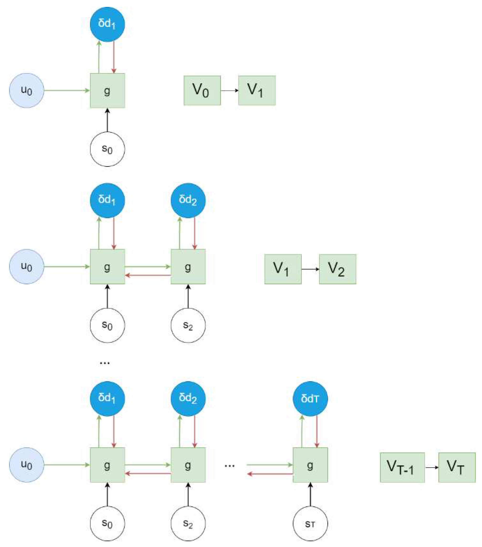
In the RNN embedded with the acoustic wave equation, updating the network by computing the loss at each time step would result in changing the velocity model at different time steps. According to the calculation formula of the difference wave equation (5), the velocity needs to remain consistent throughout the process of solving the acoustic wave equation. Therefore, computing the loss and updating the parameters separately at each time step would violate the constraints of the acoustic wave equation, leading to the inversion not converging. The article introduces a new network loss update method called the step-by-step inversion algorithm. Considering the causality of wavefield propagation, the calculation of the wavefield at the current time step is related to the previous wavefields. If errors are present in the calculation of the preceding wavefields, it will introduce additional errors in the subsequent wavefield calculations. Therefore, it is necessary to ensure the correctness of the preceding wavefield calculations before calculating subsequent wavefields. The step-by-step inversion adopts the idea of ensuring the correctness of the preceding wavefields for inversion. Specifically, starting from the beginning of wavefield propagation, the sum of the losses of the wavefield at each time step and its preceding time steps is computed to calculate the total loss. The model parameters are updated according to the total loss to ensure the correctness of the wavefield at the current time step. Compared to the traditional method of independently calculating the loss and updating the network at each time step or calculating the sum of the losses for all time steps, this method has significant advantages. Firstly, step-by-step inversion not only minimizes the overall residual but also ensures that the residual of the wavefield at each time step is as small as possible. In addition, by ensuring that the residual of the wavefield at the previous time step is small before propagating to the next time step, this method incorporates causal information of wavefield propagation, satisfying the propagation conditions of the acoustic wave equation. This avoids errors at the current time step that could be caused by errors from the previous time step, improving the accuracy of the inversion. By using a velocity model that has been partially corrected through inversion as the network parameters for the next time step, the initial model for the next time step inversion is altered, which can alleviate the dependency on the initial model in velocity inversion.
The mean squared error loss is calculated at each time step by comparing the output with the label:
where
is the output of the network at time t, and
is the label sequence at time t. The residual at time t used for computing the gradient through backpropagation is:
where
represents different shot gathers. The gradients are calculated for each time step to compute the update for the model:
The gradient is propagated through the chain rule, so the velocity correction is related to
, which causes the residual. Through the two-dimensional finite difference acoustic wave equation in the time domain (5), it is known that
is related to the velocity model and the wavefields of the previous two time steps. The spatial domain variations at different time steps are caused by the difference in the wavefields of the previous time step. Therefore, the range of velocity correction gradually expands with the range of the wavefield. Through the step-by-step correction algorithm in the time domain, the velocity model can be gradually corrected in the spatial domain, starting from the source and progressively correcting the velocity model in all directions. The gradual correction in the spatial domain makes the inversion parameters smaller, thereby reducing the non-uniqueness of the inversion problem. Moreover, a more accurate shallow velocity can improve the accuracy and stability of deep velocity corrections. The schematic diagram of the step-by-step inversion process is shown in
Figure 6.
3. Results
To validate the effectiveness of the Step-by-Step Inversion Algorithm and its advantages over the Sum-of-Losses Update method, numerical experiments were conducted using both a Homogeneous Layer Model and a Sloping Layer Model for comparison and analysis. Ultimately, the Step-by-Step Inversion Algorithm was applied to synthetic data computed using the Marmousi model to verify the feasibility of this algorithm.
3.1. Homogeneous Layer Model
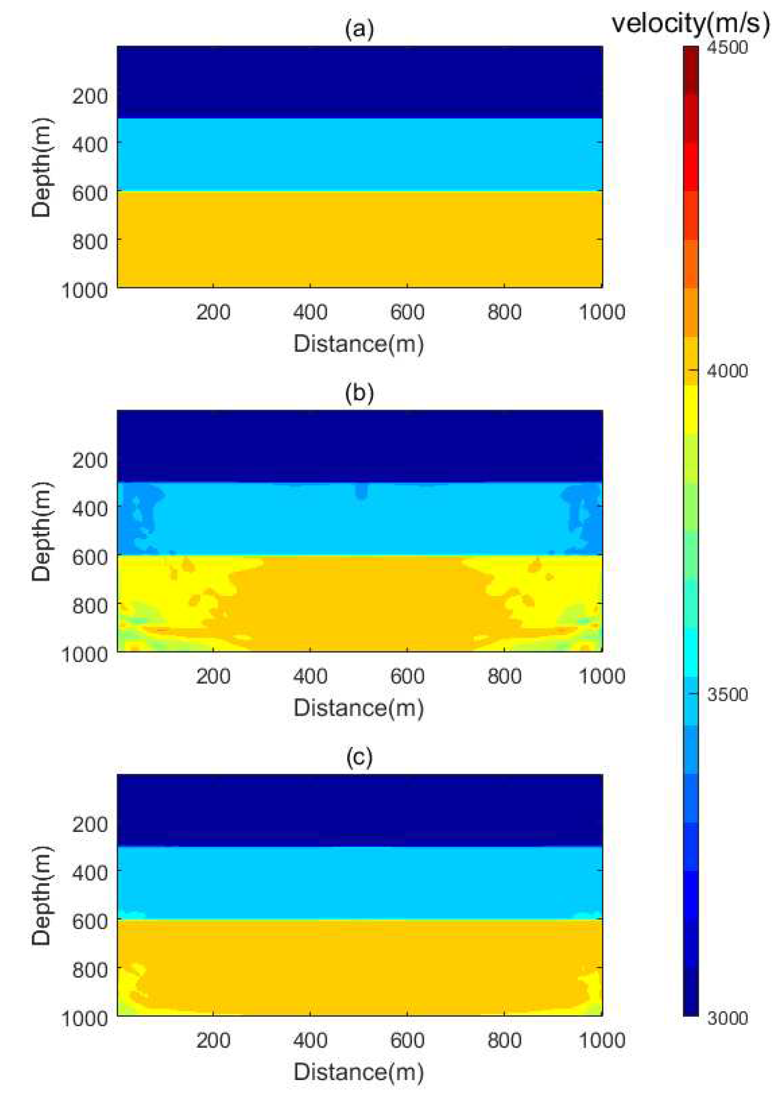
In order to validate the efficacy of the Step-by-Step Inversion Algorithm, a Homogeneous Layer Model was constructed. In this model, the velocities from the shallow to deep regions are set as [3, 3.5, 4] km/s. Synthetic datasets were computed through forward propagation using a Vertical Seismic Profile (VSP) observation system. The initial model has velocities set as [3, 3.4, 3.9] km/s from shallow to deep regions, simulating a scenario where the initial model is relatively accurate. The inversion was performed using the Adam optimization algorithm, with identical parameter settings for all tests. The Homogeneous Layer Model and its inversion results are depicted in
Figure 7.
As can be seen from
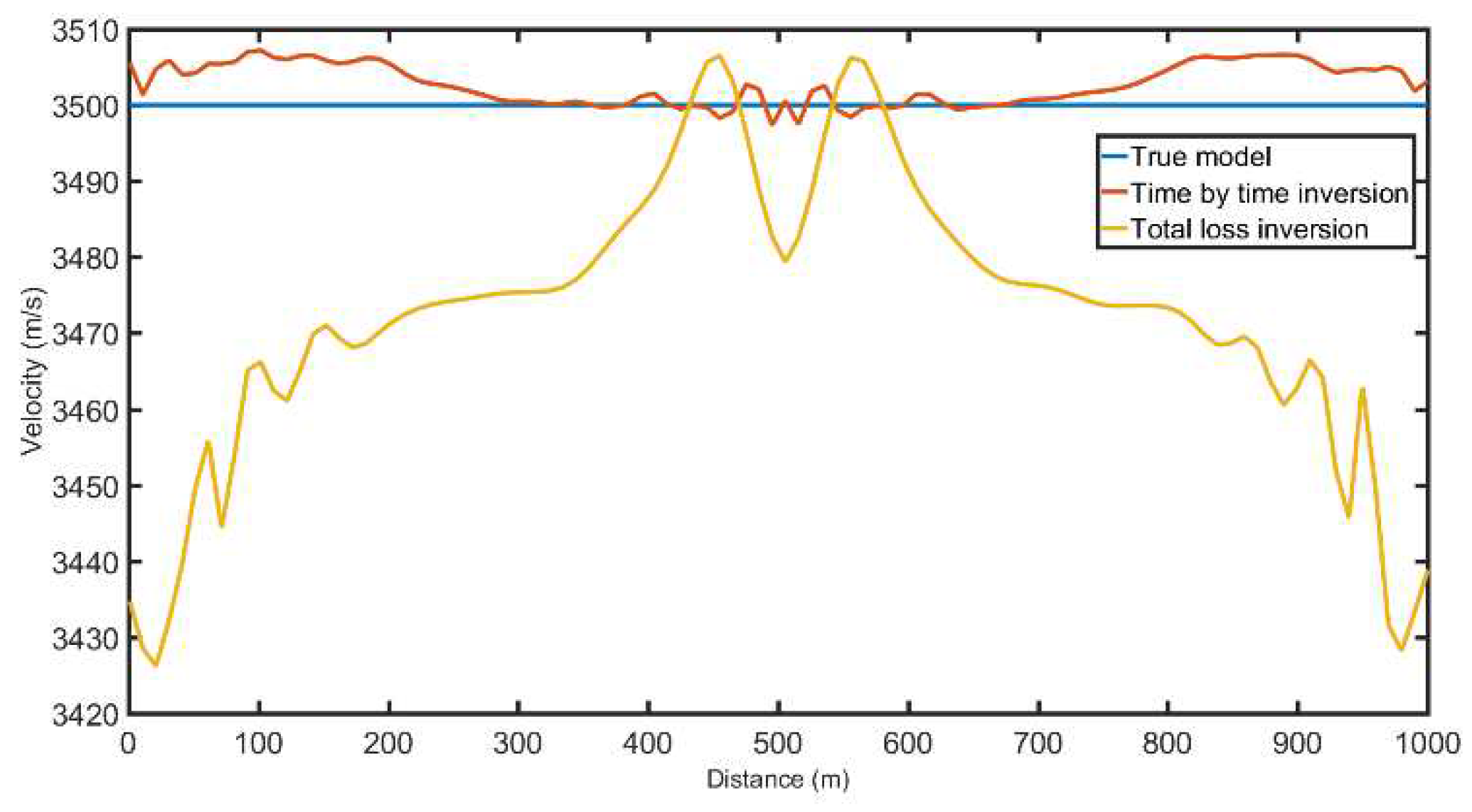
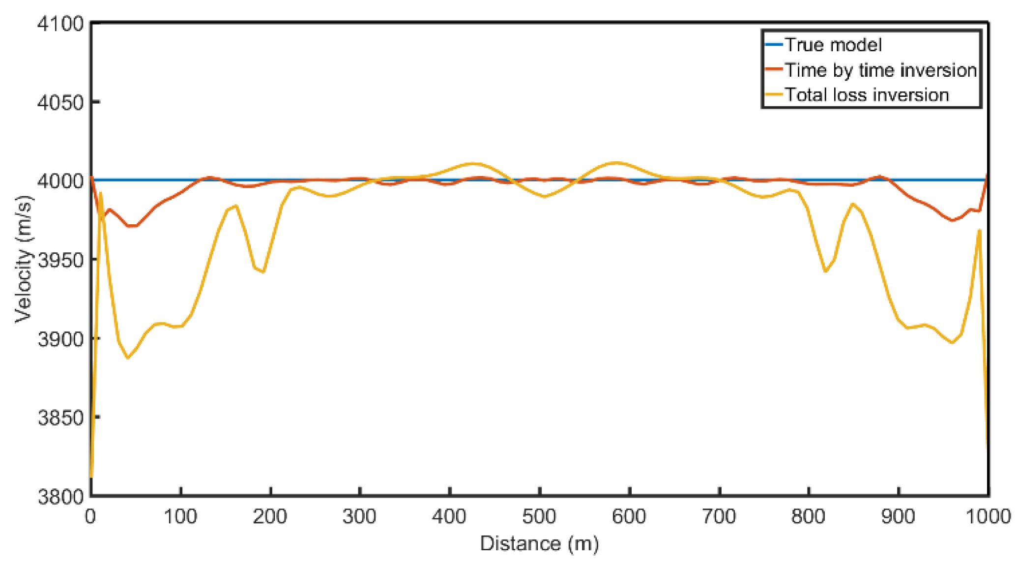
Figure 7, the Step-by-Step Inversion Algorithm yields smoother results both in shallow and deep areas, especially near the source points close to the surface and the lateral regions. Slices were taken at depths of 500m and 800m for velocity profile comparisons, with the results shown in
Figure 8 and
Figure 9 respectively.
It can be deduced from
Figure 8 and
Figure 9 that, in terms of inversion accuracy, the Step-by-Step Inversion generally achieves higher accuracy compared to the Sum-of-Losses Inversion. The inversion results are closer to the true model. Moreover, by employing a time-stepped inversion, which takes into account the propagation of waves, the accuracy of the preceding wavefield is ensured. This, in turn, leads to more precise calculations in subsequent wavefield propagations, manifesting in the inversion results as more accurate representations on the lateral sides and deeper regions of the model.
3.2. Sloping Layer Model
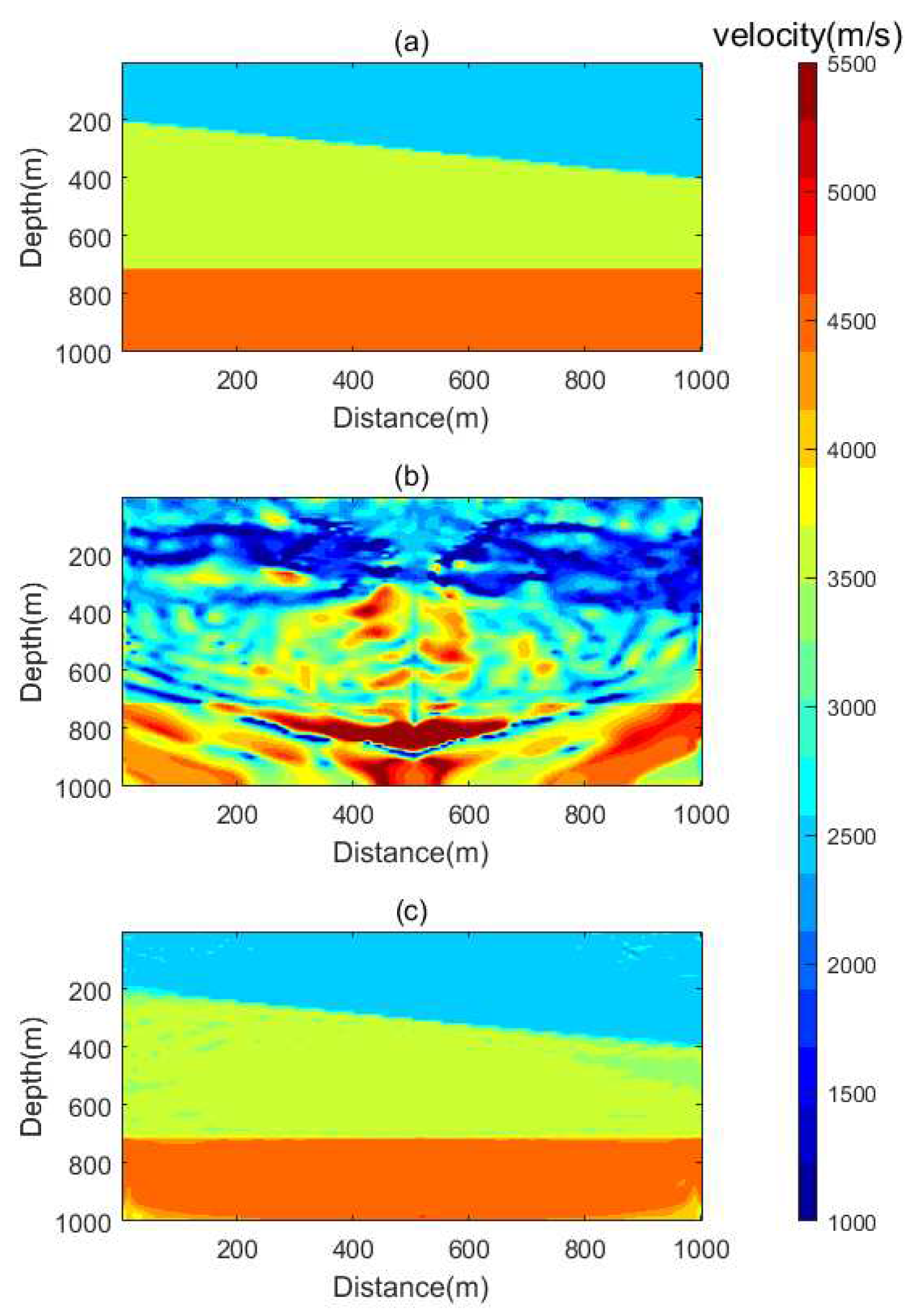
To evaluate the performance of the Step-by-Step Inversion Algorithm in inclined geological structures, as well as its weak dependence on the initial model, a sloping layer model was constructed. In this second model, the velocities increase from the shallow to deeper layers, following [2.5, 3.5, 4.5] km/s respectively. The synthetic dataset was computed using a VSP (Vertical Seismic Profile) observation system via forward modeling. The initial model had velocities [2, 3, 4] km/s, with significant discrepancies between the initial and true models. This was to validate the weak dependency of the Step-by-Step Inversion Algorithm on the initial model, demonstrating that accurate inversion is still achievable despite large errors in the initial model. The inversion employed the Adam optimization algorithm with identical parameter settings. The results of the second model and its inversion are shown in
Figure 10.
As can be observed in
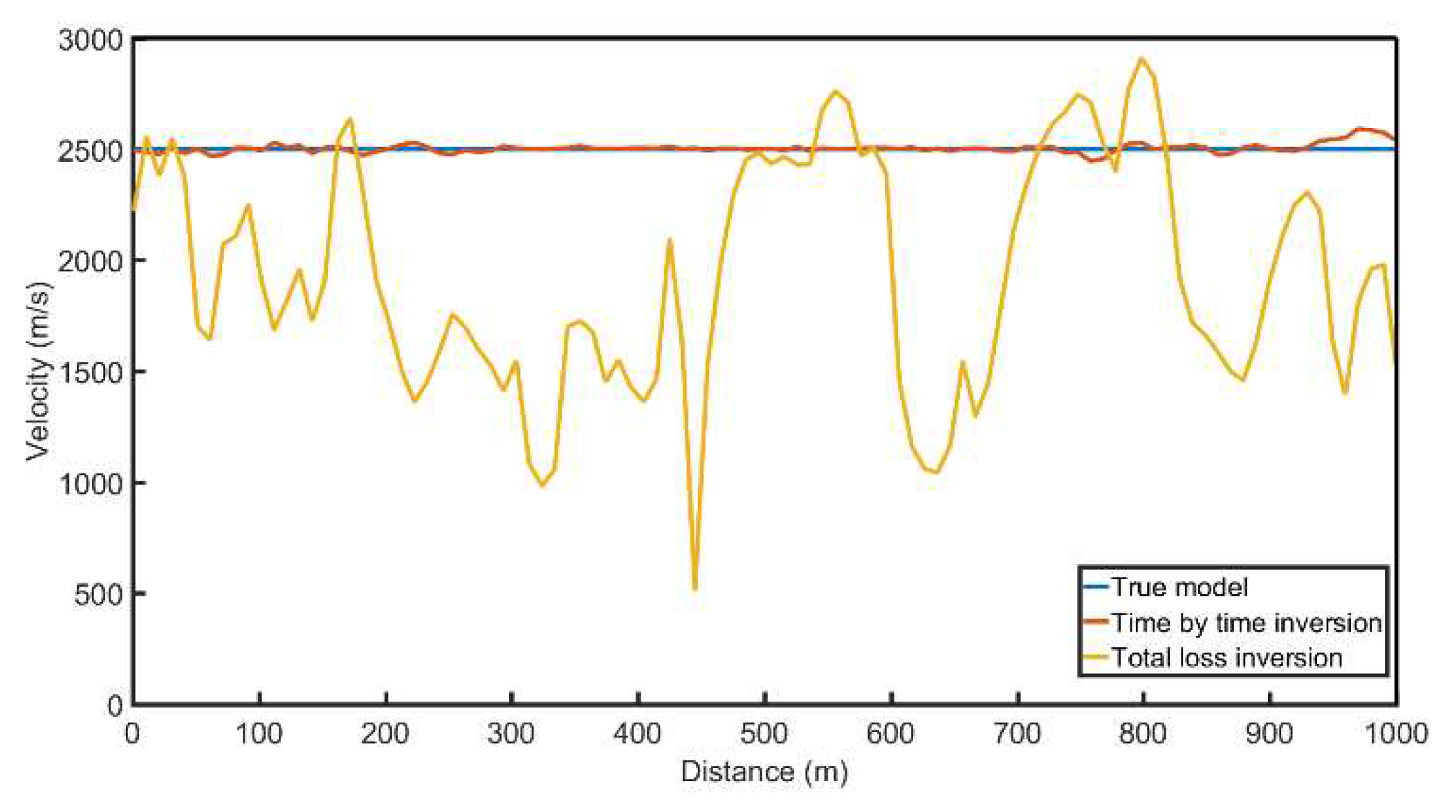
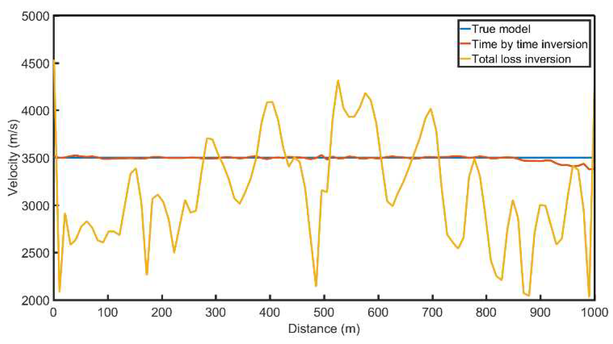
Figure 10, despite the substantial error in the initial model in the context of a sloping layer model, the Step-by-Step Inversion Algorithm exhibited superior performance overall. This suggests that the algorithm has a lower dependency on the initial model and is capable of achieving reasonably accurate inversions even when the initial model has large discrepancies. In contrast, the traditional Sum-of-Losses Inversion performed poorly, indicating a higher dependency on the initial model. Velocity profiles at depths of 150m, 500m, and 800m were selected for comparison and are displayed in
Figure 11,
Figure 12, and
Figure 13 respectively.
Based on the cross-sectional velocity comparison plots, it can be observed that, even with significant errors in the initial model, the Step-by-Step Inversion Algorithm was able to more accurately invert velocities at various depths, including 150m, 500m, and 800m, demonstrating superior precision in the results.
3.3. Marmousi Model
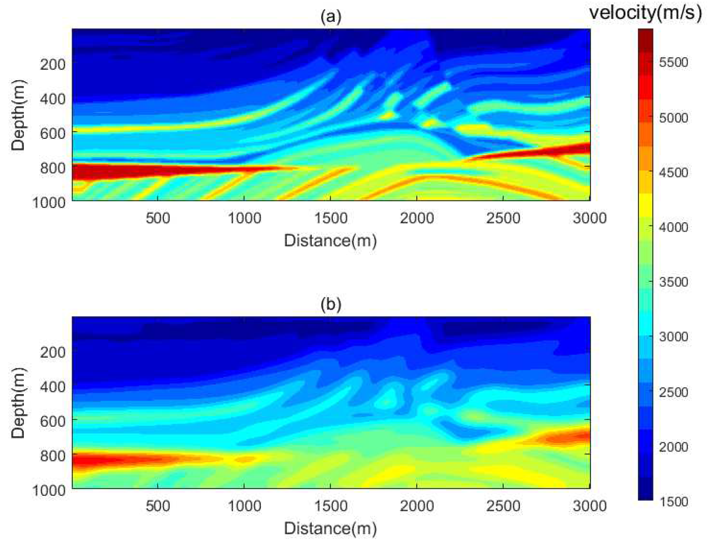
In order to validate the application effect of the algorithm under more complex actual conditions, the Marmousi model was used for experiments. A relatively accurate and smooth velocity model was used as the initial model for inversion. The real model and initial model are shown in
Figure 13. Synthetic data were generated from the real model using the VSP observation system, with the RNN parameters set consistently with the inversion parameters.
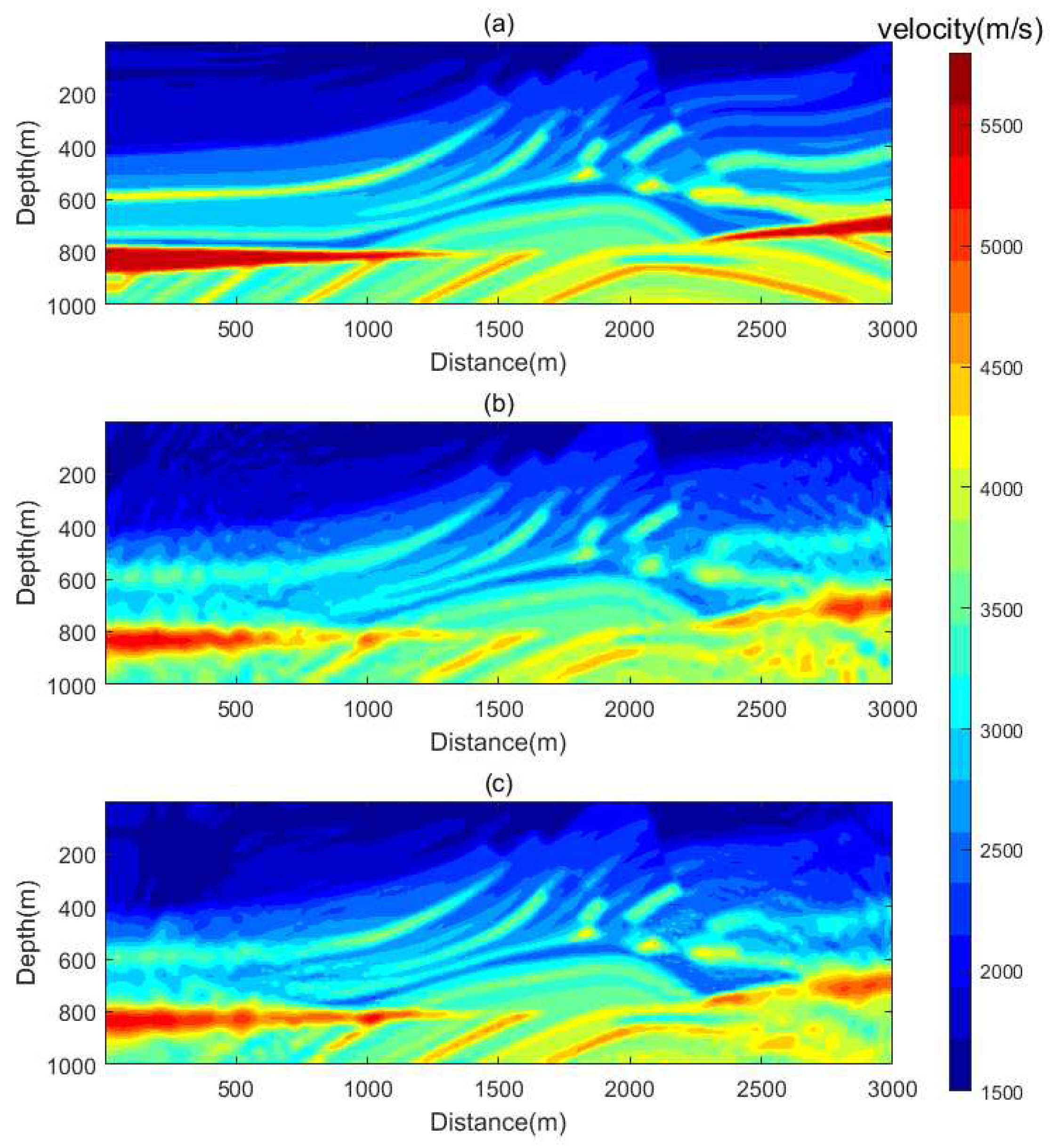
The Marmousi model and inversion results are shown in
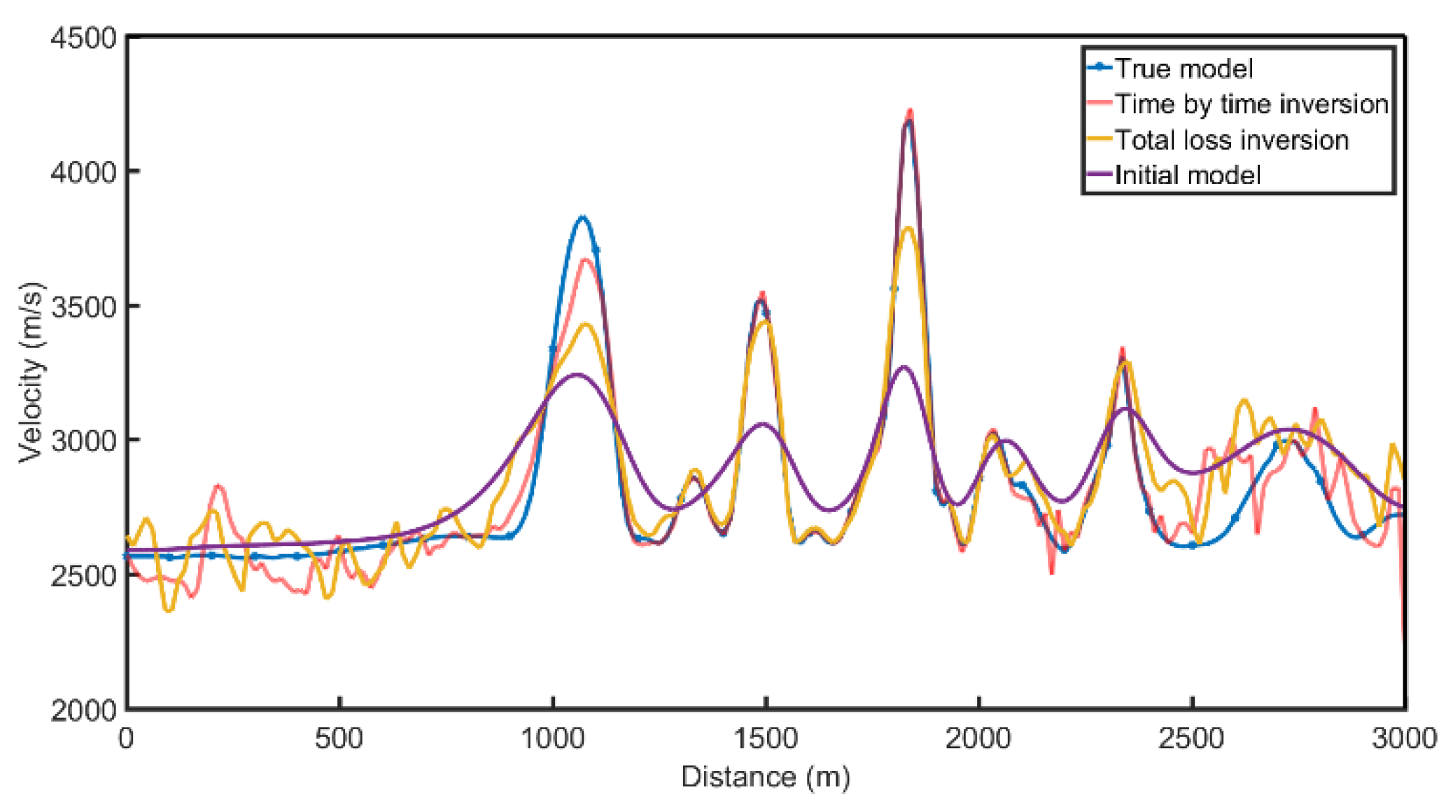
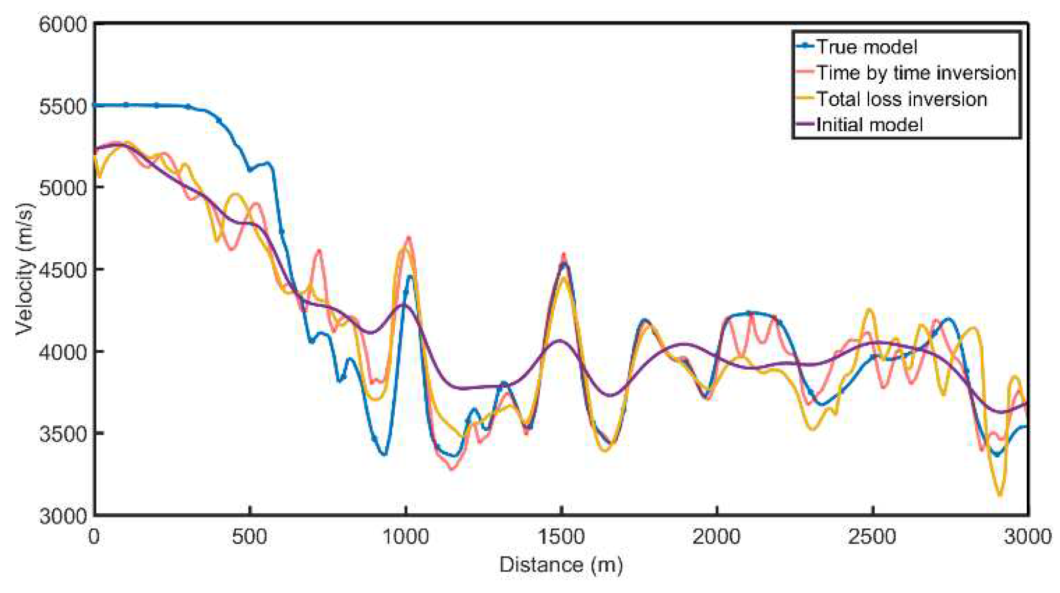
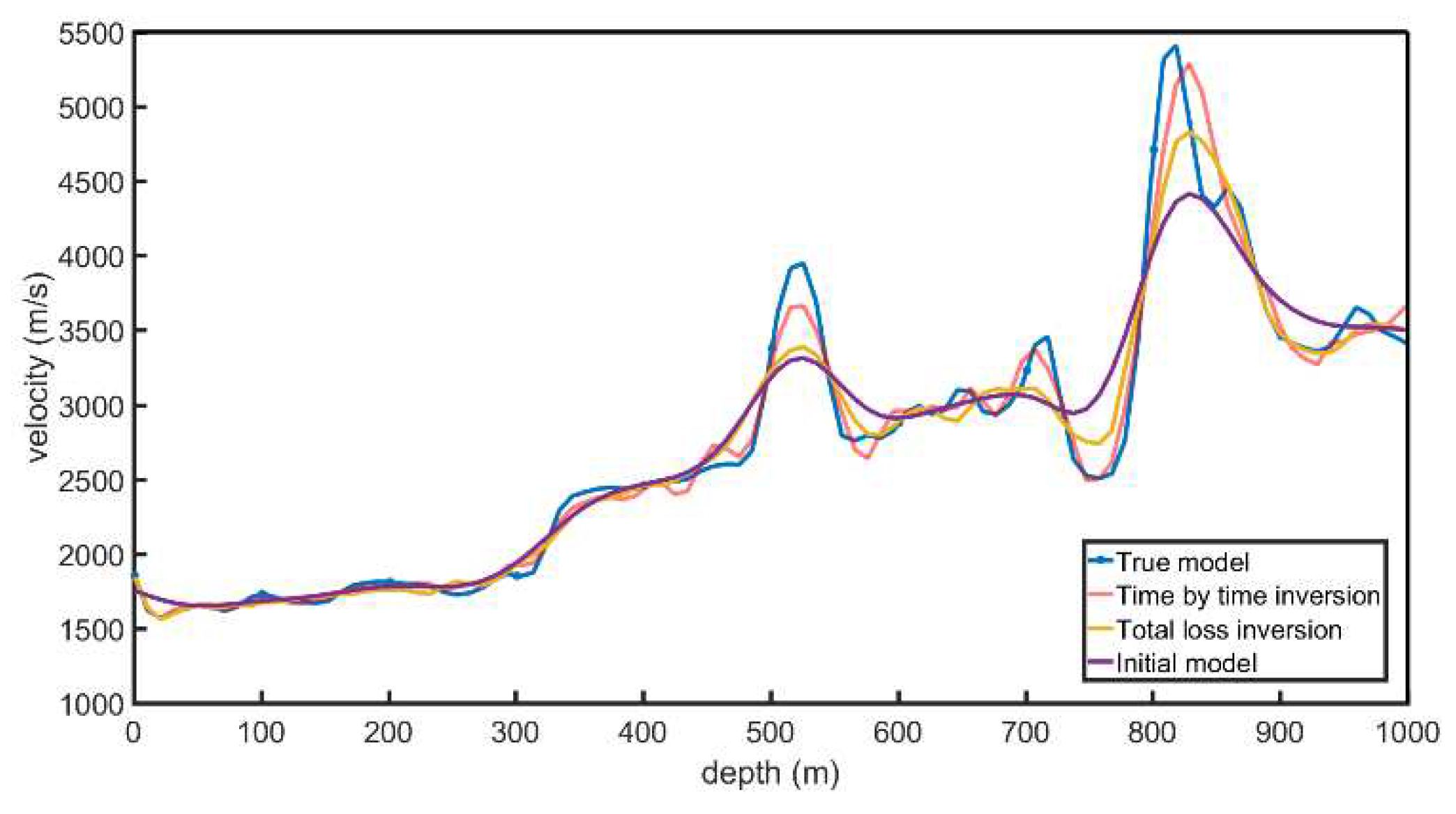
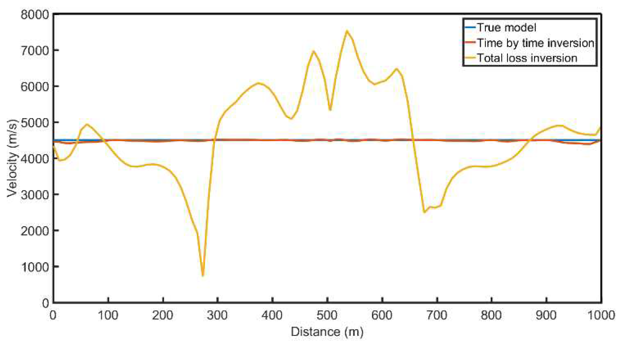
Figure 14. As can be seen from the inversion results, both the overall inversion and time-by-time inversion results are relatively close to the real model. A comparison of horizontal velocity values at depths of 500m and 850m is shown in
Figure 15, and a comparison of depth velocity values at a horizontal distance of 1000m is shown in
Figure 16. From the velocity comparison curve, it can be seen that both the time-by-time inversion and the overall inversion are relatively close to the real model. Moreover, the velocity of the time-by-time inversion results is smoother, with fewer velocity anomalies, making the inversion more stable.
Figure 14.
Marmousi model and initial model. (a)True model. (b)Initial model.
Figure 14.
Marmousi model and initial model. (a)True model. (b)Initial model.
Figure 15.
Marmousi model and inversion results. (a)True model. (b) Total loss inversion (c) Time by time inversion.
Figure 15.
Marmousi model and inversion results. (a)True model. (b) Total loss inversion (c) Time by time inversion.
Figure 16.
Comparison of 500m deep velocity profiles.
Figure 16.
Comparison of 500m deep velocity profiles.
Figure 17.
Comparison of 850m deep velocity profiles.
Figure 17.
Comparison of 850m deep velocity profiles.
Figure 18.
Comparison of 1000m distance velocity profiles.
Figure 18.
Comparison of 1000m distance velocity profiles.
4. Discussion
This paper introduced a Step-by-Step Inversion Algorithm based on a physics-embedded Recurrent Neural Network (RNN). Through the Step-by-Step Inversion Algorithm, the causal information in the temporal evolution of wave equations is mapped to spatial information for velocity model correction. The velocity model is corrected in spatial regions in accordance with the wavefield propagation range. The corrected model then serves as the initial model for subsequent time steps, covering a larger temporal range, which reduces the inversion's dependency on the initial model. Additionally, controlling the correction area results in fewer inversion parameters, effectively reducing the non-uniqueness of inversion solutions within a single time step, and ultimately decreasing the overall non-uniqueness while enhancing the accuracy and stability of the inversion.
5. Patents
This section is not mandatory but may be added if there are patents resulting from the work reported in this manuscript.
Author Contributions
Conceptualization, L.C. and Z.C.; methodology, L.C.; software, Z.C.; validation, Z.C. and Y.C.; formal analysis, L.C.; investigation, L.C..; resources, Z.C.; data curation, Z.C.; writing—original draft preparation, Z.C.; writing—review and editing, L.C.; visualization, L.C.; supervision, L.C.; project administration, L.C; funding acquisition, L.C. All authors have read and agreed to the published version of the manuscript.
Funding
This research was funded by Research on key technology of intelligent geological structure modeling based on tectonic analysis, grant number 41974147.
Data Availability Statement
No new data were created
Acknowledgments
We are grateful to the reviewers for their valuable comments.
Conflicts of Interest
The authors declare no conflict of interest.
References
- Liu Y, He B, Zheng Y. Controlled-order multiple waveform inversion [J]. Geophysics, 2020, 85 (3): R243-R250. [CrossRef]
- Kuang W, Yuan C, Zhang J. Real-time determination of earthquake focal mechanism via deep learning [J]. Nature Communications, 2021, 12: 1432. [CrossRef]
- Zhang J, Zhang H, Chen E, et al. Real-time earthquake monitoring using a search engine method [J]. Nature Communications, 2014, 5 (1): 1-9. [CrossRef]
- Roth, G.; Tarantola, A., Neural Networks and Inversion of Seismic Data. J Geophys Res-Sol Ea 1994, 99 (B4): 6753-6768. [CrossRef]
- Nath, S. K.; Vasu, R. M.; Pandit, M., Wavelet based compression and denoising of optical tomography data. Optics Communications 167 (1-6): 37-46. [CrossRef]
- Kumar, N. S.; Subrata, C.; Kumar, S. S.; Nilanjan, G., Velocity inversion in cross-hole seismic tomography by counter-propagation neural network, genetic algorithm and evolutionary programming techniques. Geophysical Journal International 1999, (1), 1. [CrossRef]
- Yang, F.; Ma, J., Deep-learning inversion: A next-generation seismic velocity model building method. Geophysics 2019, 84 (4). [CrossRef]
- Ren, P., Rao, C., Sun, H., & Liu, Y. (2022). Physics-informed neural network for seismic wave inversion in layered semi-infinite domain. Computational Methods in Applied Mathematics, 22(1), 1-24. [CrossRef]
- Raissi, M., Perdikaris, P., & Karniadakis, G. E. (2019). Physics-informed neural networks: A deep learning framework for solving forward and inverse problems involving nonlinear partial differential equations. Journal of Computational Physics, 378, 686-707. [CrossRef]
- Moseley, B., Nissen-Meyer, T. and Markham, A., 2020. Deep learning for fast simulation of seismic waves in complex media. Solid Earth, 11(4), pp.1527-1549. [CrossRef]
- Moseley, B., Markham, A. and Nissen-Meyer, T., 2020. Solving the wave equation with physics-informed deep learning. arXiv preprint. arXiv:2006.11894.
- Smith, J.D., Azizzadenesheli, K. and Ross, Z.E., 2020. Eikonet: Solving the eikonal equation with deep neural networks. IEEE Transactions on Geoscience and Remote Sensing. [CrossRef]
- Waheed, U.B., Alkhalifah, T., Haghighat, E., Song, C. and Virieux, J., 2021. PINNtomo: Seismic tomography using physics-informed neural networks. arXiv preprint. arXiv:2104.01588.
- Song, C., Alkhalifah, T. and Waheed, U.B., 2021. Solving the frequency-domain acoustic VTI wave equation using physics-informed neural networks. Geophysical Journal International, 225(2), pp.846-859. [CrossRef]
- G. E. Karniadakis, I. G. Kevrekidis, L. Lu, P. Perdikaris, S. Wang, L. Yang, Physics-informed machine learning,Nature Reviews Physics 3 (6) (2021) 422–440. [CrossRef]
- C. Rao, H. Sun, Y. Liu, Physics-informed deep learning for incompressible laminar flows, Theoretical and Applied Mechanics Letters 10 (3) (2020) 207–212. [CrossRef]
- M. Raissi, A. Yazdani, G. E. Karniadakis, Hidden fluid mechanics: Learning velocity and pressure fields from flow visualizations, Science 367 (6481) (2020) 1026–1030. [CrossRef]
- L. Lu, X. Meng, Z. Mao, G. E. Karniadakis, Deepxde: A deep learning library for solving differential equations,SIAM Review 63 (1) (2021) 208–228. [CrossRef]
- E. Haghighat, M. Raissi, A. Moure, H. Gomez, R. Juanes, A physics-informed deep learning framework for inversion and surrogate modeling in solid mechanics, Computer Methods in Applied Mechanics and Engineering 379 (2021) 113741. [CrossRef]
- P. Ren, C. Rao, Y. Liu, Z. Ma, Q. Wang, J.-X. Wang, H. Sun, Physics-informed deep super-resolution for spatiotemporal data, arXiv preprint. arXiv:2208.01462.2022.
- L. Sun, H. Gao, S. Pan, J.-X. Wang, Surrogate modeling for fluid flows based on physics-constrained deep learning without simulation data, Computer Methods in Applied Mechanics and Engineering 361 (2020) 112732. [CrossRef]
- C. Rao, H. Sun, Y. Liu, Physics-informed deep learning for computational elastodynamics without labeled data, Journal of Engineering Mechanics 147 (8) (2021) 04021043. [CrossRef]
- H. Gao, L. Sun, J.-X. Wang, Phygeonet: Physics-informed geometry-adaptive convolutional neural networks for solving parameterized steady-state pdes on irregular domain, Journal of Computational Physics 428 (2021) 110079. [CrossRef]
- P. Ren, C. Rao, Y. Liu, J.-X. Wang, H. Sun, Phycrnet: Physics-informed convolutional-recurrent network for solving spatiotemporal pdes, Computer Methods in Applied Mechanics and Engineering 389 (2022) 114399. [CrossRef]
- H. Gao, M. J. Zahr, J.-X. Wang, Physics-informed graph neural galerkin networks: A unified framework for solving pde-governed forward and inverse problems, Computer Methods in Applied Mechanics and Engineering 390 (2022) 114502. [CrossRef]
- Sun J, Niu Z, Innanen K A,et al.A theory-guided deep learning formulation and optimization of seismic waveform inversion[J].Geophysics, 2019, 85(2):1-63. [CrossRef]
|
Disclaimer/Publisher’s Note: The statements, opinions and data contained in all publications are solely those of the individual author(s) and contributor(s) and not of MDPI and/or the editor(s). MDPI and/or the editor(s) disclaim responsibility for any injury to people or property resulting from any ideas, methods, instructions or products referred to in the content. |
© 2023 by the authors. Licensee MDPI, Basel, Switzerland. This article is an open access article distributed under the terms and conditions of the Creative Commons Attribution (CC BY) license (http://creativecommons.org/licenses/by/4.0/).
