Submitted:
20 November 2023
Posted:
20 November 2023
You are already at the latest version
Abstract
We study the coupling of two topologcal subsystems in distinct topological states, and show that it leads to a precursor behavior of the topological phase transition in the overall system. This behavior is solely determined by the symmetry classes of the subsystem Hamiltonians and coupling terms, and is marked by the persistent existence of subgap states within the bulk energy gap.
By investigating the critical current of Josephson junctions involving topological superconductors, we also illustrate that such subgap states play crucial roles in physical properties of nanoscale devices or materials.
Keywords:
topological insulator
; topological supercondcutors
; zero-energy edge states
; suggap states
1. Introduction
In the more traditional frameworks of the first-order or second-order phase transitions, the states of matter have been classified by symmetry [1]. For topological materials, the states are determined by topology, more specifically, the topological properties of the momentum space that are independent of deformation [2]. By now, there are a plethora of studies on topological states of matter and physical phenomena resulting from the particular topological states [3,4,5]. The signature property of gapped topological materials, i.e., topological insulators, is the so-called zero-energy states, i.e, the states pinned at the zero energy in the middle of the insulating energy gap and localized at the boundary of the material [4]. Ultimately related to the bulk-boundary correspondence of the topological states, the zero-energy states are almost always presumed to be the only subgap states (if any) in the energy spectra of topological insulators (including topological superconductors). That is, it is generally accepted that a topological insulator is characterized by continua of bulk energies and, in the topologically non-trivial phase, the discrete zero-energy states.
In this work, we demonstrate a generic situation where a topological insulator retains subgap states of topological origin other than the zero-energy states. In particular, we show that the interplay between topological states of matter in two coupled topological materials leads to a genuine precursor behavior of the topological phase transition in the overall system. The precursor behavior is governed completely by the symmetry classes of the subsystem Hamiltonians and the coupling term, and are characterized by the persistent presence of subgap states inside the bulk gap. It is crucial to take into account such subgap states in many cases such as the analysis of the critical current of Josephson junctions involving topological superconductors [6,7,8]. The effects of these additional subgap states get more pronounced in nanostructures or low-dimensional materials such as nanowires [9,10,11,12].
2. Model
We consider a coupled system of two bulk-gapped topological subsystems governed by Hamiltonian of the form
where and represent the Hamiltonians of the individual subsystems A and B and describes the coupling between the two subsystems. Each subsystem is assumed to be in a topologically non-trivial phase. Here, we have introduced an explicit parameter to indicate the coupling strength. We will investigate the regime where is turned on from zero to a small but finite value.
Later, we will show that the coupling leads to a generic interplay between topologically distinct states in the two topological materials A and B, which gives rise to persistent subgap states inside the bulk gap. As a brief overview, let us consider a specific case where two subsystems belonging to the BDI symmetry class. When the subsystems are decoupled (), the system belongs to the BDI ⊕ BDI symmetry class. Suppose that both subsystems are in the topological phase. Then, there are edge states associated with each of the subsystems localized at the boundaries. We find that with for weak coupling , there must be genuine subgap states (including the zero-energy states) inside the bulk gap in the total system. This is regardless of whether the total system is in the topological or trivial phase. However, it is instructive to distinguish the two cases. If the total system is in topologically trivial state after turning on , then the subgap states must have finite energy (still inside the bulk gap). In this case, the persistence of the subgap states (well separated from the bulk spectrum) is guaranteed energetically because the weak coupling cannot lift the degenerate states from the subsystems into the bulk continuum with a finite gap. On the other hand, if the total system is in the topological phase, then the subgap states are at the zero energy. Obviously, in this case, they are protected for the topological reasons. In both cases, unless is too large compared with the bulk-energy gap, the subgap states are localized at the boundaries of the system.
2.1. Nanowire as an independent two-band model
In many physical systems, the interplay mentioned above is not immediately apparent. The most prominent example is the nanowire with spin-orbit coupling in proximity to a superconductor and in an external magnetic field as shown in Figure 1 (a). This system is widely recognized as a physical realization of the theoretical model of Kitaev chain, and is known to demonstrate the topological phase transition and associated Majorana edge states predicted in the Kitaev chain [13,14,15]. Throughout this work, we will argue that in fact, the nanowire system involves two topological subsystems (more precisely, two bands in topologically non-trivial phase as elaborated below) and the interplay between them gives rise to a precursor behavior, which has been widely ignored so far, before the topological phase transition.
Here, we briefly review a common picture where the two uncoupled bands in the nanowire system leads to the topological phase transition predicted in the Kitaev chain. Later, we will point out that the residual coupling between the two subsystems plays an important role. The tight-binding Hamiltonian for the system in the momentum space representation reads
with
where
is the single-particle Rashba Hamiltonian and
is the spinor field in the Nambu notation, is the chemical potential of the system, is the Rashba type spin-orbit coupling along y-direction, is the Zeeman field along x-direction, and is the proximity-induced superconducting pairing potential. Without loss of generality, all the parameters are assumed to be positive (with proper choice of gauge if necessary). Band width and chemical potential are typically the largest energy scales in this system, and accordingly, we will assume that both are much larger than both the spin-orbit coupling and superconducting pairing potential ().
As well known [14], the above system exhibits a topological phase transition (TPT) at the critical Zeeman field For Zeeman field greater than , the system is in a topological regime hosting a pair of Majoranas with one Majorana at each end. We call this the ‘main’ topological phase transition to distinguish it from similar transitions in individual subsystems.
The typical picture describing the main topological phase transition starts with identifying two bands. The single-particle Rashba Hamiltonian in Equation (4) gives rise to the two momentum-locked spin bands due to the spin-orbit coupling, i.e.,
where the dispersions are given by
The two electron operators on the two bands ± are related to the bare electron operators via the following unitary transformation
where is the angle between the directions of the Zeeman field and the effective magnetic field that electron with momentum k feels, i.e., see the blue arrows in Figure 1 (b). Their typical dispersion relations are as shown in Figure 1 (b). In these bands, the spin quantization axes are oriented parallel and anti-parallel, respectively, to the effective magnetic field consisting of the external Zeeman field in the x-direction and the momentum-dependent spin-orbit field in the y-direction.
Due to the locking of spin to momentum, mathematically, each of the above two bands can be regarded as describing a spinless fermion. Therefore, turning on the proximity-induced superconducting pairing potential leads effectively to a p-wave pairing within each band. Overall, the bulk Hamiltonian for the nanowire in Equation (2) can be effectively described by
with
where is the strength of the p-wave pairing potentials within individual bands ±, and we have introduced new spinor fields
In this simplified picture, the two bands may be in the topological or trivial phase separately, depending on the values of the chemical potential and the external Zeeman splitting . For example, if (with ), then both bands cross the Fermi level and would be in the topologically non-trivial phase, leading to two Majorana edge states (from respective bands) at each end of the nanowire. Since two Majoranas occupying the same location merge into one Dirac fermion, the topological state of the nanowire in this case is trivial. On the other hand, if then the upper band is off the Fermi level while the lower band remains crossing the Fermi level, leaving one Majorana edge state at each end, and hence the nanowire is in the topologically non-trivial phase. This explains the main topological phase transition at .
In reality, however, the two bands are coupled with each other and cannot be treated separately as in the above argument.
2.2. Nanowire as a coupled two-band model
The coupling between the two momentum-locked spin bands arises for two different reasons. One is the bulk effect. Note that due to the external Zeeman field, the spin quantization axes for opposite momenta are not exactly opposite. Considering that superconducting pairing occurs between electrons with opposite spins and momenta, this leads to off-diagonal components of the pairing in the momentum-locked spin basis. More specifically, the paring potential can be divided into two parts, the intra-band pairing, , already seen in Equation (10) and inter-band pairing, depending on whether it is diagonal or off-diagonal; see Figure 2 (a). This leads to a more complete description of the nanowire Hamiltonian in Equation (2) in the form
where describe the two bands ± as defined in Equation (10) and
is responsible for the inter-band coupling.
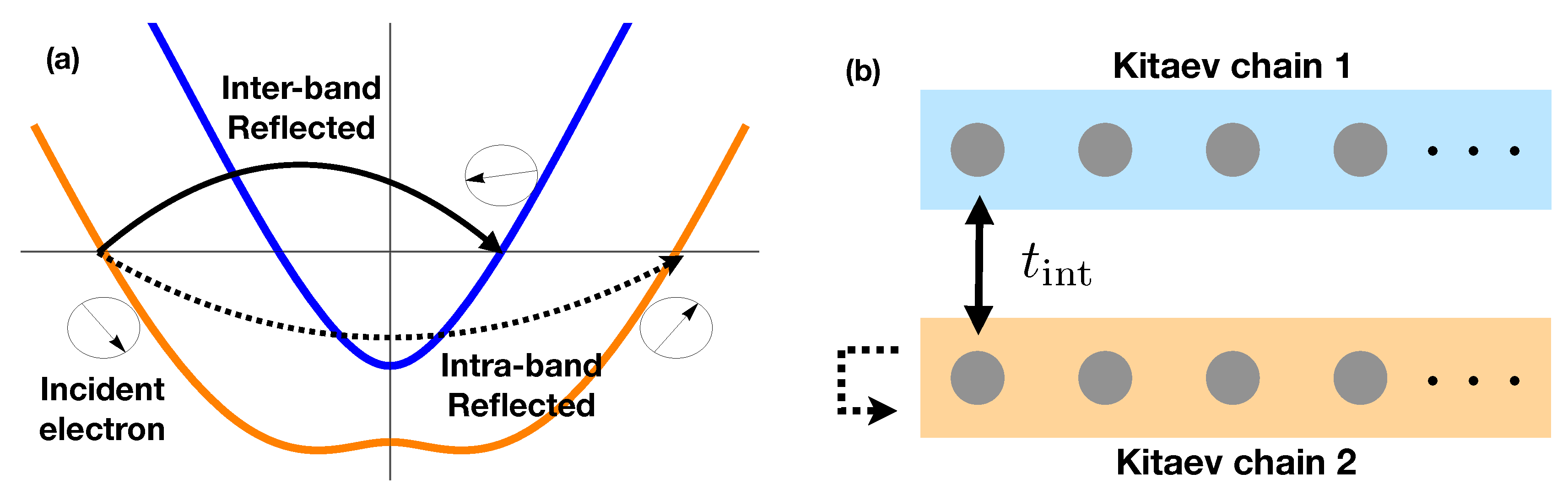
The other source of the coupling between two bands is the reflection at the boundary of the nanowire. This coupling originates in the spin mismatch between left-going and right-going electrons in the same band. When a left-going electron in the lower band, for example, reflects at the boundary, it cannot be reflected exclusively into the lower band due to the spin conservation (see Figure 3 (a)). There should be a reflected wave in the upper band as well. This can be clearly seen when we express the annihilation operators, and , for electrons with spin up and down, respectively, in terms of the operators for electrons with the momentum-locked spins ±,
where
with unitary matrix defined in Equation (8). Since the spin rotation matrix depends on k, is not diagonal in general. This means that even a simple boundary condition in position space, such as an open or hard boundary, induces reflections from one band to the other.
Figure 2.
(color online) Relation between the nanowire and coupled Kitaev chains. (a) Dispersion relation without superconductivity. Superconducting pairing is represented as arrows. Curved red arrows indicate the pairing within the same band. The black arrow is for the pairing between the different bands. (b) Two coupled Kitaev chains as a model for nanowire. The blue(orange) bar with an illustration of a tight-binding model represents a Kitaev chain that corresponds to the upper(lower) band of the nanowire and the intra-band pairing of the band. Black vertical arrows are for the parametric coupling between two Kitaev chains, which corresponds to the inter-band pairing of the nanowire.
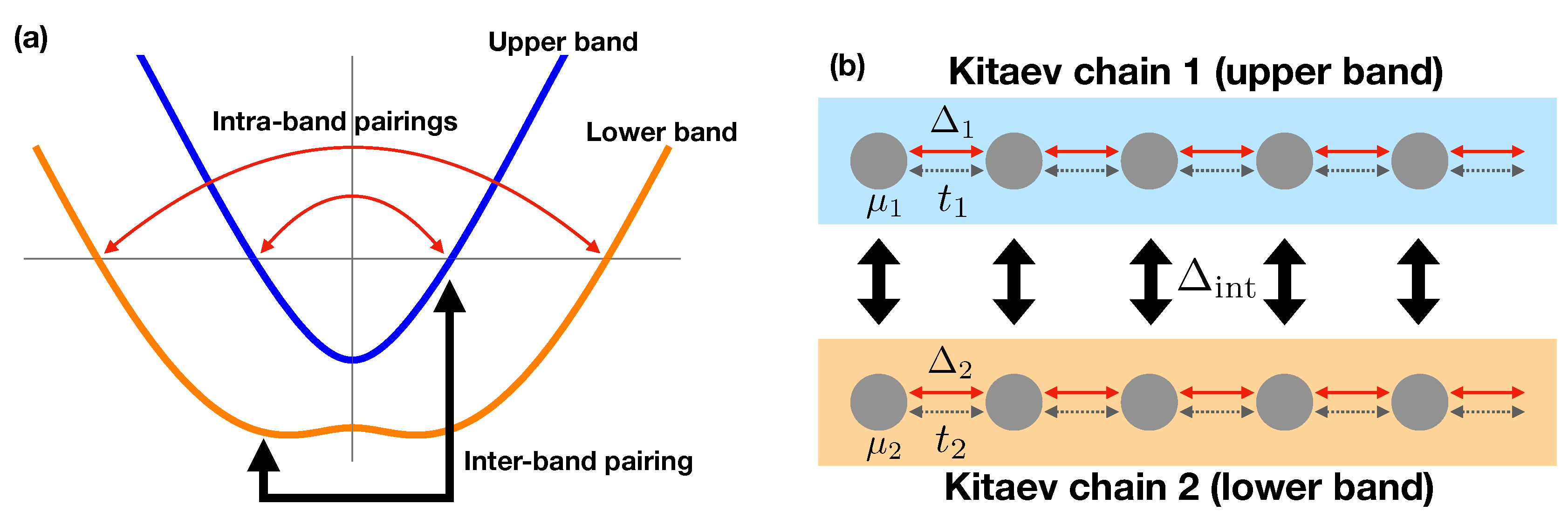
Figure 3.
(color online) (a) Schematic illustration of reflections at the Fermi energy. Spin directions The arrows in black circles represent the spin directions, and the blue and orange curves display the energy dispersions for both bands. The dotted curved arrow is for the intra-band reflection, and the solid curved arrow is for the inter-band reflection. (b) The inter-band (solid arrow) and intra-band (dotted arrow) reflections in coupled Kitaev chains. In particular, the inter-band reflection is modeled as hopping with amplitude between two chains at a single site near the boundary.
2.3. Coupled Kitaev Chains
Before we discuss the effects of the inter-band coupling on the topological properties of the nanowire system, to avoid the unnecessary complexity and to focus on the main physics, we examine the same effects in a toy model that has the key features of nanowire. Our toy model is composed of two coupled Kitaev chains as schematically depicted in Figure 2 (b) and Figure 3 (b), its Hamiltonian reads as
Here, the isolated upper () and lower () Kitaev chains are described by
where is a fermion creation (annihilation) operator at site x, the hopping amplitude, the pairing potential, and the chemical potential on chain . We set , such that without any coupling between the chains, both chains are in the topological phase. The term
is responsible for the coupling due to the inter-chain pairing potential [see Figure 2 (b)] whereas the term
describes the reflection from one chain to the other at the boundaries () with reflection amplitude [see Figure 3 (b)].
We take the toy model in Equation (16) as a simplified model of realistic nanowires, and the connection between the two models is already clear from corresponding and resembling terms. However, some of the simplifications is worth mentioning. In the nanowire model, the inter-band pairing, in Equation (13), depends on momentum k. However, the complex phase (including signs) does not change as the momentum k varies because . Therefore, we take the inter-chain coupling constant in k as shown in Figure 2 (b). The relative phases of all three pairing potentials, , and cannot be eliminated by a U(1) gauge transformation, but the relative phases of any two of them can be fixed by choosing a proper gauge. Throughout the work, we fix the complex phases of intra-chain pairing and to and 0, respectively, i.e., and .
3. Persistent subgap states
3.1. Two Coupled Kitaev Chains
As the first examples of physical implications of the interplay of two subsystems in topologically distinct states, we first investigate the toy model of coupled Kitaev chains described in Equation (16). As we assumed in Section 2.3, both Kitaev chains are in the topological phase when they are decoupled, and each chain hosts one Majorana bound state at its each end. It will be instructive to regard the inter-chain pairing and hopping as independent parameters. When we eventually compare this toy model to the nanowire model, the inter-chain pairing must be real-valued. We lift this constraint and allow it to take arbitrary complex phase to investigate a broader impacts of coupling on the symmetry classes of the total system.
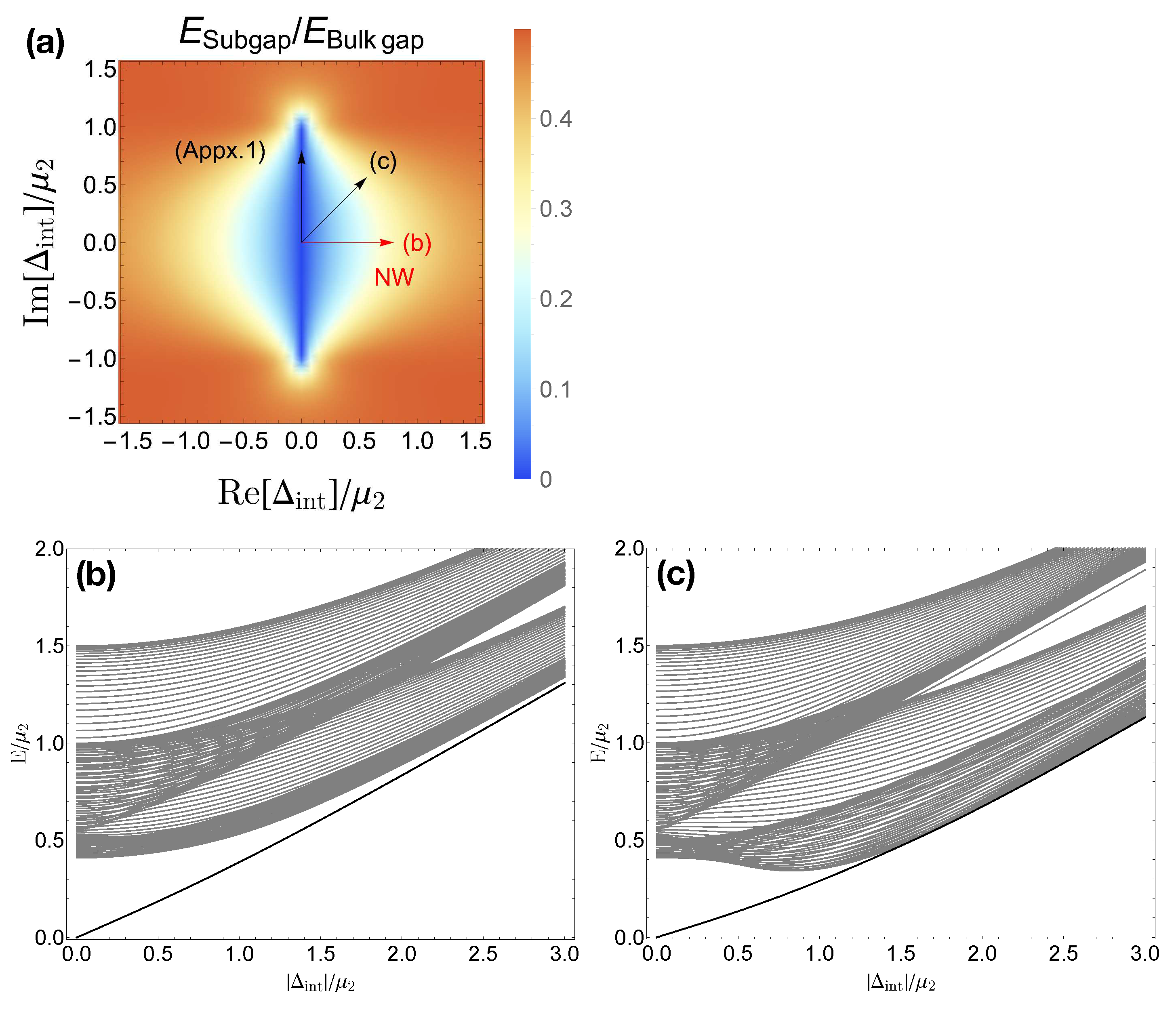
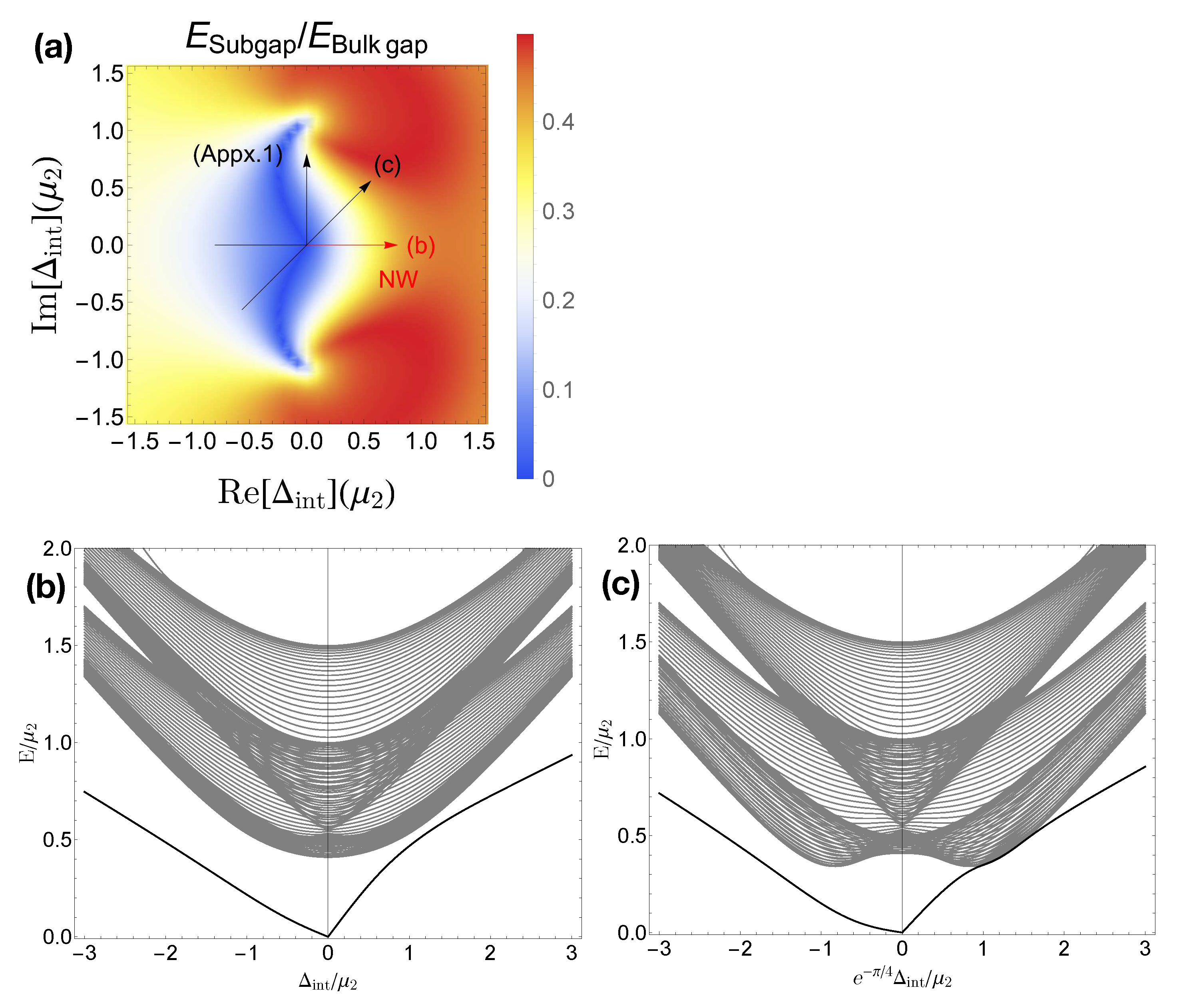
First, let us turn on only the inter-chain pairing; and . The ratio between bulk gap energy and subgap energy is shown in Figure 4 (a). When the coupling is zero, , the two Majoranas at each end exist at zero energy(by ignoring the small coupling proportional to ), such that the ratio between the bulk gap and subgap energy, is zero. As we turn on the coupling, the energy starts to change. Note that if the inter-chain pairing can have an arbitrary complex phase, the symmetry class of the coupled system is D with its allowed topological invariant . It means that at least one of the two Majorana bound states at one end should disappear. However, as it is well known, a single Majorana bound state cannot disappear through the interaction with bulk states because of the finite bulk gap energy. Therefore, the system should be in a topologically trivial phase, such that the two Majorana bound states are to interact with each other and be merged into a Dirac state with its energy within the bulk gap, which is shown in Figure 4 (a). The nanowire analogy result is shown in Figure 4 (b). As the parameter, , changes along the positive real axis, we have nonzero subgap state energy within the bulk gap.
Note that an accidental degeneracy could arise, i.e., an accidental symmetry may prevent the two Majoranas from interacting with each other. Under the exclusion of the inter-band hopping, it happens when the inter-chain pairing is pure imaginary, . In this case, the subgap states are fixed at zero energy until the coupling becomes sufficiently large to close the band gap, and the subgap states disappear through the band touching. The detailed discussion of this regime will be presented in Appendix A with relevant figures in Figure A1.
Figure 4.
(color online) Energy profiles of the two coupled Kitaev chains model as a function of inter-chain parametric pairing, . Inter-chain hopping is turned off. (a) Ratio between the subgap-state energy and bulk gap energy. The subgap-state energy is measured from the Fermi level, such that the ratio converges to when the subgap energy is merged into bulk. Inset arrows (Appx.1) is for the appendix. (b,c) Energy levels along the arrows in panel (a), i.e. complex phase of the pairing is fixed to , and in (b) and (c), respectively. The pure real corresponds to the nanowire model. Only the positive energy levels are shown as the system has particle-hole symmetry. Parameters: The number of sites for a chains , on-site energy , (unit energy scale), intra-chain pairings , hoppings .
Second, we set the parametric pairing equal to zero and consider the inter-chain reflection as the only coupling between the chains. The results are presented in Figure 5. Unlike the varying case, the inter-chain hopping exists only at the boundaries, such that the bulk band does not show any significant changes. Besides this difference, the overall behavior of the energy of the subgap state can be seen within the similar context. The set of Hamiltonians with the arbitrary complex number is in the symmetry class D, so the system is in a topologically trivial phase for the same reason as mentioned above. Starting with zero energy states at , we have finite subgap energy well separated from the bulk band.
Finally, in Figure 6, we take both inter-chain pairing and hopping into account simultaneously. We set the pure real inter-chain hopping and vary the pairing with an arbitrary complex phase as we did previously. Unlike the previous results, the interplay between two couplings, and , makes subgap energy now depends on the complex phase of more asymmetrically.
3.2. Nanowire
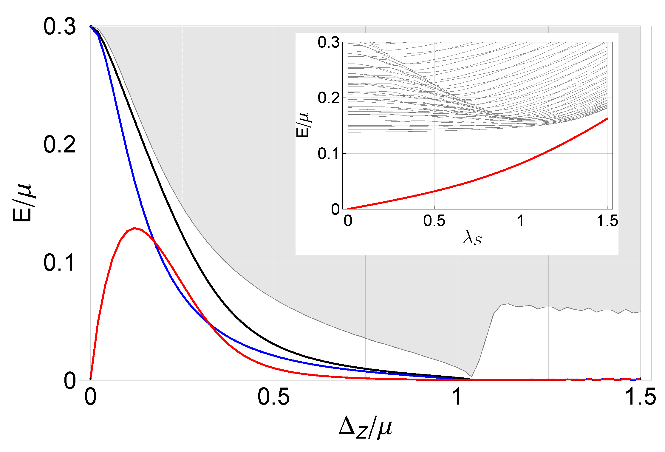
In this section, we will consider a more realistic model, that is, the nanowire. Subgap energy and the bulk band of the nanowire system as a function of the Zeeman field are given in Figure 7. As mentioned earlier in Section 2.1, when the Zeeman field is larger than the critical field , the system is in the topological phase. The Majorana bound states exist at the zero energy (ignoring exponentially small coupling between Majorana states at opposite edges). With the Zeeman field smaller than the critical field, we find the subgap state(black curve) originates in the interplay of two Majoranas from upper and lower bands, respectively.
Before we discuss the result, let us consider inter-band pairing and reflection separately, as we did in the previous section.
First, the case with truncated inter-band reflection is following. To eliminate the inter-band reflection, we express the Hamiltonian in momentum space using the momentum-locked spin basis depicted in Equation (11). Then, we take the inverse Fourier transformation, such that the position space operator, , will be written as Equation (14). Because of the non-local nature of this basis, the open boundary can no longer be written in a simple form. Instead of using the usual open boundary condition, as we are interested in ignoring the inter-band reflection, we impose a new open boundary condition directly on this basis. In this way, we obtain the red curve in Figure 7, the subgap state energy without the inter-band reflection. When the Zeeman field is zero, there will be no inter-band pairing due to the exact spin matching between opposite spin electrons with the opposite momentum. So, the subgap energy converges to zero. As the Zeeman field increases, the inter-band pairing also increases, such that we have the finite subgap state energy. After the peak near , it is hard to make a qualitative description.
To verify that the inter-band reflection is properly truncated and show the finite subgap energy originates in the inter-band pairing, we calculate energy levels as a function , where for a modifier in front of the inter-band pairing, for all k. See the inset of Figure 7. As the parameter goes to zero, there will be no coupling at all between the two bands, such that the subgap state energy goes to zero as we have seen in the two coupled Kitaev chains model.
Second, let us describe the case that the inter-band reflection is the only coupling between two bands. The result is obtained by imposing the usual open boundary condition to the bulk model with . See the blue curve in Figure 7 where the subgap energy solely comes from the inter-band reflection. When the Zeeman field vanishes, the direction of the effective magnetic field is simply determined by the Rashba-field. As the direction of the Rashba field is opposite for electrons with opposite momentum, there will be total reflection between two bands so that we have large inter-band coupling with large subgap energy merging into the bulk.
In summary, we find the subgap energy of the nanowire in the parameter regime before the topological phase transition occurs. Together with the finite subgap energy, we find the origins of the subgap energy, inter-band pairing and reflection. The effect of the inter-band pairing is studied with modified pairing , while the effect of inter-band reflection is discussed qualitatively.
Figure 7.
(color online) Subgap energy with different conditions and bulk energy levels of the nanowire as a function of the Zeeman field is given. Gray area indicate bulk state energy, and black line is for the subgap state energy. The red line is the subgap energy when inter-band reflection is forbidden. The blue line is for the subgap energy without the inter-band pairing, i.e. the inter-band reflection is the only coupling between bands. The vertical dashed line is for the inset figure. We used tight binding model with , and . The critical Zeeman field is approximately (Inset) Energy level versus modified inter-band pairing strength for all k. The inter-band reflection is turned off. The vertical dashed line indicate . Parameters are , and .
4. Critical current
In this section, we now present the physical implication of the subgap states discussed above on the critical current of the nanowire junction.
We calculate the zero-bias critical current by using linear response theory for the nanowire connected to a normal superconductor or a topological superconductor as a function of the Zeeman field and temperature. Both the normal and topological superconductors, as well as the nanowire, are expressed by tight-binding models Equation (2) with appropriate parameters. We assumed a tunnel junction, expressed by the tunneling Hamiltonian,
where is an electron creation operator on the junction side with its and spin and t is a tunneling amplitude. Without loss of generality, we set R to be the nanowire and L to be a normal superconductor or a topological superconductor.
To find the contribution of the subgap state to the critical current, we divide the critical current into two parts, localized states contribution and the rest. The meaning of these division will be presented below.
For the normal superconductor-nanowire junction(NS-NW), the normal superconductor does not have any localized state. Therefore, as shown in Figure 8, the critical current can be divided into two terms, bulk-bulk and localized-bulk. We find a finite contribution to critical current from the localized state. Note that when the Zeeman field exceeds the critical value, i.e., when the nanowire is in the topological phase, there is no supercurrent through the localized state (Majorana bound state) [16]. The finite contribution of the localized state can be found only in the topologically trivial regime.
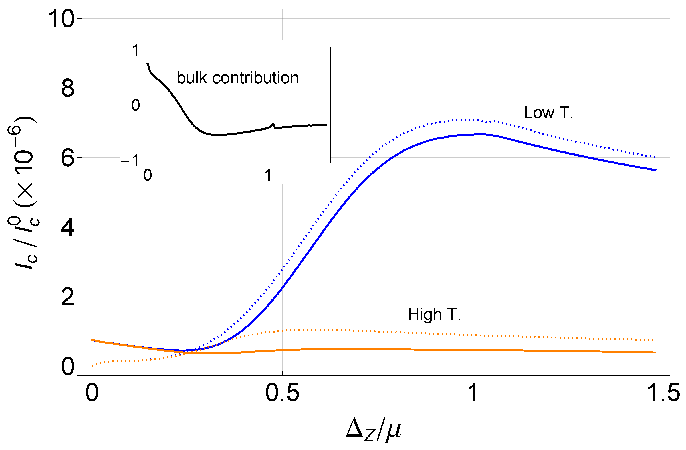
For the topological superconductor-nanowire junction(TS-NW), we find that most supercurrent flow through the localized states (see Figure 9). Interestingly, even when the nanowire is in the trivial phase one cannot ignore the subgap state; it has a finite contribution to the critical current. Unlike the NS-NW junction, the temperature severely affect the critical current since the majority of critical current flows through the lowest energy states, namely, the subgap state in the nanowire and Majorana bound state in the topological superconductor.
Figure 8.
(color online) Zero bias critical current , where is the critical current in the short-junction limit, between a normal superconductor and the nanowire obtained by the tight-binding model is presented. Parameters are for the normal superconductor and for the nanowire. Tunneling amplitude is . Temperatures are . (Inset) Critical current through the bulk states of the normal superconductor and the nanowire(Solid line) and through the subgap state at the nanowire and bulk states of the normal superconductor(Dashed line) with the low temperature is given. Axis units are the same as used in the main plot.
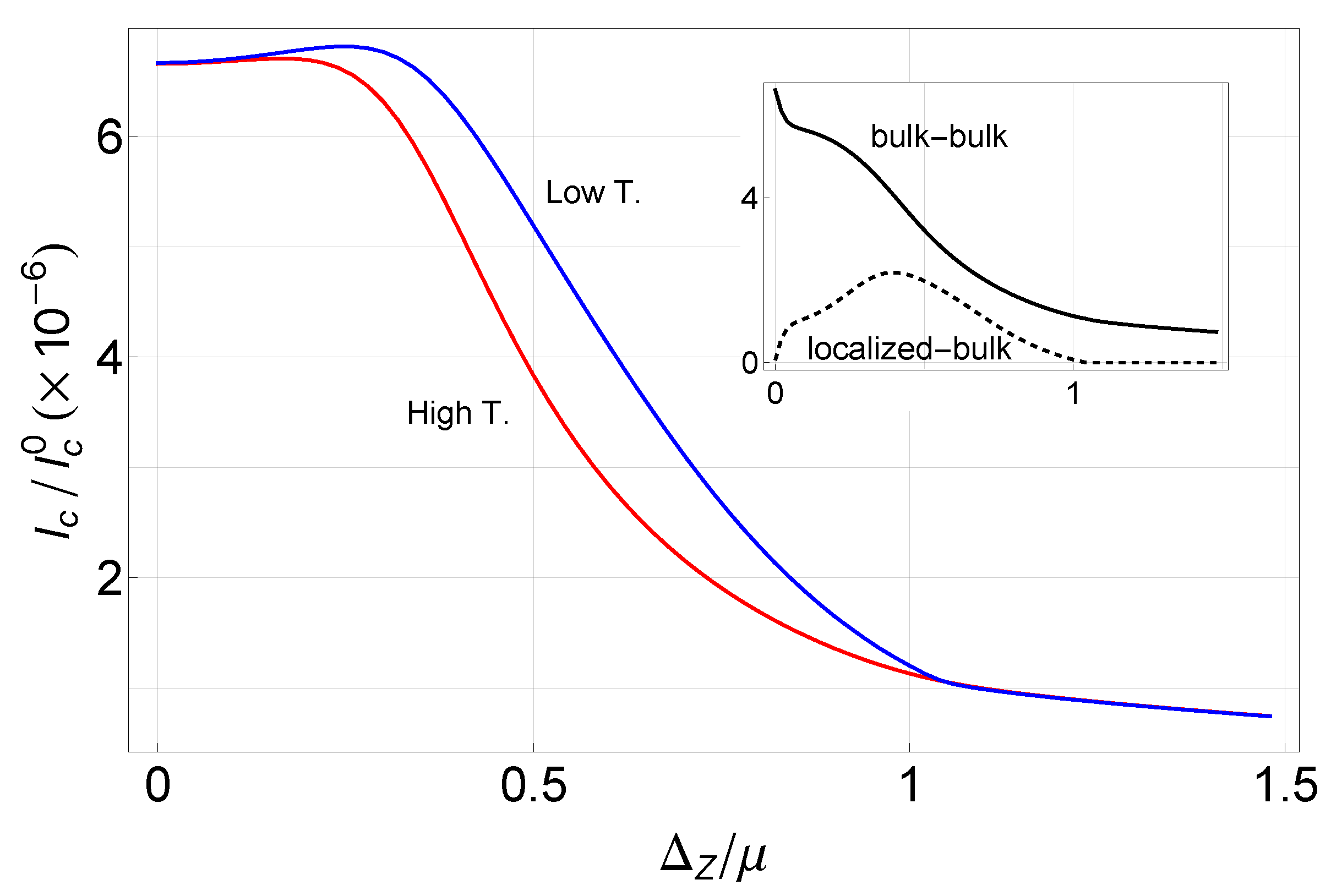
Figure 9.
(color online) Zero bias critical current between a topological superconductor and the nanowire obtained by the tight-binding model is given. Solid lines indicate critical current. Dotted lines are for current through the localized states. We use topological superconductor parameters, , and the nanowire parameters = . Tunneling amplitude is . Temperatures are . A small kink near the phase transition, , is due to a systematic error, i.e. the localized state and bulk states are not well separated near the point. (Inset) The critical current that bulk states contribute, i.e., bulk states to bulk states and localized states to bulk states.
5. Conclusion
We have examined coupled topological subsystems, each in different topological states of matter, and reveal that this interaction results in a precursor effect during the topological phase transition within the entire system. This effect is entirely governed by the symmetry classes of the subsystem Hamiltonians and the coupling term, and it is characterized by the continuous presence of subgap states within the bulk energy gap.
By analyzing the critical current in Josephson junctions incorporating topological superconductors, we have demonstrated the essential roles these subgap states play in the physical properties of nanostructures and low-dimensional materials.
Author Contributions
Conceptualization, M.-S.C.; methodology, S.H. and M.-S.C.; validation, S.H. and M.-S.C.; formal analysis, S.H. and M.-S.C.; investigation, S.H. and M.-S.C.; data curation, M.-S.C.; writing—original draft preparation, S.H.; writing—review and editing, M.-S.C.; visualization, S.H. and M.-S.C.; supervision, M.-S.C.; project administration, M.-S.C.; funding acquisition, M.-S.C. All authors have read and agreed to the published version of the manuscript.
Funding
This work was supported by the National Research Function (NRF) of Korea (Grant Nos. 2022M3H3A106307411 and 2023R1A2C1005588) and by the Ministry of Education through the BK21 Four program.
Institutional Review Board Statement
Not applicable.
Informed Consent Statement
Not applicable.
Data Availability Statement
All data created are included as figures in this paper.
Acknowledgments
Not applicable.
Conflicts of Interest
The authors declare no conflict of interest.
Appendix A. Accidental symmetry of the two coupled Kitaev chains model
In Section 3.1, we investigatd the effects of inter-chain coupling with arbitrary phase. Here, we will discuss the special case that the inter-chain pairing is pure imaginary. The point is that this constraint on the inter-chain coupling can lead to additional anti-unitary symmetries which affect the topological class of the model. However, such a constraint and result topological class is illusive in the sense that it easily breaks down in realistic situation such as local disorders and next nearest-neighbor (NNN) couplings. On this ground, we emphasize that the classification and corresponding discussions in Section 3.1 are physically valid in general. Nevertheless, we present the analysis of the topological class of this special case to avoid potential confusion when one encounters the similar situation with illusive anti-unitary symmetries.
Recall that the phase of intra-chain pairings are fixed to and without loss of generality; in other words, the phase of the inter-chain pairing is a gauge-fixed quantity.
With the given constraint (and assumption ), the model acquires a time-reversal-like symmetry operation ,
such that the Hamiltonian satisfies
It is stressed that this symmetry operation is not related to the physical time-reversal symmetry. Since we consider the model of coupled Kitaev chains as an analogy to the nanowire model which is composed of electrons, the physical time reversal symmetry operator should satisfy the relation , where for electron number operator. To the contrary, the symmetry operator of our interest here satisfies .
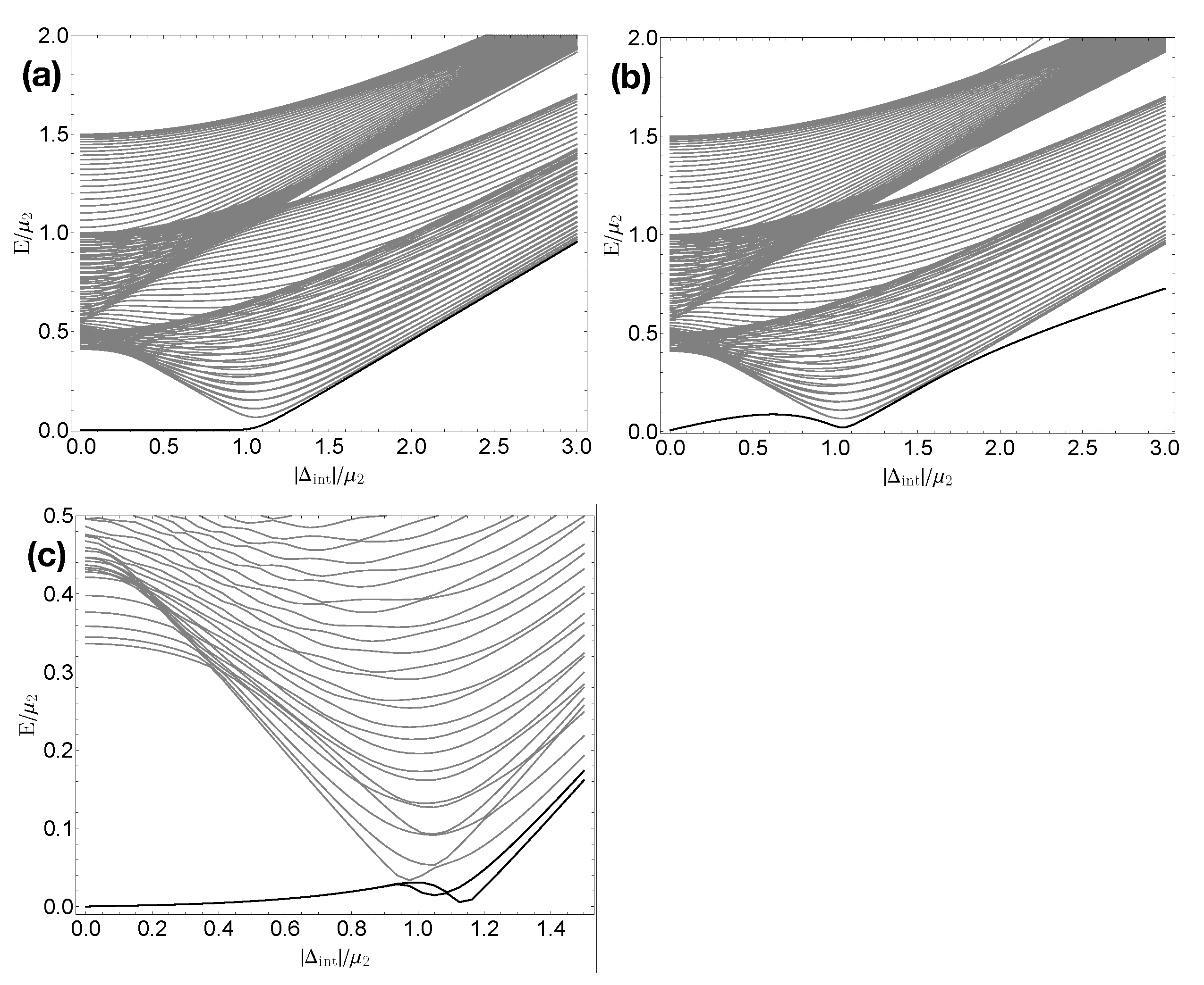
Though the symmetry described by is not a physical time-reversal symmetry, it determines the symmetry class of the Hamiltonian. Together with the particle-hole constraint of the BdG Hamiltonian, the relevant symmetry class of the system is BDI and the relevant topological invariant is the winding number. This winding number captures the number of the chiral Majorana bound states localized at one end; that is, it represents the number of Majorana bound states with different chiralities (i.e., eigenvalues of the chiral operator) at one end. In our case, as briefly mentioned in Section 3.1, if we change the strength of the inter-chain pairing , the two chiral Majoranas at each end remain at zero energy until the gap closes. The winding number is 2 before the gap closes, so the two Majorana bound states on the left end of the chains have chirality while the other two states on the right end have chirality . After the gap closes, the winding number is changed to 0 and there are no Majorana bound states anymore; see Figure A1 (a).
However, unlike the usual unpaired Majorana bound states, the energy of the above states can be easily lifted from zero as the time-reversal-like symmetry can be easily broken if we introduce additional interactions or local disorder. For example, inter-chain hopping terms, , or NNN hopping terms with nonzero complex phase, i.e. , would break the time-reversal-like symmetry, such that the energy of boundary states are lifted from zero and have finite values.
In Figure A1 (b), we consider the model with boundary hopping turned on, which is already considered in Section 2.3 and Figure 6. As the inter-chain pairing increases, the zero energy is lifted from zero before the band touching. It is due to direct coupling between two chiral Majorana bound states via the boundary hopping term. In Figure A1 (c), we introduce NNN hopping terms for each chain, where . Though the NNN hopping term does not couple the two chiral Majorana bound states directly as it is intra-chain coupling, it changes the character of Majorana bound states itself for each chain, such that the inter-chain pairing couples the two Majorana bound states and gives them finite energy. In the both cases, the additional terms break the time-reversal-like symmetry. The relevant symmetry classes of the systems are D and relevant topological invariants (Chern-Simon integral) are 0, i.e. the systems are in a topologically trivial phase.
By considering other constraints rather than pure imaginary , one may find similar time-reversal-like symmetry. For example, without boundary hopping terms, the pure real inter-chain pairing implants a time-reversal like symmetry. The detailed properties of the symmetry operation and corresponding winding number would change with the pure imaginary case. Another example is pure imaginary boundary hopping without any inter-chain pairings.
Figure A1.
Energy levels as a function , where is pure imaginary. (a) Energy levels along the positive vertical axis of Figure 4 (a). (b) Energy levels along the positive vertical axis Figure 6 (a). (c) Energy levels with next nearest neighbor hopping term, where . Parameters: The number of sites for a chains , on-site energy , (unit energy scale), intra-chain pairings , hoppings .
References
- Goldenfeld, N. Phase Transitions and the Renormalization Group; Addison-Wesley: New York, 1992. [Google Scholar]
- Hasan, M.Z.; Kane, C.L. Colloquium: Topological insulators. Reviews of Modern Physics 2010, 82, 3045–3067. [Google Scholar] [CrossRef]
- Qi, X.L.; Zhang, S.C. Topological insulators and superconductors. Rev. Mod. Phys. 2011, 83, 1057–1110. [Google Scholar] [CrossRef]
- Chiu, C.K.; Teo, J.C.Y.; Schnyder, A.P.; Ryu, S. Classification of topological quantum matter with symmetries. Rev. Mod. Phys. 2016, 88, 035005. [Google Scholar] [CrossRef]
- Armitage, N.; Mele, E.; Vishwanath, A. Weyl and Dirac semimetals in three-dimensional solids. Reviews of Modern Physics 2018, 90, 015001. [Google Scholar] [CrossRef]
- Tiira, J.; Strambini, E.; Amado, M.; Roddaro, S.; San-Jose, P.; Aguado, R.; Bergeret, F.S.; Ercolani, D.; Sorba, L.; Giazotto, F. Magnetically-driven colossal supercurrent enhancement in InAs nanowire Josephson junctions. Nature Communications 2017, 8, 14984. [Google Scholar] [CrossRef]
- Gül, Ö.; Zhang, H.; Bommer, J.D.S.; de Moor, M.W.A.; Car, D.; Plissard, S.R.; Bakkers, E.P.A.M.; Geresdi, A.; Watanabe, K.; Taniguchi, T.; Kouwenhoven, L.P. Ballistic Majorana nanowire devices. Nature Nanotechnology 2018, 13, 192–197. [Google Scholar] [CrossRef] [PubMed]
- Ren, J.T.; Ke, S.S.; Guo, Y.; Zhang, H.W.; Lü, H.F. Phase diagram and quantum transport in a semiconductor-superconductor hybrid nanowire with long-range pairing interactions. Phys. Rev. B 2021, 103, 045428. [Google Scholar] [CrossRef]
- Kells, G.; Meidan, D.; Brouwer, P.W. Near-zero-energy end states in topologically trivial spin-orbit coupled superconducting nanowires with a smooth confinement. Phys. Rev. B 2012, 86, 100503. [Google Scholar] [CrossRef]
- Bagrets, D.; Altland, A. Class D Spectral Peak in Majorana Quantum Wires. Phys. Rev. Lett. 2012, 109, 227005. [Google Scholar] [CrossRef]
- Aguado, R. Majorana quasiparticles in condensed matter. La Rivisita del Nuovo Cimento 2017, 40, 523. [Google Scholar]
- Peñaranda, F.; Aguado, R.; San-Jose, P.; Prada, E. Quantifying wave-function overlaps in inhomogeneous Majorana nanowires. Phys. Rev. B 2018, 98, 235406. [Google Scholar] [CrossRef]
- Kitaev, A.Y. Unpaired Majorana fermions in quantum wires. Physics-Uspekhi 2001, 44, 131. [Google Scholar] [CrossRef]
- Oreg, Y.; Refael, G.; von Oppen, F. Helical Liquids and Majorana Bound States in Quantum Wires. Phys. Rev. Lett. 2010, 105, 177002. [Google Scholar] [CrossRef]
- Lutchyn, R.M.; Sau, J.D.; Das Sarma, S. Majorana Fermions and a Topological Phase Transition in Semiconductor-Superconductor Heterostructures. Phys. Rev. Lett. 2010, 105, 077001. [Google Scholar] [CrossRef] [PubMed]
- Zazunov, A.; Egger, R. Supercurrent blockade in Josephson junctions with a Majorana wire. Phys. Rev. B 2012, 85, 104514. [Google Scholar] [CrossRef]
Figure 1.
(color online) (a) A schematic of a nanowire system with an external magnetic field on a superconductor. The dotted double-headed arrow indicates the direction of the magnetic field induced by the Rashba-type spin-orbit coupling on the nanowire. (b) A dispersion relation without superconductivity, . Blue arrows indicate the directions of the effective magnetic field at given momentum. At , the effective field is aligned to the direction of the Zeeman field (positive x-axis) due to the absence of the Rashba field. At , the effective field is most affected by the Rashba field, which has an opposite direction for opposite momentum.
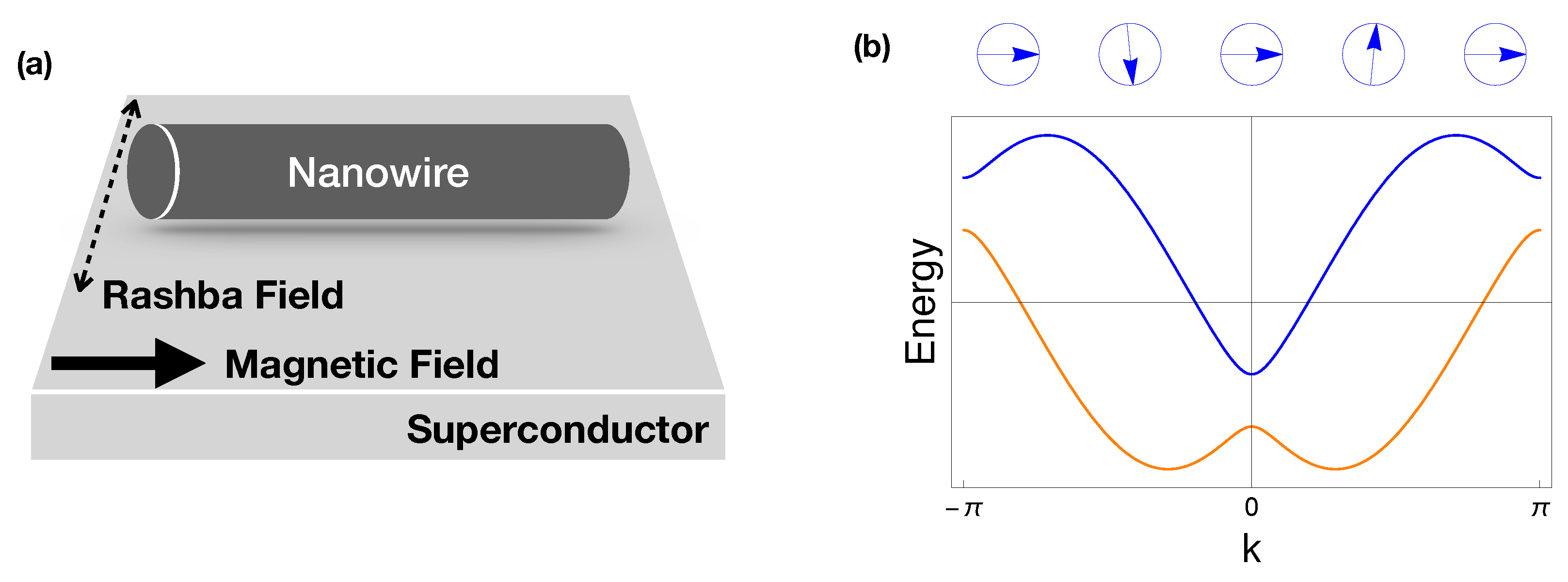
Figure 5.
(color online) Energy profiles of the two coupled Kitaev chains model as a function of inter-chain hopping, . The inter-chain pairing is set to zero, . (a) Ratio between the subgap state energy and bulk gap energy. The subgap energy is measured from the Fermi level. (b,c) Energy levels along the arrows in panel (a), i.e. complex phase of the hopping is fixed to , and in (b) and (c), respectively. The pure real corresponds to the nanowire model. Only the positive energy levels are shown. Parameters: The number of sites for a chains , on-site energy , (unit energy scale), intra-chain pairings , hoppings .
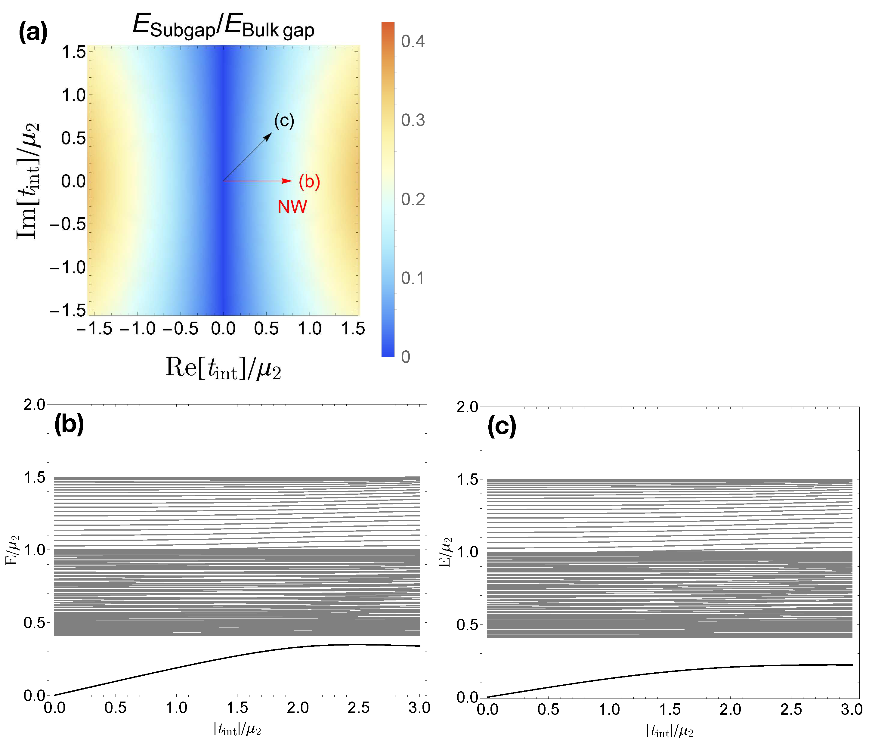
Figure 6.
(color online) Energy profiles of the two coupled Kitaev chains model as a function of inter-chain parametric pairing, , with inter-chain hopping at the boundaries. (a) Ratio between the subgap state energy and bulk gap energy. Inset arrows (Appx.1) is for the appendix. (b,c) Energy levels as function of with its complex phase are indicated as an arrow in panel (a). Parameters: The number of sites for a chains , on-site energy , (unit energy scale), intra-chain pairings , hoppings .
Disclaimer/Publisher’s Note: The statements, opinions and data contained in all publications are solely those of the individual author(s) and contributor(s) and not of MDPI and/or the editor(s). MDPI and/or the editor(s) disclaim responsibility for any injury to people or property resulting from any ideas, methods, instructions or products referred to in the content. |
© 2023 by the authors. Licensee MDPI, Basel, Switzerland. This article is an open access article distributed under the terms and conditions of the Creative Commons Attribution (CC BY) license (http://creativecommons.org/licenses/by/4.0/).
Copyright: This open access article is published under a Creative Commons CC BY 4.0 license, which permit the free download, distribution, and reuse, provided that the author and preprint are cited in any reuse.


