
You are currently viewing a beta version of our website. If you spot anything unusual, kindly let us know.
Preprint
Review
A Comparative Study on Recent Progress of Machine Learning-based Human Activity Recognition with Radar
Altmetrics
Downloads
104
Views
16
Comments
0
A peer-reviewed article of this preprint also exists.


This version is not peer-reviewed
Abstract
The importance of radar-based human activity recognition increased significantly over the last two decades in safety and smart surveillance applications due to its superiority towards vision-based sensing in the presence of poor environmental conditions, like illumination, increased radiative heat, occlusion, and fog. An increased public sensitivity for privacy protection, and the progress of cost-effective manufacturing, led to a higher acceptance and distribution. Deep learning approaches proved that the manual feature extraction that relies heavily upon process knowledge can be avoided by its hierarchical, non-descriptive nature. On the other hand, ML techniques based on manual feature extraction provide a robust, yet empirical based approach where the computational effort is comparatively low. This review outlines the basics of classical ML- and DL-based human activity recognition and its advances while taking recent progress of both categories into regard. For every category, state-of-the-art methods are introduced, briefly explained and discussed in terms of their pros, cons and gaps. A comparative study is performed to evaluate the performance and computational effort based on a benchmarking data set to provide a common basis for the assessment of the techniques’ degree of suitability.
Keywords:
Subject: Computer Science and Mathematics - Artificial Intelligence and Machine Learning
1. Introduction
In the last two decades, civil radar-based applications, as they are used for human sensing and human activity recognition (HAR), have made significant progress. This has been triggered and supported by the rapid development in semiconductor technologies in recent decades, in particular by the drastic change in the concept of radar. Modern radar systems are highly integrated, i.e. the most important circuits are housed on a single chip or a small circuit board.
The potential of radar-based sensing and recognition technologies has been discovered by a variety of different scientific domains and was the target of numerous preceding and recent research. First studies dealt with the detection of humans and recognition in indoor environments for application regarding security [1,2,3,4,5,6]. Medical applications, i.e. monitoring of patients extended its applicability [7,8,9,10,11,12,13] to sub-domains, e.g. vital sign detection. In addition, the latest developments of autonomous driving have impressively shown the enormous potential of radar-based automotive human activity and security applications, e.g. gesture recognition [14,15,16,17,18,19,20,21,22,23,24,25] and safety-oriented car assistance systems, e.g. fatigue recognition [26] or occupant detection [27,28,29,30,31,32], especially of forgotten rear-seated or wrongly placed infants or children, in order to prevent deaths due to overheating or overpowered airbags. In comparison to the aforementioned application field, automotive-specific applications suffer excessively by different environmental conditions due to the variation of light, temperature, humidity and occlusion. Further, increasing demands for privacy-compliant smart home solutions, e.g. for the intelligent control of heating [20] or the surveillance of elderly people in order to detect falls [9], have led to an unprecedented technological pace.
Although the advantages of vision-based sensing and recognition technologies are undisputed, there are many situations, where the drawbacks are severe, compared to radar-based technologies. Sensing-related problems comprise lighting conditions (poor illumination), thermal conditions (increased radiative heat), occlusion and atmospheric phenomena (fog, mirage). Besides those, radar-based systems are independent of privacy-related conditions, since target information do not rely explicitly on target shapes, but can be derived of microscale movements based on Micro-Doppler signatures [33,34,35,36,37,38].
The radar-based recognition of human activities has been studied by numerous authors, where classical Machine-Learning (ML) based techniques, e.g. k-Means [39], SVM [40,41,42,43,44] etc. as well as Deep Learning-based (DL) approaches have been used [45,46,47,48,49,50,51,52,53,54,55,56,57,58,59,60,61,62,63,64,65,66,67,68,69,70]. In general, ML-based techniques rely on shallow heuristically determined features that are characterized by simple statistical properties and thus, depend on technological experience. Furthermore, the learning process is restricted to static data and does not take long-term changes of the process data into consideration.
Deep Learning constitutes a subdomain of Machine Learning, where the methods applicability do not depend on the suitability of hand-crafted features. Feature extraction highly relies on domain knowledge and the the expertise of the user in particular. Instead, the deep learning approaches are able to extract high-level, yet not fully interpretable information in a generalized approach, and due to their structure, the underlying learning process can be designed to increase computational efficiency, e.g. by parallelization.
This work addresses the recent progress of ML-based HAR methods in radar technology setting and focuses on DL-based approaches, since those have proven to be a more generalized, long-term oriented, and robust solutions for classification problems. One major contribution of this paper is to provide the first comparative study of HAR methods using a common data base and a unified approach for the application of the most common DL methods while focussing on key aspects: CNN-, RNN- and CAE-based methods. The goal is to investigate the performance associated with computational cost, i.e. the total execution time and the space complexity, i.e. the parametricity of those methods under equal conditions in order to determine the suitability through comparison from which general recommendations can be derived. Furthermore, a unified approach for the classification task using different methods but a common preprocessing is proposed. The importance of careful preprocessing of the input data is provided by two variational studies. In the first study, the lower color value limit of the derived feature maps is varied and the impact on the accuracy is evaluated. This is important, since the characteristic patterns rely strongly on the color range, where high thresholds are associated with a higher degree of loss of important information, while low thresholds may contain redundant information, which, regardless of the model, could increase the risk of overfitting. In the second study, the impact of data compression of the feature maps on the accuracy is evaluated, since data reduction leads to lower storage requirements and hence reduced costs for hardware or faster data transmission rates for online systems.
The remaining sections are organized as follows: In Section 2, the basic principles of radar are outlined and briefly explained. Then, common preprocessing techniques are presented in Section 3, whereas Section 4 emphasizes on the recent progress of DL-based approaches after giving a short introduction. In Section 5, a comparative study of the most successful approaches and state-of-the-art methods of both preceding sections based on benchmark data are provided, where the performance, computational effort and the space complexity is evaluated and discussed in Section 6. Finally, the paper closes by presenting open research topics, derived by current gaps and challenging issues of the future.
2. Basic Principles
2.1. Radar-based Sensing
The underlying principle of the radar-based detection of targets, in general, is to emit and to receive electromagnetic waves (RF signals), which contain information about the targets properties. A common categorization of radar systems is to classify them into systems based on pulse radar or continuous wave. Both categories have their individual applications with specific advantages and disadvantages with regard to distance resolution, velocity resolution, power consumption, technical equipment, waveform generation, signal processing, etc.
2.2. Continuous Wave Radar
The main characteristic of Continuous Wave Radar systems (CW) is to emit a continuous electromagnetic wave using a sine-waveform, where the amplitude and frequency remains constant and to process the wave reflected by the target. Besides information about the reflectability, it contains information about the target’s velocity due to the Doppler frequency shift. A common variant of this technique are FMCW radar systems, whose waveform vary in the time-domain.
With regard to HAR, FMCW-based radar systems in the mm-wave domain have significant advantages compared to CW radar as the suitability for human sensing has been proven by numerous works in the last two decades [40,41,42,46,48,50,57]:
- High sensitivity: For the detection of human motions, especially for the small-scale motions, e.g. like breathing and gestures, a sensitivity close to the wavelength is required. This can be achieved when a high center frequency combined with a high bandwidth (B) is used.
- Minimized danger of multipath propagation and interactions with nearby radar systems due to the high attenuation of the mm-wave RF signal
- Distances and velocities of targets can be measured simultaneously, e.g. when triangular modulation of the chirp signal combined with a related signal processing technique is used.
- Independence to thermal noise as the phase is the main carrier containing information about targets distances
Figure 1.
Schematic representation of a FMCW-based radar sensor.
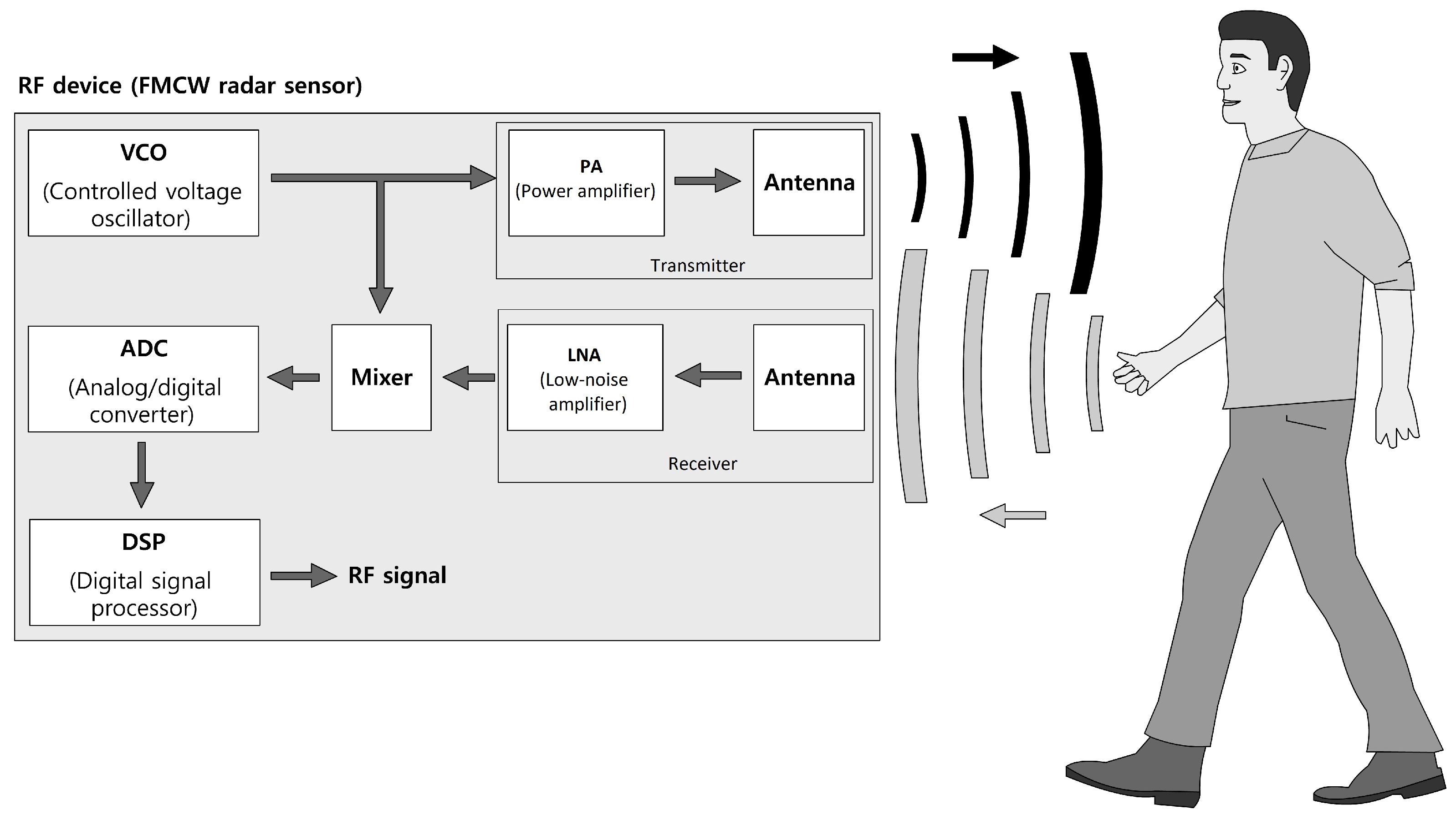
FMCW radar generate a sinusoidal power-amplified RF signal (chirp) by a high-frequency oscillating unit, where the frequency is varied linearly between two values and in sawtooth-like pattern over a certain duration according to the following function:
Figure 2.
Time-related characteristics of the chirp signal with sawtooth and triangular shape modulation.
Figure 2.
Time-related characteristics of the chirp signal with sawtooth and triangular shape modulation.
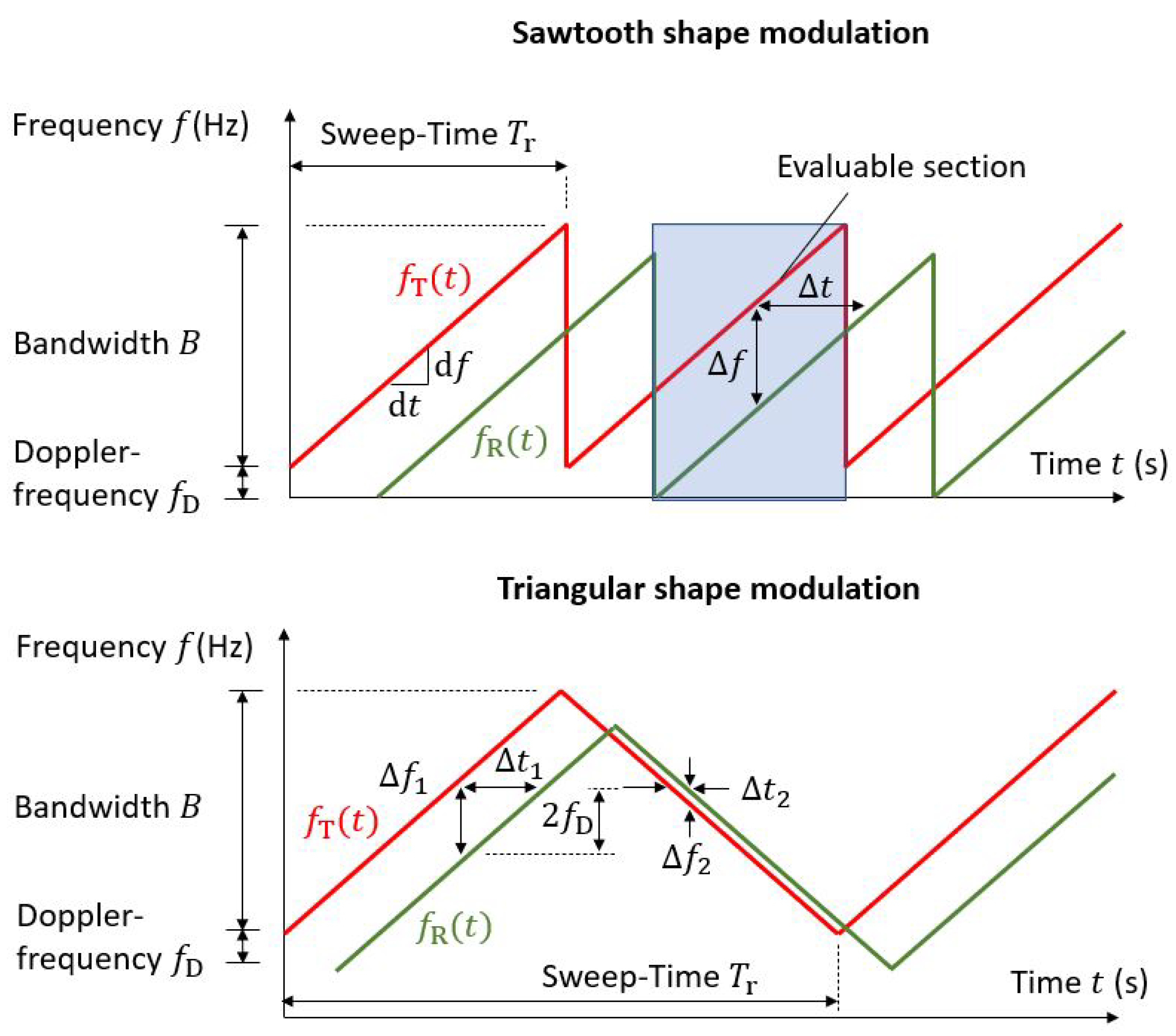
The constant / for determines the slope of generated signal, whereas the frequency variation is determined by a linear function. This RF signal is emitted via the transmitting antenna and the echo signal, which follows from the scattered reflection of the electromagnetic waves on the objects, are received at the receiving antenna and low noise-amplified. A mixer processes both, the transmitted and received signal, and generates a low-frequent beat signal, which, in the following, is preprocessed and used for the analysis.
A linear chirp signal that can be defined within the interval by
is emitted and mixed with its received echo signal to provide the IF signal
which, in the following, is preprocessed and used for the calculation of the feature maps.
In general, human large-scale kinematics, e.g. the bipedal gait, are characterized by complex interconnected movements, mainly of the body and the limbs. While the limbs have oscillating velocity patterns, the torso can be characterized by transitional movement solely.
According to the Doppler effect, moving rigid-body targets induce a frequency shift in the carrier signal of coherent radar systems that is determined in its simplest form by
where v is the relative velocity between the source and the target and the frequency of the transmitted signal. While the torso induces more or less constant Doppler frequency shifts, the limbs produce oscillating sidebands, which are referred to as micro-Doppler signatures [33]. In the joint time-frequency plane, these micro-Doppler signatures have distinguishable patterns, which make them suitable for ML-based classification applications. An example of can be found in Figure 3.
Micro-Doppler signatures are derived by time-dependent frequency-domain transformations. The first step is to transform the raw data of the beat signal to a time-dependent range distribution, referred to as the time-range distribution by the fast Fourier transform (FFT), where m is the range index and n the slow time index (time index along chirps).
While the Fourier-transformation is unable to calculate the time-dependent spectral distribution of the signal, the short-time Fourier transform (STFT) is a widely used method for the linear time-varying analysis that provides a joint time-frequency plane. In the time-discrete domain, it is defined by the sum of the signal values multiplied with a window-function, which is typically the Gaussian function to provide the Gabor transform:
Applied to the time-range distribution matrix , the time-discrete STFT can be computed by:
The spectrogram, also referred to as Time-Doppler Spectrogram (DT), is derived from the squared magnitude of the STFT:
Besides the STFT of the time-range distribution matrix, a FFT using a sliding window along the slow time dimension obtains time-specific transformation in the time-frequency domain, which are called range-Doppler distributions (RD).
A modification of the FMCW radar is the Chirp Sequence Radar [71]. It facilitates the unambiguous measurement of range R and relative velocity simultaneously, even in the presence of multiple targets. To do this, fast chirps of short duration are applied. The beat signals are processed in a twodimensional FFT to provide measurement of both variables by frequency measurements in the time domain t and the short-time domain k instead of a frequency and phase measurement, as it is the case for the regular FMCW radar. This method reduces the correlation between range and relative velocity and improves the overall accuracy.
2.3. Pulse radar
While the CW-based radar and its subclasses rely on moving targets to create micro-Doppler signatures, pulse radar is able to gather range information of non-moving targets, e.g. human postures by applying short electromagnetic pulses. A modification, which combines principles from both, CW and pulse radar, is pulse-Doppler radar.
In pulse radar, the RF signal is generated by turning on the emitter for a short period of time while switching to the receiver after turning of the emitter and listening for the reflection. The measuring principle is based on the determination of the round-trip time of the RF signal, which has to meet specific requirements with regard to the maximum range and range resolution that are determined by the pulse repetition frequency (PRF) or, alternatively, the interpulse period (IPP) and the pulse width (), respectively. A variant of pulse radar is Ultra-Wideband (UWB) radar, which is characterized by low-powered signals and very short pulse widths, which leads to a more precise range determination while having a drawback with regard to the Signal-to-Noise Ratio (SNR).
The reflected RF signals contain intercorrelated information about the target and its components, i.e. human limbs as well as the surrounding environments by scattering effects in conjunction with multipath propagation. Due its high resolution, small changes in human postures create different measurable changes in the shape of the reflected signal. Using sequences of preprocessed pulse signatures, specific activities can be distinguished between each other and used as features for the setup of classification models.
In [70], the authors developed and investigated a time-modulated UWB radar system to detect adult humans inside a building for security purposes. In contrast to static detection, [44] used the a bistatic UWB radar to collect data of eight coarse-grained activities for human activity classification. The data were collected at the center frequency of 4.7 GHz with a resolution bandwidth (RBW) of 3.2 GHz and a RBF of 9.6 MHz, which were reduced in dimensionality by the Principal Component Analysis (will be explained in the next chapter) and used within a classification task based on Support Vector Machine (SVM) after a manual feature extraction using the histogram of principal components for a short time window.
2.4. Preprocessing
In general, returned radio signals suffer from external incoherent influences, i.e. clutter and noise, and are therefore unsuitable for the training of machine-learning based classification methods. In addition to this aspect concerning the data quality, the success as well as the performance of classification methods depends on the data representation, the data dimensionality and the information density. Thus, it is necessary to apply signal processing techniques in order to enhance the data properties prior to the training and classification. The next subsection give a brief description of settled preprocessing methods.
2.4.1. Clutter
Radio signals reflected by the ground lead to a deterioration of data quality in general as it contains information unrelated to the object or the task. The difficulty for the determination and removal depends strongly on the situational conditions.
In static environments, the clutter can be removed by simply subtracting the data containing the relevant object from the data that were collected previously, where the object was missing [44]. Nevertheless, quasi-static or dynamic environments are characterized by changing conditions as they occur for mobile applications, storage areas etc. can affect the data.
Numerous works that emerged in the latest years, based their work on different approaches, e.g. sophisticated filters using eigenimages derived by Singular Value Decomposition (SVD) for filtering, combinations between Principal Component Analysis (which will be explained in Subsection E) as well as filtering in the wavenumber domain using predictive deconvolution, Radon transform or f-k filtering [74,75].
2.4.2. Denoising
One of the major problems for machine learning applications is called overfitting. It occurs when the model has a much higher complexity or degree of freedom with regard to the input data that was used for training. It leads to a perfect fitting to the training data but fails when other data, i.e. for testing, are considered.
To overcome this lack of generalization, when other factors can be excluded (e.g. the amount of data is sufficient), denoising is one the techniques to improve the accuracy. Using Low-pass filters, convolutional filters or model-based filters are the most common methods to reduce noise, which may mislead the algorithm to learn patterns that do not refer to the process itself.
Apart from that, adding noise may increase the robustness. In [61], Denoising Autoencoders (DAE) are used, where noise is added to the input data that leads to an overall increase of the models generalization ability. The most common method is to add isotropic Gaussian noise to the input data [62]. Another way is to apply masking noise or salt-and-pepper-noise, which means that a certain fraction of the input data is set to zero or changed to its corresponding maximum or minimum value, respectively [62].
2.4.3. Normalization
As the amplitudes of the target signatures depend substantially on the distance between sensor and the target, the normalization of the data is required in order to maintain consistent statistical properties, e.g uniform SNR, which are required for the training of ML models.
2.4.4. Data Reduction
The Principal Component Analysis (PCA) is a common method used for the reduction of the data dimensionality, which is beneficial for algorithms to learn efficiently [40]. Its main idea is to preserve the maximum variance of the data while projecting them onto a lower dimensional hyperplane using the first eigenvectors, called the principal components, where every predominant subset of principal components defines a plane, which is orthogonal to the following principal component (see Figure 4).
Due to its increased numerical stability, the Singular Value Decomposition (SVD) is a typical method for the calculation of the principal components :
To obtain a reduced dataset, the first m principal components, where the cumulated explained variance ratio exceeds a certain target threshold, are selected to form a matrix, which is multiplied by the original data matrix:
2.4.5. Whitening
Closely related to the normalization, whitening refers to a more generalized method, where a transformation is applied to input data so that the diagonal elements of the covariance matrix are all ones (also called sphering). This method reduces the correlation between the input data and improves the efficiency of the learning algorithm. The most common methods in connection with that are the Principal component analysis (PCA), the Zero-Phase Component Analysis Whitening (ZCA) and the Cholesky Decomposition [72,73].
The Prinicipal Component Analysis is the most popular procedure for decorrelating data, which can be used to reduce the dimensionality of data while the variance of data is maximized. With regard to twodimensional data structures, like e.g. images, this is achieved by determining the covariance matrix, which is decomposed using the SVD into two orthogonal matrices and one diagonal matrix , where the diagonal matrix contains the eigenvalues. Taking only the first n components of the eigenvector matrix along with their corresponding eigenvalues it is possible to obtain a compressed version of the original image. Here, it is used to compute the conversion matrix , which can be multiplied with the original matrix to achieve decorrelation:
The small constant , which is usually around is inserted to avoid large coefficients that are caused by the reciprocal of very small eigenvalues. The zero-phase transformation
is a whitening procedure, where the transformation leads to uncorrelated data with, in contrast to the PCA, unit variances and is computed using the PCA and an additional multiplication with the eigenvector matrix .
2.5. Feature Engineering
In general, the selection and extraction of features during feature engineering is crucial for the success of machine learning applications. The term selection refers to the identification of strongly influencing measurable properties with regard to the mathematical task while extraction deals with the dimensionality reduction when using compositions of features. For example, in [40], the PCA is used to determine the histogram of the most influencing PC for given time window, from which the mean and variance are used as features. Another example is [37], where the number of discrete frequency components are determined using spectrograms that contain micro-Doppler signatures, which provides useful information about the location of small-scale motions.
Classical techniques, e.g. Linear Regression, Decision Trees, Random Forests, k-Nearest Neighbor, etc. rely heavily on handcrafted feature engineering, which implies a certain experience and domain-knowledge, while DL methods use algorithms that select useful features automatically, which, as a main drawback are hardly interpretable by humans and indirectly evaluable.
2.6. Challenges
Besides the numerous convincing applications of machine-learning methods to human activity recognition, there are still topics that haven’t been investigated yet or at least, have only been partially addressed. In general, these challenges can be divided into source-related problems and methodological problems that are presented in the following subsections.
The first source-related problem deals with the fact that related works pursue different aspects of human activity recognition and rely on own data acquisition, which is depending on the activities the authors focus. Different data sets with varying activities of different scale constitute a major problem, as the condition for comparability is simply not given, e.g. [40,41,42,48,50,53,57,59] use coarse-grained activities for their investigation while [26,46] use fine-grained activities as a basis for their works. Especially, the last point states a problem, since the movements are linked to weaker micro-Doppler signatures in terms of power.
Another problem is that many activities of both degrees of fineness classes have a certain similarity, which has been proven, e.g. by [40], where data collected from coarse-grained activities were used for a SVM-base binary classification problem and activities like punching were confused with running.
Among other factors, every activity has its unique micro-Doppler signature, so machine learning-based classification models are trained to distinguish between the specific activities, but not for the transitions between them, which leads to performance losses especially for online applications.
Human activities can be broadly classified into two main categories: Coarse-grained and fine-grained activities. For constant configurations regarding data acquisition, this leads to different magnitudes and distributions of local variations, which lead to a different classification accuracy.
As humans have individual physical properties due to genetics, age, sex, fitness, disabilities, consequences of illnesses or surgeries, etc., which change over time, the datasets will also have variances in the amplitude or time-domain, which leads to individual, temporal micro-Doppler signatures.
In general, micro-Doppler signatures contain information of the person activity characteristics. Besides the difficulties mentioned above, the complexity of the classification task is severely affected by the number of subjects, when the classification is not broken down to subordinate, composite classification tasks based on datasets for every single individual. This problem is exacerbated by different activities being performed simultaneously.
Many human activities consist of sequential, subdivided activities, e.g. lifting a blanket, rotating from the horizontal into a sitting position and standing up is connoted with the wake up process. As the whole sequence is required to form the dataset for that specific activity, the segmentation plays an important role for the data preprocessing.
As single activities lead to similar data sets for each repetition, the complexity of the classification task is increased when the data sets are collected from concurrent activities. Signatures containing smeared patterns lead to data sets with ambiguous characteristics of high variance.
Models for classification problems rely on large amounts of data for the training and validation, which require a consistent annotation. While for experimental conditions this is not the case, data collection from public sources for an adaptive online application have to be labelled.
Due to clutter, the data quality is strongly degraded by the presence of nearby objects, which reflect fractions of the emitted power to the receiver by multipath propagation. For mitigation, data from the environment are collected and used for the preprocessing. For mobile applications, this is a crucial topic as the surroundings do not remain constant.
The handcrafted selection of significant unique features is one of the major problems of classical machine learning classification problems, as this requires time consuming efforts to find distinguishable patterns in the data, so that the risk for the confusion of similar activities is significantly reduced.
Data used for the training are collected by repeating executions of planned activities by multiple subjects, e.g. running, jumping, sitting etc. Unplanned, uncomfortable actions, e.g. falling, are much rarer events, which leads to unequal class batch sizes.
3. Review of Methods
3.1. Support Vector Machine
The numerically optimized and generalized method was developed by Boser, Guyon and Vapnik in the nineties [49] while the basic algorithm behind Support Vector Machines (SVM) was introduced by Vapnik and Chervonenkis in the early sixties [51]. With regard to its application to classification tasks, the main idea is to introduce hyperplanes using a so-called kernel-trick, which maps points in a nonlinear way into a higher-dimensional space, so that the margin between those and the hyperplanes is maximized increasing their separability. Its suitability to human activity recognition classification tasks and great potential was confirmed by numerous authors.
In [40], a bistatic UWB radar system working at 4.3 GHz has been used to obtain datasets of time-based signatures of human interaction with the radar signal to train SVM based on the one vs. one method for the classification of seven activities that have been performed by eight subjects: walking, running, rotating, punching, crawling, standing still and a transition between standing and sitting. The data was significantly reduced by 98.7 % using the PCA, where the main 30 coefficients have been selected. The classification accuracy reached only 89.88 % due to difficulties resulting from the confusion as certain activities have similar micro-Doppler signatures.
In a recent study, Pesin, Lousir and Haskou [42] studied radar-based human activity recognition using a sub-6GHz and a mmWave FMCW radar system. Based on SVD, three-dimensional features, consisting of the minimum, maximum and the mean function of the matrix , were derived from range-time-power signatures and used for the training of a Medium Gaussian SVM, which was applied to classify three different activities (walking, sitting, falling). With an average classification accuracy of 89.8 % for the mmWave radar system as well as 95.7 %, it was shown that radar systems with a higher resolution do not necessarily lead to a better classification.
3.2. Convolutional Neural Networks
Since their introduction in the 1980s by Yann LeCun, Convolutional Neural Networks (CNN) gained importance in science, especially in the signal processing domain. As for other scientific fields, e.g. computer vision or speech recognition, the application of CNN has been carried for human activity recognition by numerous works in the last decades [40,41,48].
Convolutional Neural Networks are architectures that consist of stacked neural layers of certain functional types. The basis is formed by sequences of Convolutional layers and pooling layers. Convolutional layers are sets of convolutional filters, which connect neurons of the current layer with local sections (receptive fields) of the previous layer or input layer (see Figure 5). The filters apply a convolution based on the size of the receptive fields, the stride and the weights to the neurons of the previous layers, which is called feature extraction, in order to create feature maps using activation functions, e.g. ReLU, sigmoid, tanh etc. Feature maps contain information about the most active neurons with regard to the specific filter. The two-dimensional discrete convolutional is applied using the following general formula
where K is the kernel along with the indices and I is the input or preceding layer with the indices , accordingly.
The determination of the weights of a filter is the main task of the learning process and in contrast to fully-connected networks (FCN), this structure reduces the amount of weights and therefore the computational effort significantly and preserves a certain degree of generalization. Pooling layers perform a subsampling task in order to reduce the amount of information and therefore the computational load and to increase the degree of invariance towards slight variations of the data of previous layer. The most common pooling layer types are the maximum pooling layer and average pooling layer, where the first one selects the neuron of the highest value within its specific receptive field and the latter takes the average value of all neurons of the receptive field of the previous layer. At the end, fully connected layers connect the neurons that contain the results of the convolutional process to the neurons of the output layer of a classification task by flattening. The degree of generalization can be increased by inserting dropout layers, which reduce the number of neurons.
Seyfioglu, Özbayoglu and Gürbüz [53] applied multiclass SVM, AE, CNN and CAE to classify 12 aided and unaided, coarse-grained human activites. Using a 4.0 GHz CW radar system to create spectograms, domain-specific features, e.g. cadence velocity diagrams (cvd) among non-domain features, e.g. cepstral coefficients, LPC and DCT were derived. The sample sizes ranges from 50 (sitting) to 149 (wheelchair) for each class. The CAE-based approach achieved the highest accuracy of 94.2 %, followed by the CNN (90.1 %), the AE (84.1 %) and multiclass SVM (76.9 %).
Singh et al. [48] used time-distributed CNN enhanced by bidirectional LSTM to classify five human full-body activities, consisting of boxing, jumping, jacks, jumping, squats and walking, based on mm-wave radar point clouds. The data set was collected via a commercial-of-the-shelf FMCW radar system in the 76–81 GHz frequency range that is capable of estimating the target direction. The data set consists of 12,097 samples for training, 3,538 for testing and 2,419 for validation, where each sample consists in a voxelized representation with a dimensionality of . Among the other ML-based methods applied (SVM, MLP, Bidirectional LSTM), the achieved accuracy of 90.47 % is the highest. However, the main drawback of this method is the increased memory requirement for the voxelized representation of target information, which is not a concern when using micro-Doppler signatures.
Besides Stacked Autoencoders and Recurrent Neural Networks, Jia et al [41] applied CNN to a data set that has been collected by a FMCW radar system working at 5.8 GHz. The dataset was used to build features based on compressed data of the dimensionality for range-time, Doppler-time amplitude and phase, and cadence velocity diagram [41]. The data were collected from 83 participants performing six activities, consisting of walking, sitting down, standing up, picking up an object, drinking and falling, which were repeated thrice to deliver 1,164 samples in total. An accuracy of 92.21 % was achieved for the CNN using Bayes optimization, while the SAE yielded 91.23 %. The SVM-based approach yielded 95.24 % after a feature adaptation using SBS while the accuracy of the CNN was improved to 96.65 % by selecting handcrafted features.
Huang et al. [63] used a combination between a CNN and a Recurrent Neural Network (LSTM) model as a feature extractor from point-cloud-based data and a CNN to extract features from range-Doppler maps. Outputs from both models were merged and fed into a FCN-based classifier to classify the inputs into 6 activities, consisting of in place actions, e.g. boxing, jumping, squatting, walking, and high-knee-lifting. The results show a high a very high accuracy of 97.26 %, which is higher than using the feature extraction methods in separate approaches.
In [64], a CNN-model was developed using two parallel CNN-networks whose outputs are fused into a FCN for classification (DVCNN). This approach along with an enhanced voxelization method led to high accuracies, which are 98 % for fall detection and 97.71 % for activity classification.
Chakraborty et al. [65] used open-source pre-trained DCNN, i.e. MobileNetV2, VGG19, ResNet-50, InceptionV3, DenseNet-201 and VGG16 to train with an own provided dataset (DIAT- RadHAR) that consists of 3,780 micro-Doppler images comprising different coarse-grained military-related activities, e.g. boxing, crawling, jogging, jumping with gun, marching, and grenade throwing. An overall accuracy of 98 % proved the suitability of transfer learning for HAR.
3.3. Recurrent Neural Networks
Since the works of Rumelhart, Hinton as well as Williams [77] and Schmidhuber [76], Recurrent Neural Networks (RNN) and derivates, i.e. Long-Short Term Memory Networks have been widely applied in the fields of natural sciences and economics. In contrast to CNN, which are characterized as neural networks working in a feedforward manner since their outputs are depending strictly on the inputs, RNN have the ability to memorize their latest states, which make them suitable for the prediction of temporal or ordinal sequences of arbitrary lengths. They consist of interconnected layers of neurons, which use the current inputs and the outputs of the previous time steps to compute the current outputs with shared weights allocated to the inputs and outputs separately using biases and nonlinear functions. By stacking multiple RNN layers, a hierarchy is implemented, which allows the prediction of more complex time-series.
An exemplary structure of a RNN is presented in Figure 6. In the left part, the network architecture is presented in a general notation, while in the right part its temporal unrolled (or unfolded) presentation is illustrated, where each column represents the same model, but for a different point in time. The current input is required to update the first hidden state of the node i, where i and t denotes the node index and the time instance, respectively, along with the previous state of the same node using the weighting matrices and a nonlinear activation function for the output. Then, the output of the node is passed to the next hidden state as an input using the weighting matrix . Last but not least, the models output is obtained using another nonlinear activation function. This leads to a structure of interlinked nodes that are able to memorize temporal patterns, where the number of nodes determines the memorability.
Besides their enormous potential for the prediction of complex time series, RNN suffer from two main phenomena, called unstable gradients and vanishing gradients, which limits their capabilities. The first phenomenon occurs when a complex task affords many layers, which lead due to the accumulation of increasingly growing products to exploding gradients while the second refers to the problem that the cells, due to their limited structure, tend to reduce the weights of the earliest inputs and states.
3.4. Long-Short Term Memory (LSTM)
In 1997, Hochreiter and Schmidhuber [78] introduced LSTM cells, which have been investigated and enhanced by additional works of Graves, Sak, Zaremba [80,81,82]. In contrast to the RNN, Long Short-Term Memory networks are efficient in managing longer sequences and able to reduce the problems that lead to the restricted use of simple RNN. A LSTM cell contains short-term and long-term capabilities, which enables the memorization and recognition of the most significant inputs using three gate controllers (see Figure 7).
The input gate controls which fraction of the main layer output using the input is used for the memory. For Peephole Convolutional LSTM, which is a variation of the standard Peephole LSTM to be suitable for processing images, it is calculated using the current input , the previous short-time memory and the past long-time memory that are multiplied with the corresponding weighting matrices , , and using matrix multiplication or element-wise multiplication (denoted as * and ∘, respectively) and passed to a nonlinear function along with a bias term (see Eq. 17). In contrast to the input gate, the forget gate defines the fraction of the long-term memory that has to be deleted. Similarly, the input and both memory inputs are multiplied with the matrices , , and , respectively, and added to another bias term, prior to being passed to the same nonlinear activation function (see Eq. 16). This forms the basis for the updates of the memory states, where the current long-time memory (or cell state) is calculated as the sum of the previous long-time memory being weighted by the forget gate and the new candiate for the cell state, which is the tanh-activated linear combination of the weighted input and the previous short-time memory being weighted by the input gate (see Eq. 18). Finally, the output gate determines the part of the long-term memory that is used for the current output and as the short-term memory for the next time step. For this, the current short-time memory of the LSTM-cell is calculated by the tanh-activated current long-time memory weighted by the output gate, which itself is calculated using the current input, the past short-time state and the current long-time memory state (see Eqs. 19 and 20).
Vandermissen et al. [46] used a 77 GHz FMCW radar to collect data of nine subjects performing 12 different coarse- and fine-grained activities, namely, events and gestures. Using sequential range-Doppler and micro-Doppler maps, five different neural network types, consisting of LSTM, 1d-CNN-LSTM, 2d-CNN, 2d-CNN-LSTM and 3d-CNN, have been investigated using the 1,505 and 2,347 samples for events and gestures, respectively, with regard to performance, modality, optimal sample length and complexity. It was shown that the 3d-CNN resulted in an accuracy of 87.78 % for the events and 97.03 % for the gestures.
Cheng et al. [57] derived a method for through-the-wall classification and focussed on the problem of unknown temporal allocation of activities during recognition, which has a significant impact on the accuracy. By employing Stacked LSTMs (SLSTM) embedded between two fully connected networks (FCN) and using randomly cropped training data within the Back Propagation Through Random Time (BPTRT) method for the training process, an average accuracy of 97.6 % was achieved for the recognition of four different coarse-grained activities (punching three times, squat and pick up an object, stepping in place, raise hands into horizontal position).
In [59], a SFCW radar system was employed to produce spectrograms for multiple frequencies collecting data of 11 subjects that were performing six different activities with transitions. By comparing single-frequency LSTM and Bi-LSTM with their multi-frequency counterparts, it was shown that the classification performance was significantly higher, resulting in 85.41 % and 96.15 % for the accuracy.
Due to their ability to memorize even longer temporal sequences, what applies for a wide range of human activities, LSTM networks are in general suitable for radar-based HAR as long as the limitations are considered. The limits that RNN also have to deal with, i.e. the numerical problems with the determination of gradients, set up constrains to the sample lengths of input data [46]. Moreover, in comparison to other techniques, LSTM require a high memory bandwidth, which can be a major drawback for online applications if hardware with limited resources is used [79].
3.5. Stacked Autoencoder
For a variety of applications, dense or compressed representations of input data using unlabeled data are required to reduce the dimensionality based on an automatic extraction of significant features. Autoencoders and modifications of those have proven their suitability for a variety of fields, especially in the image processing domain. A basic Autoencoder (AE) consists of an encoder, which determines a latent representation of the input data in one hidden layer of much lower dimensionality (codings), and the decoder, which reconstructs the inputs based on these codings. Using Stacked Autoencoders (SAE) that have multiple symmetrically-distributed hidden layers (stacking) the capability to cover inputs, which require complex codings, can be extended (see Figure 8).
Jokanovic et al. [8] used SAE for the feature extraction and a softmax regression classifier for fall detection. Besides the positive effect of the proposed preprocessing method, the results show a good accuracy of 87 % accuracy.
Jia et al. [41] used SAE, besides SVM and CNN, to evaluate the performance using multidomain features, i.e. range-time (RT), Doppler-time (DT) and Cadence Velocity Diagram (CVD) maps based on the open dataset [35] and an additional dataset. It could be shown that for different feature fusions CNN was the most robust method, followed by the SAE and lastly SVM.
3.6. Convolutional Autoencoder
When useful features of images found the basis for an application, Convolutional Autoencoders (CAE) are better suited than SAE due to their capability of retaining spatial information. The high-level structure equals that of a simple Autoencoder, namely the sequence of an encoder and a decoder, but in this case, both parts contain CNN (see Figure 9).
Campbell and Ahmad [56] pursued an augmented approach, where a Aonvolutional Autoencoder was used for a classification task using local-feature maps for the convolutional part while the whole signature is for a multi-headed attention part (MHA). The MHA is an aggregation of single-attention heads, each head being a function of the three parameters query, key and value. The dataset was established by using a 6 GHz Doppler radar to collect data from five subjects based on the coarse-grained activities fall, bend, sit and walk [56], where each activity was repeated six times. The study was carried out for different training and test split sizes. From the results, it was derived that the attention-based CAE required less data for training than the standard CAE of up to three layers and achieved an accuracy of 91.1 % for the multi-headed attention using a multi-filter approach.
A comprehensive overview over key articles with regard to their radar technology domain, data, classification method, and achieved results is provided in the Table A1, which can be found in the Appendix A.
3.7. Transformers
In 2017, Vaswani et al. introduced a new deep learning model, called transformer, whose purpose was to enhance encoder-decoder models [66]. Originally derived for sequence-to-sequence transductions, e.g. in Natural Language Processing (NLP), transformers gained importance in other fields, too, e.g. image processing due to their ability to process patterns as sequences in parallel, to capture long-term relationships and, therefore, to overcome the difficulties that CNN and RNN-based models have. They consist of multiple encoder-decoder sets, where the encoder is a series of a self-attention layer and a feed forward neural network, while the decoder has an additional layer, the encoder-decoder attention layer, which helps to highlight different positions while generating the output.
Self-attention mechanisms are the basis of transformers. In the first step, they compute internal vectors (Query, Key, and Value) based on the products of input vectors and weighting matrices, which are then used for the calculation of scores after computing the dot products between the query vectors and the key vector of all other input vectors. The scores can be interpreted as the focus intensity. Using the softmax function after a normalization, the attention is calculated as the weighted sum of all value vectors. The weighting matrices are the entities that are tuned during to training. Using multiple (Multihead) self-attention mechanisms (MHSA) in parallel, it is possible to build deep neural networks with complex dependencies.
Transformer have been applied in radar-based human activity as well. In [67], a transformer was trained as an end-to-end-model and used for the classification of seven coarse-scaled tasks, i.e. standing, jumping, sitting, falling, running, walking, and bending. In comparison with the two other benchmark networks, the accuracy was the highest with 90.45 %. Focussing on making transformers more lightweight, in [68], another novel transformer was developed and evaluated based on two different datasets of participants performing five activities, e.g. boxing, waving, standing, walking, and squatting with an accuracy of 99.6 % and 97.5 %, respectively. Huan et al. introduced another lightweight transformer [69], which used a feature pyramid structure based on convolution, which was combined with self-attention mechanisms. The average accuracy for the public and own dataset was 91.7 % and 99.5 %, respectively.
4. Comparative Study
As the investigation of performance of recently investigated DL-based approaches is obtained by individual studies, which rely mainly on differing data sets, this paper attempts to enforce comparability by establishing a common basis using the same dataset for a variety of DL methods. In the first study, all models are trained and evaluated using the same dataset and good practical knowledge. An additional study is conducted to highlight the importance of a careful preprocessing, i.e. the adjustment of color value limits of the feature maps using threshold filtering, where the lower limit is varied using three different offsets, i.e. -30, -50, and -70 with regard to the maximum color value, and the influence on the classification accuracy is investigated. A second study is conducted where the influence of compression on the feature maps on the accuracy of the selected models is investigated for three compression ratios.
4.1. Methodology
The methodology is expressed through a flowchart that describes the basic procedure (see Figure 10). In the first step of the preprocessing, the dataset is used to generate the images containing the feature maps, i.e. time-Doppler maps. After scaling and trimming, the color levels are adapted. In order to reduce dimensionality, the colors are converted to grayscale. Using compression, the image size is reduced. Whitening is performed to decorrelate the data without reducing the dimensionality. Hereafter, the dataset is split into training, validation and test data sets. In the model setup, the model for the classifier is defined and, depending on the model architecture, an additional model for the pretraining is defined, if necessary. The procedure closes with the evaluation of the model. Since the classes are balanced, the performance metrics accuracy, recall and the confusion matrix are suitable for evaluation.
4.2. Dataset
In this study, the open dataset Radar signatures of human activities [35] will be used, which was lately the basis by Zhang et al. [83] to produce hybrid maps and to train the CNN architectures LeNet-5 and GoogLeNet for classification and benchmarking using transfer learning, respectively. Jiang et al. [54] used this dataset for a RNN-based classification using a LSTM-based classifier, which achieved an average testing accuracy of 93.9 %. Jia et al. [41] used this dataset for the evaluation of SVM-based classification with varying kernel functions achieving accuracies between 88 % and 91.6 %.
The dataset consists of a total of 1,754 data samples, stored as .dat files, which contain raw complex-valued radar sensor data of 72 subjects in the age of 21 to 88 who are performing up to six different activities, i.e. drinking water (index 0), falling (index 1), picking up object (index 2), sitting down (index 3), standing up (index 4), and walking (index 5) [35] (See Table 1). The data were collected using a 5.8 GHz Ancortek FMCW radar, which has a chirp duration of 1 ms, a bandwidth of 400 MHz, and a sample time of 1 ms. Each file, which is either about 7.5, 15 or 30 MB in size, contains the sampled intermediate radar data of one particular person performing one activity at a specific repetition.
It must be noted that there is a class imbalance. The activity class falling (index 1) consists of a total of 196 sample images, while the others have 309 or 310 sample images.
4.3. Development Platform
The study was conducted using an Intel Core i7-1165G7 processor that is accompanied by an Intel Iris Xe graphics card. The embedded graphics card is capable of using 96 execution units at 1,300 MHz. 16 GB of total workspace is available.
The methods were developed using Python-based open source development plattforms and APIs, i.e. TensorFlow, Keras, and scikit-learn, among basic toolboxes, e.g. numpy, pandas and others.
4.4. Data Preprocessing
The data was converted to Doppler-time maps in the JPEG-format using a Python script that was developed considering the hosted MATLAB file. The function transforms the sampled values of the raw radar signal into a spectrogram. In the first step, the data is used to calculate the range profile over time using a FFT. Then, a fourth-order Butterworth filter is applied and the spectrogram is calculated using a second Fourier-tranformation being applied on overlapping time-specific filtering windows, i.e. Hann window. Subsequently, the spectrograms are imported in the Python-based application and transformed to images of px in size after scaling. Trimming the edges and adapting the color levels is important to remove weak interfering artifacts and to highlight characteristical patterns, caused by frequency leakage or non-optimized windowing. In the next step, they are converted to grayscale images to reduce dimensionality, since the color channels do not contain any additional information in this case. A compression using a truncated SVD is applied to reduce data size while the main information is kept.
Using the ZCA method, the images are whitened. Dimensionality reduction is discarded to avoid significant loss of information. As the colors values range from 0 to 255, a normalization is applied afterwards that scales the values from 0 to 1 in order to improve the performance.
4.5. Model Setup
For the assessment, a variety of models out of three deep learning classes were implemented: Convolutional Neural Networks (CNN), Recurrent Neural Networks (RNN) and Convolutional Autoencoders (CAE) with fully-connected networks.
The CNN model consists of three instances of 2D Aonvolutional layer, where each of them is followed by maximum pooling layer and a dropout layer. Hereafter, the network closes with a flattening layer for implementing vectorization and connecting to two fully-connected layers (see Figure 12). It was implemented based on the Keras Sequential API using the layer functions Input, Conv2D, MaxPooling, Dropout, Flatten, and Dense, the optimizers SGD and Adam as well as the loss function Categorical Crossentropy from the packages keras.layers, keras.optimizers, and keras.losses, respectively.
The increasing number of filters of each Convolutional layer helps to build up hierarchical features and to prevent overfitting since the first layers capture low-level information while the last ones reach a higher level of abstraction but higher complexity and becoming smaller to enforce generalization. The 3-by-3-kernel of stride 1 without padding is required to halve the dimensions of the feature maps until the smallest size is reached that produces good results, which is 28 x 28. The values for the penalty function of the regularizers for the kernel, bias, and activity are set to be , , and , which are good empirical values to start with. The activation function was selected to be Rectified Linear Units (ReLU) for faster learning. The comparably average dropout rate of 0.4 is well-suited for this network, since the aforementioned regularizers must be taken into account. The first downstream FCN, which consists of 212 nodes and is connecting the last maximum pooling layer with the output FCN, is used for the classifier. It is required to transform the spatial features of the feature maps into complex relationships. The output FCN has six nodes, each one representing one class and using a Softmax activation function for determining the probability of class assignment for the input image.
RNN models were realized by networks of simple RNN, LSTM, Bidirectional LSTM as well as Gated Recurrent Units (GRU), which are implemented based on the Keras Sequential model, too, using the layer functions SimpleRNN, LSTM, GRU, Bidirectional, and Dense from the package keras.layers.
The number of nodes of the first part, which is the recurrent network, was uniformely set to 128, which leads to good results and prevents overfitting. For activation, the hyperbolic tangent function (tanh) was selected, which is associated with bigger gradients and, in comparison with sigmoid function, faster training. Each network is followed by a fully-connected layer to establish the complex nonlinear relationships that is required to connect the time-specific memory with the classes. Using a softmax function for activation, the probabilities are outputted for each class.
The autoencoder-based model architecture is implemented based on the CAE (see Figure 13). In contrast to the aforementioned implementation, it uses the Keras functional API, which is more flexible, as it allows branching and varying numbers of inputs and outputs. The branching option is required to define the encoder and decoder part independently from each other, since it requires two consecutive training sessions. The first training (pretraining) is performed on the complete autoencoder model that consists of the encoder part and the decoder part, to train the feature-extracting capabilities. After that, the trained weightings and biases are transferred to a separate model that consists of the encoder part and a FCN, which implements the classifier, to output the class probabilities.
4.6. Training
Using a percentage of 70 % for the size of the training subset on the total training dataset, the training was carried out based on cross-validation using batches of 32 samples for up to 300 epochs. For the validation, a percentage of 20 % was defined, hence 10 % of the data set remain for the test subset. The model-specific numbers of parameters are listed in Table 2.
Depending on the network, the optimizer was either based on the Stochastic Gradient Descent algorithm (SGD) or Adam (adaptive moment estimation) using individual and optimized learning rates for every network, varying between and .
5. Results
For the evaluation of the performance, the standard ML scores accuracy, recall, precision, F1-score were selected. Due to the class imbalance, i.e. unequal sample size between the activity falling (index 1) and the others, the measures accuracy, recall, and precision will tend to have slight errors, which is of subordinate relevance, since the relations are of main interest. The F1-score has the robustness to overcome this issue, since it compensates the tendency of the recall to underestimate and the precision to overestimate using the harmonic mean calculated from both. The two additionally provided scores macro-averaged Matthew Correlation Coefficient (MCC) and Cohen Kappa are robust against class imbalance, too, and, along with the F1-score, they form the basis for the assessment. The MCC, which has its origin in the binary classification, can be used to evaluate the classifier performance in a multiclass classification task, when a one-vs-all strategy is pursued. In this case, the classifier performance is computed using the average of the performance of every classifier, where each one can only classify a sample as belonging to the class assigned or, conversely, as belonging to any of the remaining classes. The Cohen Kappa measures the degree of agreement of different classifiers, where in this case, the probabilities of agreement between the classifiers in a one-vs-all strategy along with the probabilities for a random-driven agreement are considered.
The metrics of the results of the classification studies are listed in Table 3. The learning curves, consisting of the loss and accuracy function, as well as the resulting confusion matrices are displayed in the Figure 14, Figure 15, Figure 16, Figure 17 and Figure 18.
The learning curves of CNN (Figure 14) show a moderate learning pace with decreasing variance and likeliness of sudden spikes that are likely to appear when using the Adam optimizer. The decreasing gap between the training and validation curves indicate the absence of overfitting. From the confusion matrix, it is observable that there is a higher probability for the network to confuse the activity picking up objects with drinking, while the other tasks remain unaffected.
The RNN-based networks show varying performances. The LSTM network has similar learn curves with regard to learning pace and generalization and the confusion matrix shows the same issue like the CNN. The learning curves of the Bi-LSTM have a significant faster convergence but suffer from higher variances, as the confusion is significantly smaller with regard to the aforementioned models. The GRU network shows a higher tendency towards overfitting with comparably small variances in the accuracy progress. Last but not least, the CAE network shows the biggest tendency to overfitting and, besides to the confusion between tasks 0 and 2, there is an increased risk for confusing tasks 0 (drinking) with 4 (standing up).
The influence of the color levels of the feature maps on the performance is shown in Figure 19. The variational study was carried out for all models, where the lower limit of the color limits was varied using the offsets -30 (least details), -50, and -70 (most details) with regard to the maximum color value. Here, CAE and CNN show the best performance and higher robustness towards color level variations while the RNN-based methods are strongly affected with the GRU showing the strongest effects. The results indicate that the color levels have a great impact on the classification accuracy. Considering the stochastic effects of the training, in this study, the optimum lies probably between -50 and -70.
The influence of compression ratio of the feature maps on the performance is shown in Figure 19. Using three different compression ratios, i.e. 100 %, 67 %, and 50 %, the study was carried out for all models. According to the results, the performance of all models except the GRU shows a high robustness towards information loss caused by compression with the CAE achieving the best results, followed by the CNN and the Bi-LSTM. In practice, this means that even with a halfed data size the models are able to reach a similar performance. It must be taken into account that the model-specific performance deviations for the investigated cases are caused by the stochastic property of the learning algorithm and the dataset batching process.
From the results, we can confirm that the CNN-based classification has better performance in comparison to the investigated RNN-based methods. The reason for this is that the derived feature maps of the CNN have the ability to extract locally-distributed spatial features in a hierarchical manner and, therefore, to recognize typical patterns, whereas the RNN-based methods memorize temporal sequences of single features. This ability applies for the CAE, too, but the tendency for overfitting is much higher, so that tuning, e.g. through better regularization, is necessary. For the underlying type of input, namely images, the RNN-based networks are suboptimal due to the lack of scalability and the absence of memorizing spatial properties.
Further, it could be revealed that the classification of coarse-grained activities leads to better results. Higher magnitudes of the reflected radar signal, which are assigned to large-scale movements, lead to distinct characteristic properties in the micro-Doppler maps, which improve the performance.
6. Discussion
According to the metrics of the validation, all models provided acceptable results for the same dataset that indicated their overall suitability for this application with different performances. In addition, the learning curves of all models were convergent, but indicated different levels of smoothness and generalization. Further, it could be confirmed that the misclassification for all models was the highest between the activities drinking (index 0) and picking up objects (index 2).
The results show that CNN are more suitable structures for the given task compared to the RNN variants, i.e. LSTM, Bi-LSTM, GRU due to their ability to memorize spatial features, while the learning curve tends to show sudden jumps during the first third of the training followed by a smooth and gradually improving progress. It is remarkable that the training and validation curves of both, CNN and LSTM networks, have significant differences while their metrics lie within the same region.
Despite the observation that every consecutive run of the training led to slightly different curves, especially the continuity during the first 100 epochs, the variance of the validation accuracy was the highest for Bi-LSTM networks, while the training and validation curves had a very steep slope during the same period. Only the GRU network was able to provide a better continuity, but it showed a higher tendency for overfitting during the last epochs.
Further, the overall performance is lower compared to the results given in the aforementioned literature, which suggests that a more intensive hyperparameter tuning for the network setup or the image generation could improve the results. Another option could be a more sophisticated preprocessing for the generation of the samples that enhances task-specific patterns details while setting condition to the model structure and increasing the overall training time.
7. Conclusion
In this paper, several DL-based approaches that were in the focus of the radar-based human activity recognition have been reviewed and evaluated. This is performed using a common dataset in order to evaluate performance using different metrics while relating to the computational cost, which is represented by the overall execution time. The target was to establish a basis using the same data set for the comparison that assists in selecting the appropriate method with regard to performance and computational cost.
Besides the proposed measures, i.e. model improvement and sample refinement, the application of further DL methods, e.g. Autoencoder variants (SAE, CVAE) as well as Generative Adversarial Networks (GAN) and variants, e.g. Deep Convolutional Generative Adversarial Networks (DCGAN) or combinations of different methods would broaden the knowledge base. By evaluating additional aspects like requirements around sample space or computational space during training, the parametricity of the models, or aspects relating to the execution like the ability to distribute and parallelize the operations among multiple computers, new criteria for the selection of the most appropriate DL method could be introduced.
Abbreviations
The following abbreviations are used in this manuscript:
| API | Application Programming Interface |
| BPTRT | Back Propagation Through Time |
| Bi-LSTM | Bidirectional LSTM |
| CAE | Convolutional Autoencoder |
| CNN | Convolutional Neural Network |
| CVAE | Convolutional Variational Autoencoder |
| CVD | Cadence Velocity Diagram |
| DAE | Denoising Autoencoders |
| DCGAN | Deep Convolutional Generative Adversarial Network |
| DCP | Depth-wise Separable Convolution |
| DL | Deep Learning |
| DT | Doppler-Time |
| FCN | Fully-Connected Network |
| FFT | Fourier Transform |
| FMCW | Frequency-Modulated Continuous Wave |
| GAN | Generative Adversarial Network |
| GRU | Gated Recurrent Unit |
| HAR | Human Activity Recognition |
| MCC | Matthew Correlation Coefficient |
| MHSA | Multi-Headed Self Attention |
| ML | Machine Learning |
| MLP | Multi-Layer Perceptron |
| LSTM | Long-Short Time Memory |
| PCA | Principal Component Analysis |
| PRF | Pulse Repetition Frequency |
| RA | Range-Azimuth |
| RD | Range-Doppler |
| RDT | Range-Doppler-Time |
| RE | Range-Elevation |
| ReLU | Rectangular Linear Unit |
| RF | Radio Frequency |
| RNN | Recurrent Neural Network |
| RT | Range-Time |
| SAE | Stacked Autoencoder |
| SGD | Stochastic Gradient Descent |
| SNR | Signal-to-Noise Ratio |
| STFT | Short-Time Fourier Transform |
| SVD | Singular Value Decomposition |
| SVM | Support Vector Machine |
| UWB | Ultra-Wideband Radar |
| ZCA | Zero-Phase Component Analysis |
Appendix A

Table A1.
Radar classes and echo signals used for coarse-grained HAR.
| Ref. | Year | Radar type | Center freq./GHz | Features | Dataset, samples | Activities | Class. model | Process. | Max. accuracy (%) |
|---|---|---|---|---|---|---|---|---|---|
| [40] | 2010 | FMCW | 4.3 | Time-based RF signatures | Own; 40 per class (5 of 7) | Walk, run, rotate, punch, crawl, standing still, transition (standing / sitting) | SVM | PCA | 89.99 |
| [53] | 2018 | CW | 4.0 | DT, CV etc. | Own; 50–149 | Walk, jog, limp, walk + cane, walk + walker, walk + crutches, crawl, creep, wheelchair, fall, sit, falling (chair) | CAE | - | 94.2 |
| [47] | 2018 | CW | 24.0 | DT | Own; 50–149 | [RadID] | DCNN | - | 94.2 |
| [48] | 2019 | FMCW | 76.0–81.0 | Range-velocity-power-angle-time | Own (MMActivity): Train.: 12,097; Test: 3,538; Valid.: 2,419; | Box, jump (jacks), jump, squats, walk | SVM (with RBF), MLP, LSTM, CNN + LSTM | PCA (for SVM) | SVM: 63.74, MLP: 80.34, Bi-LSTM: 88.42, CNN + Bi-LSTM: 90.47 |
| [41] | 2020 | FMCW | 5.8 | RT, RD, amplitude / phase, CV | Own; 249 per class | Walk, sit down, stand up, pick up obj., drink, fall | SVM, SAE, CNN | SBS | SVM: 95.24, SAE: 91.23, CNN: 96.65 |
| [46] | 2020 | FMCW | 77.0 | RDT | Own; Events: 1,505; Gestures: 2,347 | Events: enter room, leave room, sit down, stand up, clothe, unclothe; Gestures: drum, shake, swipe l/r, thumb up/down | CNN, CNN + LSTM | n.a. | Event-related: 97.03, Gesture-related: 87.78 |
| [56] | 2020 | CW | 6.0 | RD | Own; 900 per class | fall, bend, sit, walk | CAE | n.a. | 91.1 |
| [57] | 2020 | FMCW | 1.6–2.2 | RT | Own; Training: 704, Test: 160 | box, squat and pick, step in place, raise both hands (into horiz. pos.) | FCN-SLSTM-FCN | n.a | 97.6 |
| [42] | 2021 | FMCW | <6.0, 76.0–81.0 | RT | Own; n.a. | Walking, sitting, falling | SVM, Bagged Trees | SVD | 95.7 (sub-6GHz), 89.8 (mmWave) |
| [59] | 2021 | SFCW | 1.6–2.2 | DT | Own; 66 (for each 301 data points) | Step in place, walk (swinging arms), throw, walk, bend, crawl | Uni-LSTM, Bi-LSTM | n.a. | Uni-LSTM: 85.41 (avg.); Bi-LSTM: 96.15 (avg.) |
| [50] | 2021 | FMCW | 5.8 | RT, RD, DT | Own; Training: 1,325, Test: 348 | Walk, sit down, stand up, pick up obj., drink, fall | 1D-CNN-LSTM, 2D-CNN, multidomain approach (MDFradar) | n.a. | 1D-CNN-LSTM: 71.24 (avg.; RT), 90.88 (DT); 2D-CNN: 89.16 (RD), MDFR.: 94.1 (RT,DT,RD) |
Table A2.
Radar classes and echo signals used for coarse-grained HAR.
| Ref. | Year | Radar type | Center freq./GHz | Features | Dataset, samples | Activities | Class. model | Process. | Max. accuracy (%) |
|---|---|---|---|---|---|---|---|---|---|
| [63] | 2022 | FMCW | 76.0–81.0 | RD | Own; 17 Persons; 20 s / activity | Boxing, jumping, squatting, walking, circling, high-knee lifting | CNN, CNN-LSTM | - | 97.26 |
| [64] | 2022 | FMCW | 60.0–64.0 | 3D Point Clouds | Own; 4 persons.; 10 min. / activity | Walking, Sitting down, lying down from sitting, sitting up from lying down, falling, recuperating from falling | CNN | - | 98.0 |
| [65] | 2022 | FMCW | 60.0–64.0 | 3D Point Clouds | Own; 3,870 | Boxing, crawling, jogging, jumping with gun, marching, grenade throwing | DCNN | - | 98.0 |
| [67] | 2023 | FMCW | 60.0–64.0 | 3D Point Clouds | Own; 5 persons.; | Standing, jumping, sitting, falling, running, walking, bending | MM-HAT (own network) | MHSA | 90.5 |
| [68] | 2023 | FMCW | 60.0–64.0 | RA, RD, RE | Own; 5 persons; 2,000 | Boxing, waving, standing, walking, squatting | DyLite- RADHAR (own network) | DSC | 98.5 |
| [69] | 2023 | FMCW | 79.0 | DT | Own; 10 persons | Walking back and forth, sitting in a chair, standing up, picking up object, drinking, falling | LH-ViT (own network) | - | 99.5 |
References
- Castanheira, J.; Teixeira, F. C.; Tomé, A. M.; Goncalves, E. Machine learning methods for radar-based people detection and tracking. In EPIA Conference on Artificial Intelligence, Vila Real, Portugal, 2019, pp. 412–423. [CrossRef]
- Castanheira, J.; Teixeira, F. C.; Pedrosa, E.; Tomé, A. M. Machine learning methods for radar-based people detection and tracking by mobile robots. In Robot 2019: Fourth Iberian Robotics Conference, Porto, Portugal, 2019, pp. 379–391. [CrossRef]
- Lukin, K.; Konovalov, V. Through wall detection and recognition of human beings using noise radar sensors. In Proc. NATO RTO SET Symposium on Target Identification and Recognition using RF Systems, Oslo, Norway, 11–13 October 2004.
- Peng, Z.; Li, C. Portable microwave radar systems for short-range localization and life tracking: a review. Sensors 2019, vol. 19, no. 5, p. 1136. [CrossRef]
- Han, K.; Hong, S. Detection and Localization of Multiple Humans Based on Curve Length of I/Q Signal Trajectory Using MIMO FMCW Radar. In IEEE Microwave and Wireless Components Letters, vol. 31, no. 4, pp. 413–416, April 2021. [CrossRef]
- Bufler, T. D.; Narayanan, R. M. Radar classification of indoor targets using support vector machines. IET Radar, Sonar & Navigation, vol. 10, no. 8, pp. 1468–1476, 2016. [CrossRef]
- Fioranelli, D. F.; Shah, D. S. A.; Li, H.; Shrestha, A.; Yang, D. S.; Kernec, D. J. L. Radar sensing for healthcare. Electronics Letters, vol. 55, no. 19, pp. 1022–1024, 2019. [CrossRef]
- Jokanovic, B.; Amin, M. G.; Ahmad, F. Radar fall motion detection using deep learning. In Proceedings of the IEEE Radar Conference, Philadelphia, PA, USA, 2016, pp. 1–6. [CrossRef]
- Erol, B.; Amin, M. G.; Boashash, B. Range-Doppler radar sensor fusion for fall detection. In IEEE Radar Conference (RadarConf), Seattle, WA, USA, 2017, pp. 819–824. [CrossRef]
- Mercuri, M.; et al. A Direct Phase-Tracking Doppler Radar Using Wavelet Independent Component Analysis for Non-Contact Respiratory and Heart Rate Monitoring. In IEEE Transactions on Biomedical Circuits and Systems, vol. 12, no. 3, pp. 632–643, June 2018. [CrossRef]
- Kim, J.-Y.; Park, J.-H.; Jang, S.-Y.; Yang, J.-R. Peak detection algorithm for vital sign detection using doppler radar sensors. Sensors 2019, 19, 1575. [Google Scholar] [CrossRef] [PubMed]
- Droitcour, A.; Lubecke, V.; Lin, J.; Boric-Lubecke, O. A microwave radio for Doppler radar sensing of vital signs. In 2001 IEEE MTT-S International Microwave Sympsoium Digest (Cat. No.01CH37157), Phoenix, AZ, USA, 20–24 May 2001, pp. 175–178 vol.1. [CrossRef]
- Dias Da Cruz, S.; Beise, H.; Schröder, U.; Karahasanovic, U. A theoretical investigation of the detection of vital signs in presence of car vibrations and radar-based passenger classification. In IEEE Transactions on Vehicular Technology, vol. 68, no. 4, pp. 3374–3385, April 2019. [CrossRef]
- Peng, Z.; Li, C.; Muñoz-Ferreras, J.; Gómez-García, R. An FMCW radar sensor for human gesture recognition in the presence of multiple targets. In 2017 First IEEE MTT-S International Microwave Bio Conference (IMBIOC), Gothenburg, Sweden, 2017, pp. 1–3. [CrossRef]
- Smith, K. A.; Csech, C.; Murdoch, D.; Shaker, G. Gesture recognition using mm-Wave sensor for human-car interface. In IEEE Sensors Letters, vol. 2, no. 2, pp. 1–4, June 2018. [CrossRef]
- Wang, S.; Song, J; Lien, J.; Poupyrev, I.; Hilliges, O. Interacting with soli: exploring fine-grained dynamic gesture recognition in the radio-frequency spectrum. In Proc. of the 29th Annual Symposium on User Interface Software and Technology, 16-19 October 2016, pp. 851–860. [CrossRef]
- Zhang, J.; Tao, J.; Shi, Z. Doppler-radar based hand gesture recognition system using convolutional neural networks. In Communications, Signal Processing, and Systems, New York, NY, USA: Springer, 2019, pp. 1096–1113. [CrossRef]
- Zhang, Z.; Tian, Z.; Zhou, M. Latern: Dynamic Continuous Hand Gesture Recognition Using FMCW Radar Sensor. In IEEE Sensors Journal, vol. 18, no. 8, pp. 3278–3289, 15 April, 2018. [CrossRef]
- Molchanov, P.; Gupta, S.; Kim, J.; Kautz, J. Hand gesture recognition with 3D convolutional neural networks. In Proceedings of the IEEE Conference on Computer Vision and Pattern Recognition, Boston, MA, USA, 7–12 June 2015, pp. 1–7. [CrossRef]
- Qian, W.; Li, Y.; Li, C.; Pal, R. Gesture recognition for smart home applications using portable radar sensors. In Proceedings of the 36th Annual International Conference of the IEEE Engineering in Medicine and Biology Society, Chicago, IL, USA, 26–30 August 2014; pp. 6414–6417. [Google Scholar] [CrossRef]
- Molchanov, P.; Gupta, S. ; Kim, J; Pulli, K. Multi-sensor system for driver’s hand-gesture recognition. In 2015 11th IEEE International Conference and Workshops on Automatic Face and Gesture Recognition (FG), Ljubiljana, Solvenia, 2015, pp. 1–8. [CrossRef]
- Molchanov, P.; Gupta, S. ; Kim, J; Pulli, K. “Short-range FMCW monopulse radar for hand-gesture sensing,” in 2015 IEEE Radar Conference (RadarCon), Arlington, VA, USA, 2015, pp. 1491–1496. [CrossRef]
- Kim, Y.; Toomajian, B. Application of Doppler radar for the recognition of hand gestures using optimized deep convolutional neural networks. In emph2017 11th European Conference on Antennas and Propagation (EUCAP), Paris, France, 2017, pp. 1258–1260. [CrossRef]
- Lien, J. et al. Soli: ubiquitous gesture sensing with millimeter wave radar”, ACM Transactions on Graphics, vol. 35, no. 4, July 2016. [CrossRef]
- Kim, Y.; Toomajian, B. Hand Gesture Recognition Using Micro-Doppler Signatures With Convolutional Neural Network. In IEEE Access, vol. 4, pp. 7125–7130, 2016. [CrossRef]
- Ding, C; et al. Inattentive Driving Behavior Detection Based on Portable FMCW Radar. In Microwave Theory and Techniques, vol. 67, no. 10, pp. 4031–4041, 2019. [CrossRef]
- Abedi, H.; Magnier, C.; Shaker, G. Passenger monitoring using AI-powered radar. In 2021 IEEE 19th International Symposium on Antenna Technology and Applied Electromagnetics (ANTEM), Winnipeg, MB, Canada, 08-11 August 2021 pp. 1–2. [CrossRef]
- Cui, H.; Dahnoun, N. High precision human detection and tracking using millimeter-wave radars. In IEEE Aerospace and Electronic Systems Magazine, vol. 36, no. 1, pp. 22–32, 01 January 2021. [CrossRef]
- Farmer, M. E.; Jain, A. K. Occupant classification system for automotive airbag suppression. In 2003 IEEE Computer Society Conference on Computer Vision and Pattern Recognition, 2003. Proceedings., Madison, WI, USA, 18-20 June 2003. [CrossRef]
- Muric, A; Georgiadis, C. A.; Sangogboye, F. C.; Kjœrgaard, M. B. Practical IR-UWB-based occupant counting evaluated in multiple field settings. In Proc. of the 1st ACM International Workshop on Device-Free Human Sensing, New York, NY, USA, 10 November 2019, pp. 48–51. [CrossRef]
- Alizadeh, M.; Abedi, H., Shaker, G. Low-cost low-power in-vehicle occupant detection with mm-wave FMCW radar. In 2019 IEEE SENSORS, Montreal, QC, Canada, 27–30 October 2019, pp. 1–4. [CrossRef]
- Diewald, A. R.; et al. RF-based child occupation detection in the vehicle interior. In 17th International Radar Symposium (IRS), Krakow, Poland, 10-12 May 2016, pp. 1–4. [CrossRef]
- Chen, V. C.; Li, F.; Ho, S. S.; Wechsler, H. Micro-doppler effect in radar: Phenomenon, model, and simulation study. IEEE Trans. Aerosp. Electron. Syst. 2006, 42, 2–21. [Google Scholar] [CrossRef]
- Chen, V. C.; Tahmoush, D.; Miceli, W. J. Radar Micro-Doppler Signatures: Processing and Applications. Micro-Doppler Signatures – Review, Challenges and Perspectives: The Institution of Engineering and Technology, 2014, ch. Radar Micro-Doppler Signatures: Processing and Applications. [CrossRef]
- Fionarelli, F.; Shah, S. A.; Li, H.; Shrestha, A.; Yang, S; Le Kernec, J. Radar signatures of human activities. [CrossRef]
- Ricci, R.; Balleri, A. Recognition of humans based on radar micro-Doppler shape spectrum features. IET Radar, Sonar & Navigation, vol. 9, no. 9, pp. 1216–1223, 2015. [CrossRef]
- Cammenga, Z. A.; Smith, G. E.; Baker, C. J. Combined high range resolution and micro-Doppler analysis of human gait. In 2015 IEEE Radar Conference (RadarCon), Arlington, VA, USA, 2015, pp. 1038–1043. [CrossRef]
- Çağlıyan, B.; Karabacak, C.; Gürbüz, S. Z. Human activity recognition using a low cost, COTS radar network. In 2014 IEEE Radar Conference, Cincinnati, OH, USA, 2014, pp. 1223–1228. [CrossRef]
- Zhu, S.; Xu, J.; Guo, H.; Liu, Q.; Wu, S.; Wang, H. Indoor Human Activity Recognition Based on Ambient Radar with Signal Processing and Machine Learning. In 2018 IEEE International Conference on Communications (ICC), 2018, pp. 1–6. [CrossRef]
- Bryan, J.; Kim, Y. Classification of human activities on UWB radar using a support vector machine. In IEEE Antennas and Propagation Society International Symposium, 2010, pp. 1–4. [CrossRef]
- Jia, M.; Li, S.; Kernec, J. L.; Yang, S.; Fionarelli, F.; Romain, O. Human activity classification with radar signal processing and machine learning. In International Conference on UK-China Emerging Technologies (UCET), Porto, Portugal, 2020, pp. 1–5. [CrossRef]
- Pesin, A.; Louzir, A.; Haskou, A. A novel approach for radar-based human activity detection and classification. In IEEE International Conference on Consumer Electronics (ICCE), 2021, pp. 1–4. [CrossRef]
- Zenaldin, M.; Narayanan, R. M. Radar micro-doppler based human activity classification for indoor and outdoor environments. In Proceedings of the SPIE Conference on Radar Sensor Technology XX, Baltimore, MD, USA, 18–21 April 2016. [Google Scholar] [CrossRef]
- Bryan, J. D.; Kwon, J.; Kim, Y. Application of ultra-wide band radar for classification of human activities. IET Radar, Sonar & Navigation, vol. 6, no. 3, March 2012, pp. 172–179. [CrossRef]
- Brownlee, J. Deep learning Models for human activity recognition, Deep Learning for Time Series, August 5, 2019. [Online]. Available: https://machinelearningmastery.com/deep-learning-models-for-human-activity-recognition/.
- Vandersmissen, B.; Knudde, N.; Javalvand, A.; Couckuyt, I.; Dhaene, T.; De Neve, W. Indoor human activity recognition using high-dimensional sensors and deep neural networks. Neural Computing and Applications, 2020. [CrossRef]
- Cao, P.; Xia, W.; Ye, M.; Zhang, J. RADAR-ID: Human identification based on radar micro-doppler signatures using deep convolutional neural networks. IET Radar, Sonar & Navigation, vol. 12, no. 7, March 2018, pp. 729–734. [CrossRef]
- Singh, A. D.; Sandha, S.; Garcia, L.; Srivastava, M. RadHAR: human activity recognition from point clouds generated through a millimeter-wave radar. 3rd ACM Workhop, 2019, pp. 51–56. [CrossRef]
- Boser, B. E.; Guyon, I. M.; Vapnik, V. N. A training algorithm for optimal margin classifiers. In Proceedings of the fifth annual workshop on Computational learning history ACM, 1992, pp. 144-152. [CrossRef]
- Ding, W.; Guo, X.; Wang, G. Radar-based human activity recognition using hybrid neural network model with multidomain fusion. IEEE Transactions on Aerospace and Electronic Systems, vol. 57, no. 5, October 2021, pp. 2889–2898. [CrossRef]
- Vapnik, V. N.; Chervonenkis, A. Y. On a class of pattern-recognition learning algorithms. Automation and Remote Control, vol. 25, no. 6, 1964, pp. 838–845.
- Li, H.; Shrestha, A.; Heidari, H.; Le Kernec, J.; Fionarelli, F. Bi-LSTM Network for Multimodal Continuous Human Acivity Recognition and Fall Detection. IEEE Sensors Journal, vol. 20, no. 3, pp. 1191–1201, 2020. [CrossRef]
- Seyfioglu, M. S.; Ozbayoglu, A. M.; Gurbuz, S. Z. Deep convolutional autoencoder for radar-based classification of similar aided and unaided human activities, IEEE Transactions on Aerospace and Electronic Systems, vol. 54, no. 4, pp. 1709–1723, 2018. [CrossRef]
- Jiang, H.; Fionarelli, F.; Yang, S.; Romain, O.; Le Kernec, J. Human activity classification using radar signal and RNN networks. In IET International Radar Conference, Chongqing City, China, 4-6 November 2020, pp. 1595–1599. [CrossRef]
- Shao, Y.; Guo, S.; Sun, L.; Chen, W. Human Motion Classification Based on Range Information with Deep Convolutional Neural Network. In Proc. of the International Conference on Information Science and Control Engineering (ICISCE), Changsha, China, 21–23 July 2017, pp. 1519–1523. [CrossRef]
- Campbell, C.; Ahmad, F. Attention-augmented convolutional autoencoder for radar-based human activity recognition. In 2020 IEEE International Radar Conference (RADAR), Washington, DC, USA, 2020, pp. 990–995. [CrossRef]
- Cheng, C.; Ling, F.; Guo, S.; Chi, G.; Jian, Q. ; Jia, C; Ran, Q. A real-time human activity recognition method for through-the-wall radar. In 2020 IEEE Radar Conference (RadarConf20), Florence, Italy, 2020, pp. 1–5. [CrossRef]
- Chen, Z.; Li, G.; Fioranelli, F.; Griffiths, H. Personnel recognition and gait classification based on multistatic micro-doppler signatures using deep convolutional neural networks. IEEE Geosci. Remote Sens. Lett., 2018, vol. 15, pp. 669–673. [CrossRef]
- Ding, C.; Jia, Y; Cui, G.; Chen, C.; Zhong, X.; Guo, Y. Continuous human activity recognition through parallelism LSTM with multi-frequency spectograms. Remote Sens., vol. 13, no. 21, 2021, p. 4264. [CrossRef]
- Cao, Z.; Li, Z.; Gao, X.; Wang, G. Towards cross-environment human activity recognition based on radar without source date. IEEE Transactions on Vehicular Technology, vol. 70, no. 11, November 2021, pp. 11843–11854. [CrossRef]
- Lauzon, F.-Q.; An introduction to deep learning. In 11th International Conference on Information Science, Signal Processing and their Applications (ISSPA), Montreal, QC, Canada, 02–05 July 2012, pp. 1438–1439. [CrossRef]
- Vincent, P.; Larochelle, H.; Lajoie, I.; Bengio, Y.; Manzagol, P. A. Stacked Denoising Autoencoders: Learning useful representations in a deep network with a local denoisjng criterion. Journal of Machine Learning Research, vol. 11, January 2010, pp. 3371–3408. [CrossRef]
- Huang, Y.; Li, W.; Dou, Z.; Zou, W.; Zhang, A.; Li, Z. Activity Recognition Based on Millimeter-Wave Radar by Fusing Point Cloud and Range-Doppler Information. Signals, vol. 3, no. 2, 2022, pp. 266–283. [CrossRef]
- Yu, C.; Xu, Z.; Yan, K.; Chien, Y.-R.; Fang, S.-H.; Wu, H.-C. Noninvasive Human Activity Recognition Using Millimeter-Wave Radar. IEEE Systems Journal, vol. 16, no. 2, 2022, pp. 3036–3047. [CrossRef]
- Chakraborty, M.; Kumawat, H. C.; Dhavale, S. V.; Bazil Raj A, A. Application of DNN for radar micro-doppler signature-based human suspicious activity recognition. Pattern Recognition Letters, vol. 162, 2022, pp. 1–6. [CrossRef]
- Vaswani, A.; Shazeer, N.; Parmar, N.; Uszkoreit, J.; Jones, L.; Gomez, A. N.; Kaiser, L.; Polosukhin, I. Attention is all you need. arXiv:1706.03762. [CrossRef]
- Yan, J.; Zeng, X.; Zhou, A.; Ma, H. MM-HAT: Transformer for Millimeter-Wave Sensing Based on Human Activity Recognition. In 2022 IEEE Global Communications Conference: Selected Areas in Communications: E-Health, Rio de Janeiro, Brasil, 2022, pp. 547–553. [CrossRef]
- Sheng, B.; Bao, Y.; Xiao, F.; Gui, L. DyLiteRADHAR: Dynamic Lightweight Slowfast Network for Human Activity Recognition Using MMWAVE Radar. in ICASSP 2023 - 2023 IEEE International Conference on Acoustics, Speech and Signal Processing (ICASSP), Rhodes, Greece, 2023, pp. 1–5. [CrossRef]
- Huan, S.; Wang, Z.; Wang, X.; Wu, L.; Yang, X.; Huang, H.; Dai, G. E. A lightweight hybrid vision transformer network for radar-based human activity recognition. in Scientific Reports, vol. 13, pp. 17996–18008, 2023. [CrossRef]
- Nag, S.; Barnes, M. A.; Payment, T.; Holladay, G. Ultra-wideband through-wall radar for detecting the motion of people in real time. Proceedings of SPIE - The International Society for Optical Engineering, vol. 4744, July 2002, pp. 48–57. [CrossRef]
- Kronauge, M.; Rohling, H. New chirp sequence radar waveform. IEEE Transactions on Aerospace and Electronic Systems, vol. 50, no. 4, October 2014, pp. 2870–2877. [CrossRef]
- Kessy, A.; Lewin, A.; Strimmer, K. Optimal whitening and decorrelation. The American Statistician, vol. 72, no. 4, October 2014, pp. 309–314. [CrossRef]
- Chiu, T. Understanding generalized whitening and coloring transform for universal style transfer. In IEEE/CVF International Conference on Computer Vision (ICCV), Seoul, Korea, 27 October – 02 November 2019, pp. 4451–4459. [CrossRef]
- Kim, J.-H.; Cho, S.-J.; Yi, M.-J. Removal of ringing noise in GPR data by signal processing. Geosciences Journal, vol. 11, no. 1, March 2007, pp. 75–81. [CrossRef]
- Ehrnsperger, M. G.; Noll, M.; Punzet, S.; Siart, U.; Eibert, T. F. Dynamic Eigenimage Based Background and Clutter Suppression for Ultra Short-Range Radar. Advances in Radio Science, vol. 19, December 2021, pp. 71–77. [CrossRef]
- Schmidhuber, J. Netzwerkarchitekturen, Zielfunktionen und Kettenregel. Habilitation, Technische Universität München, Germany, 1993.
- Rumelhart, D. E.; Hinton, G. E.; Williams, R. J. Learning representations by back-propagating errors. Nature, vol. 323, October 1986, pp. 533–536. [CrossRef]
- Hochreiter, S.; Schmidhuber, J. Long Short-Term Memory. Neural Computation, vol. 9, no. 8, November 1997, pp. 1735–1780. [CrossRef]
- Culurciello, E. The fall of RNN/LSTM. August 5, 2019. [Online]. Available: https://towardsdatascience.com/the-fall-of-rnn-lstm-2d1594c74ce0.
- Graves A., Mohamed A., Hinton G. Speech recognition with deep recurrent neural networks; Proceedings of the 2013 IEEE International Conference on Acoustics, Speech and Signal Processing, Vancouver, BC, Canada. 26–31 May 2013; pp. 6645–6649.
- Sak H., Senior A.W., Beaufays F. Long short-term memory recurrent neural network architectures for large scale acoustic modeling. INTERSPEECH, 2014, pp. 338–342. https://isca-speech.org/archive/archive_papers/interspeech_2014/i14_0338.pdf.
- Zaremba W., Sutskever I., Vinyals O. Recurrent neural network regularization. arXiv. 20141409.2329.
- Zhang, X.; Abbasi, Q. H.; Fionarelli, F.; Romain, O.; Le Kernec, J.; Fionarelli, F. Elderly care - human activity recognition using radar with an open dataset and hybrid maps. In 16th EAI International Conference on Body Area Networks, BODYNETS 2021, Online, pp. 25–26 December 2021, pp. 39–51. [CrossRef]
Figure 3.
Micro-Doppler signature (spectrogram) of a walking person (from [5]).
Figure 3.
Micro-Doppler signature (spectrogram) of a walking person (from [5]).
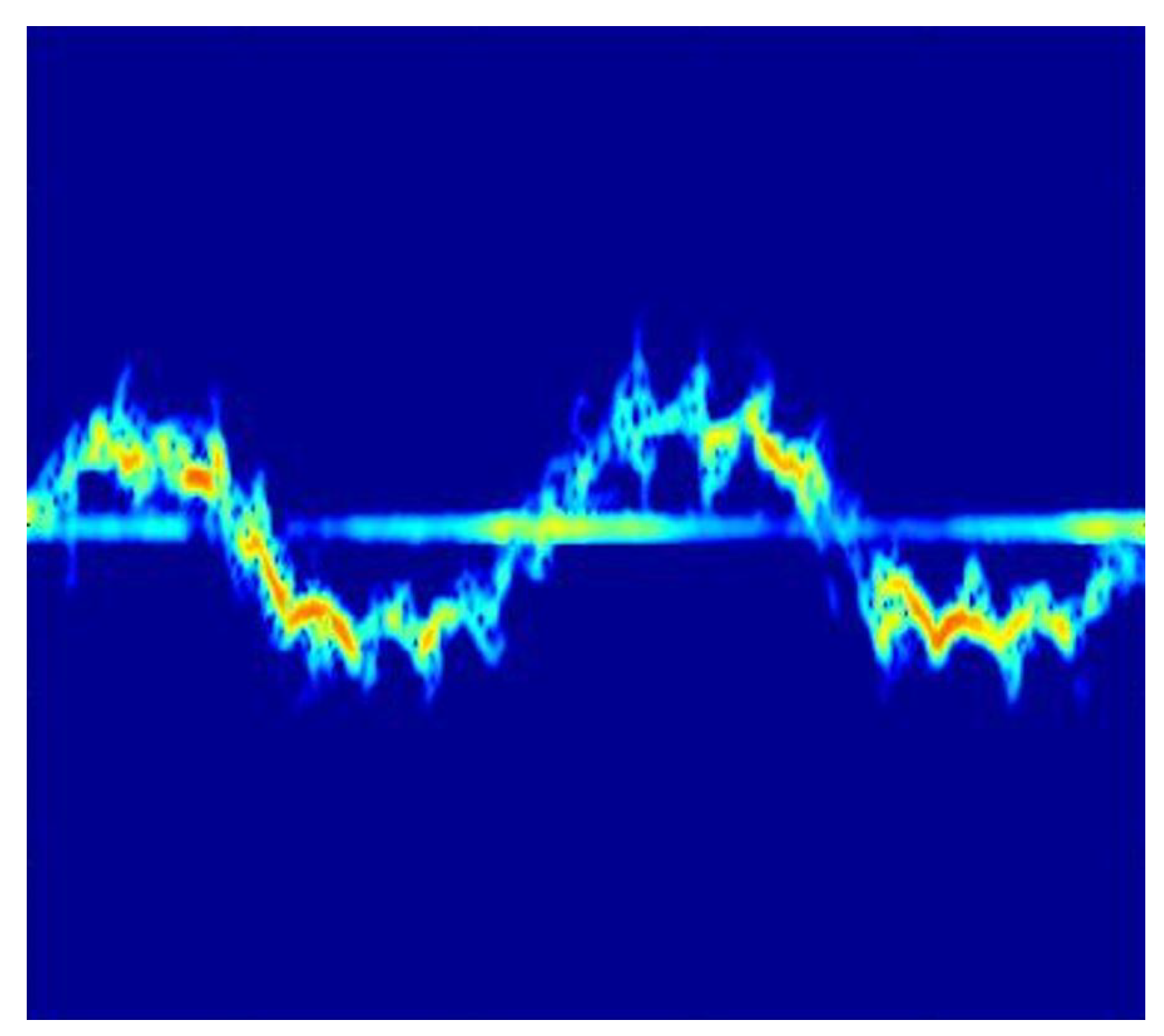
Figure 4.
Data distribution in 3D space and projection onto axes of principal components.
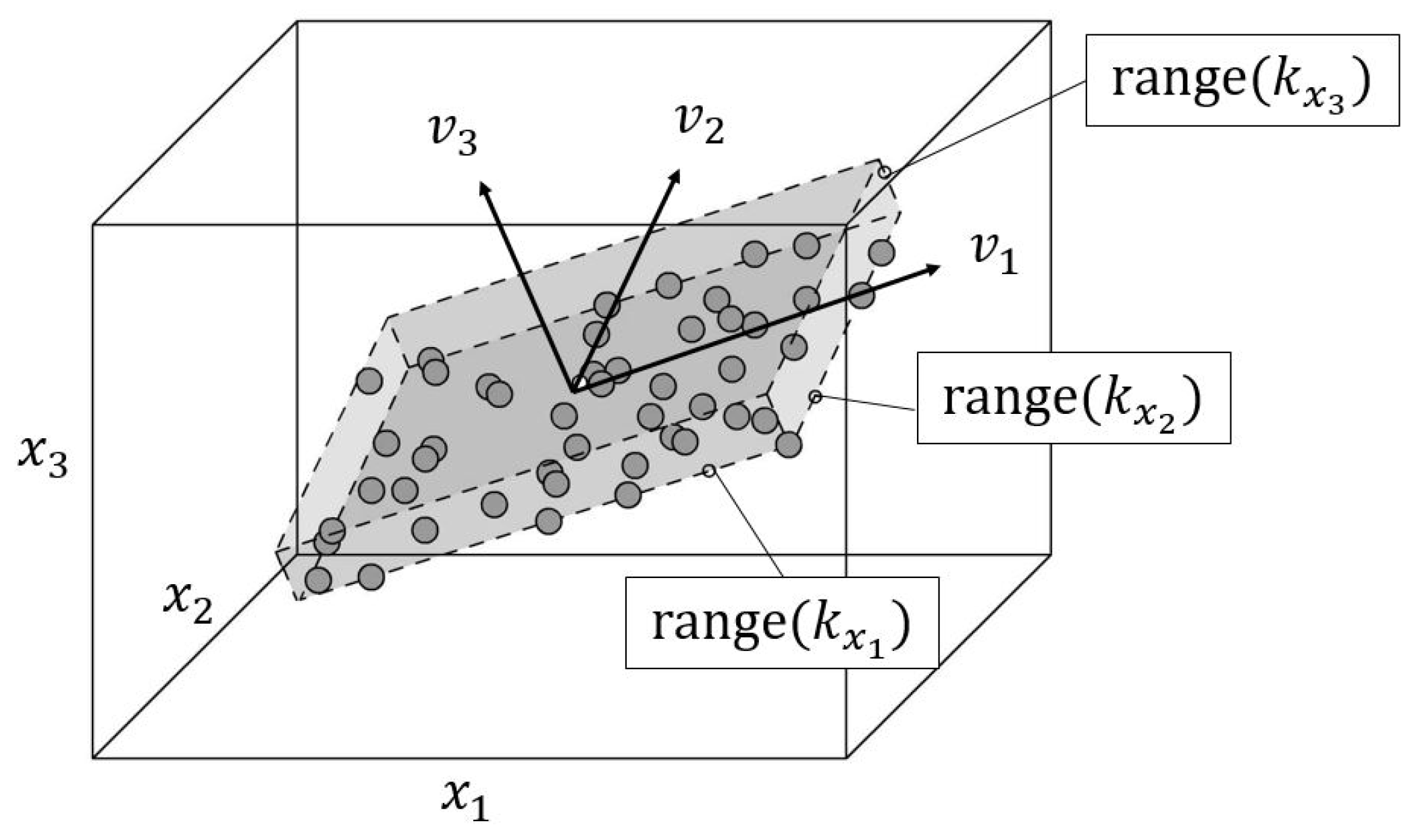
Figure 5.
Convolutional layers.
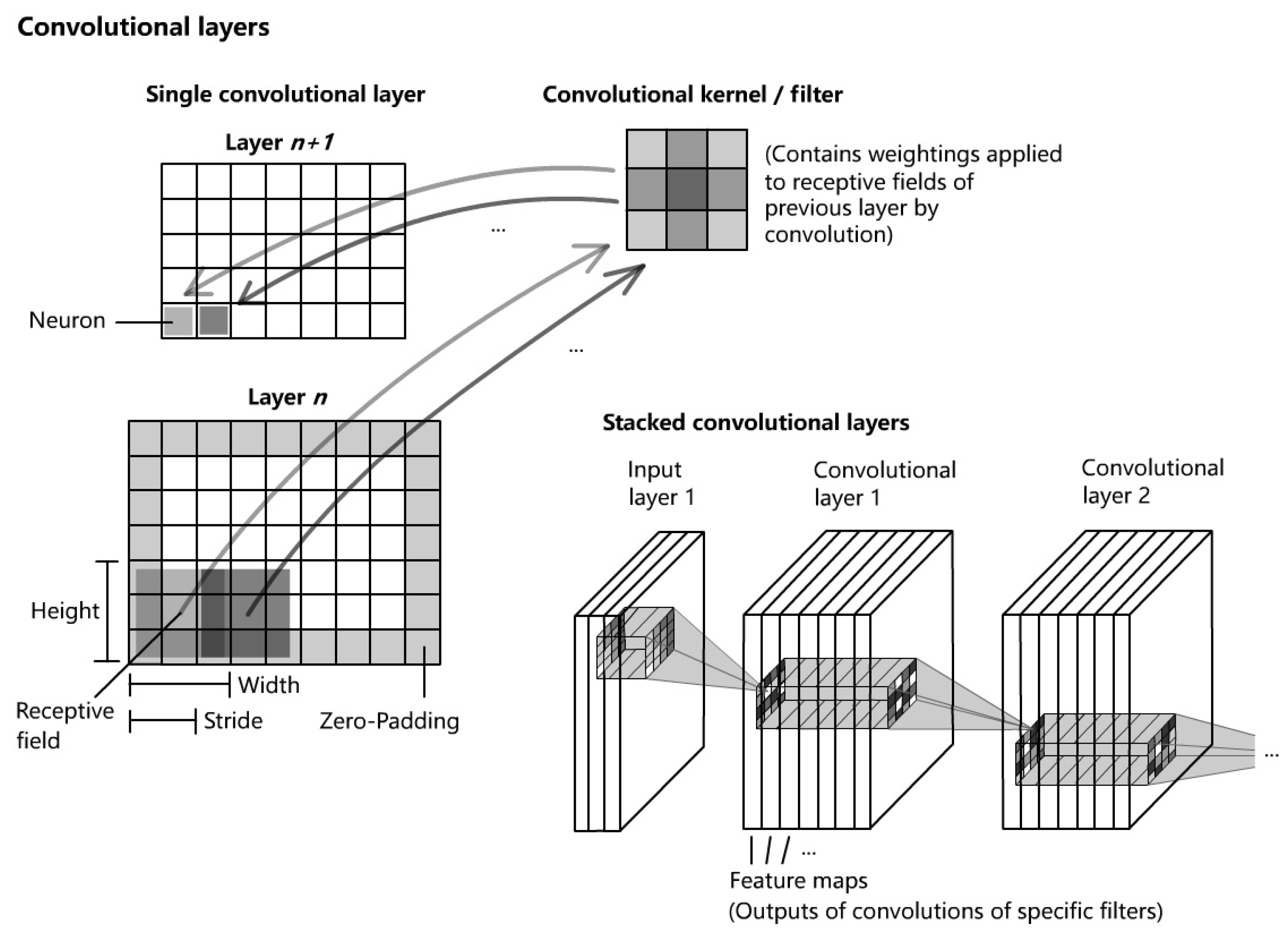
Figure 6.
Stacked RNN: Generalized structure and temporal unrolled variant.
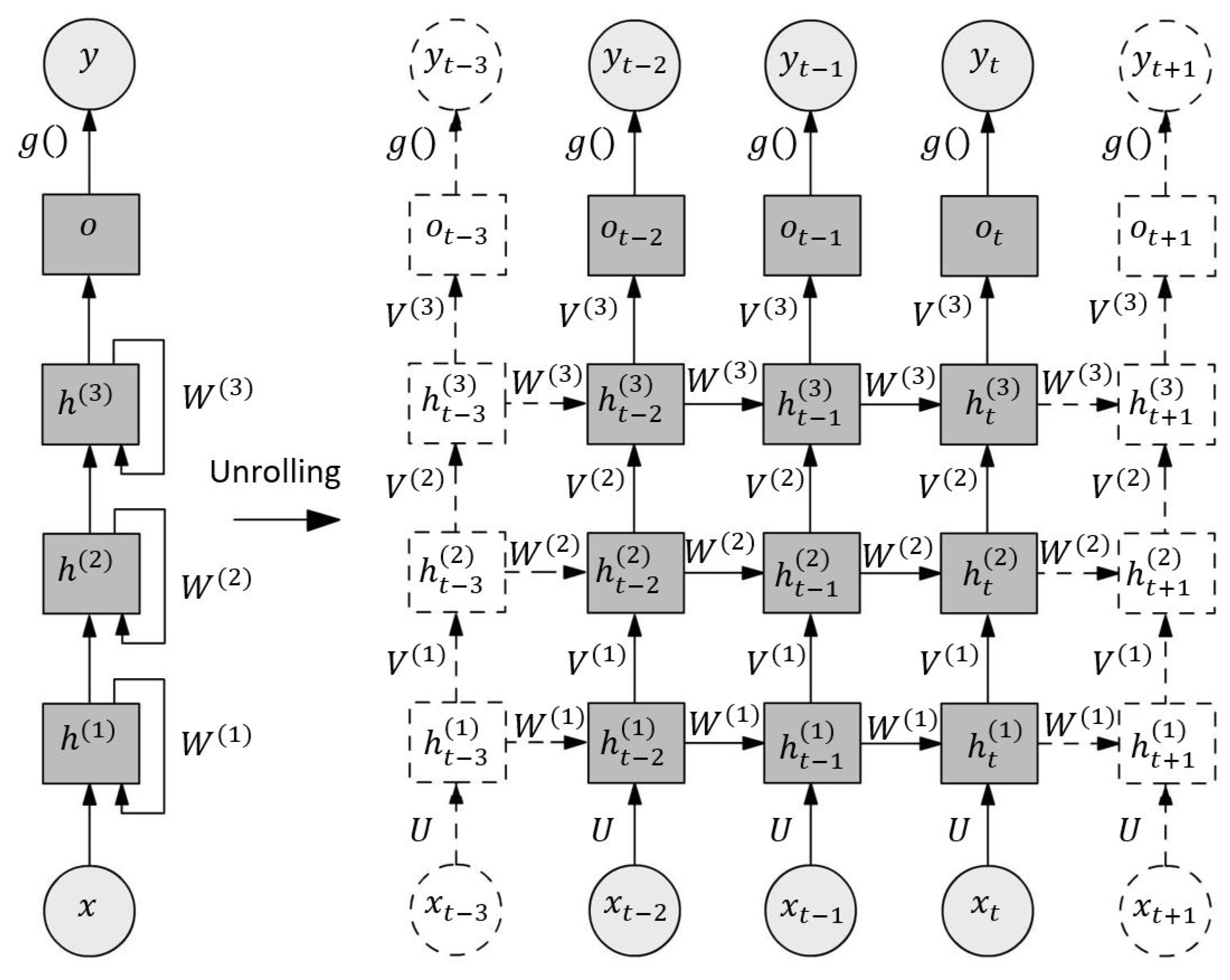
Figure 7.
Standard respresentation of a Peephole Long Short-Term Memory cell.
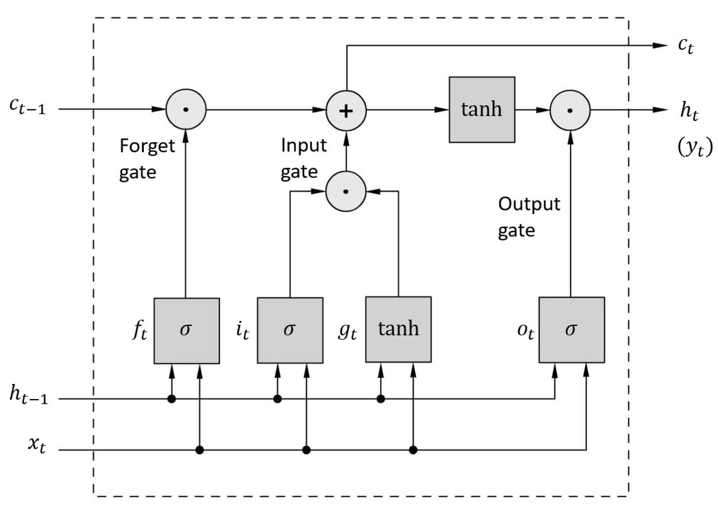
Figure 8.
Example of a stacked autoencoder.
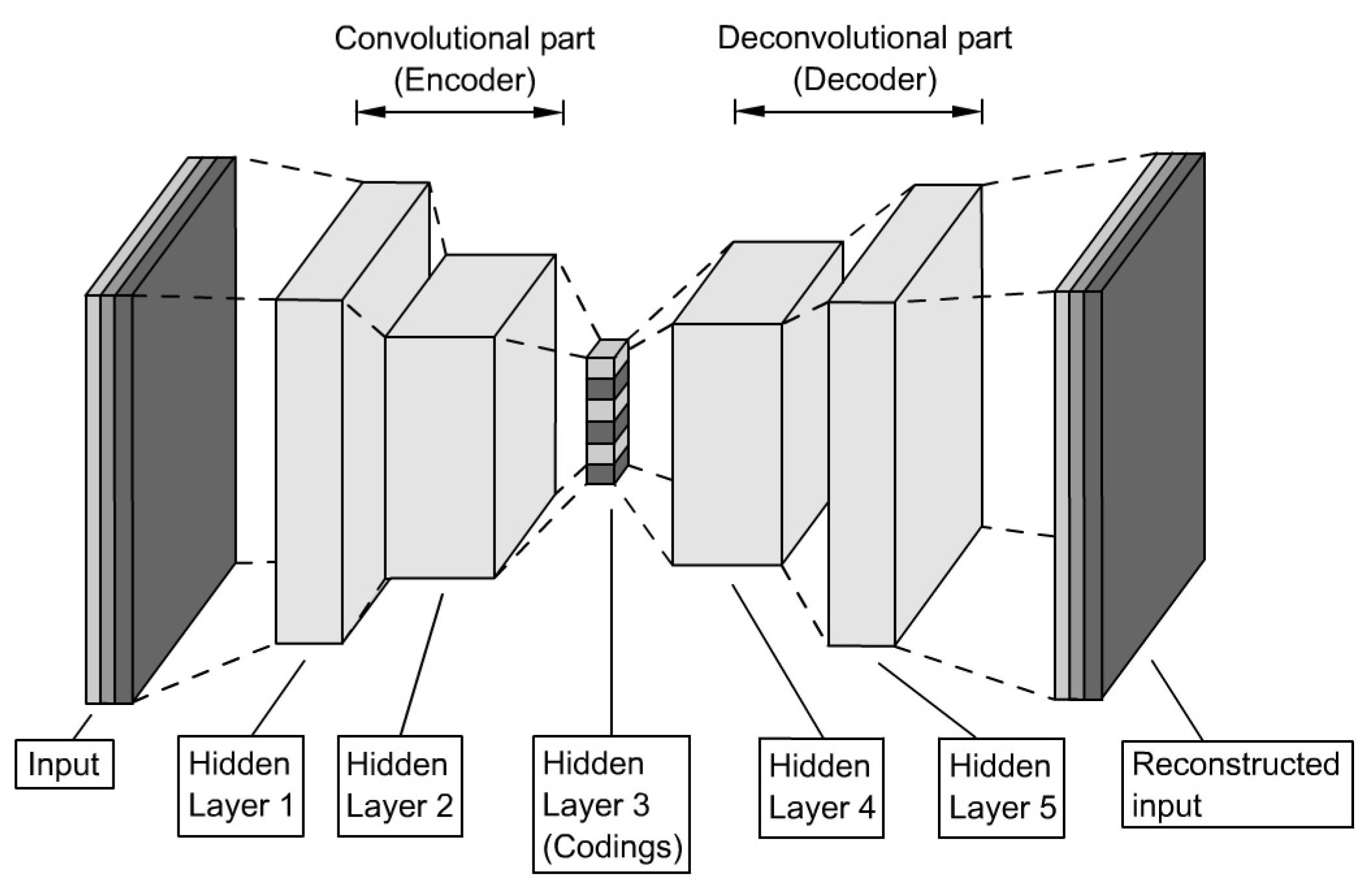
Figure 9.
Example of a Convolutional Autoencoder.
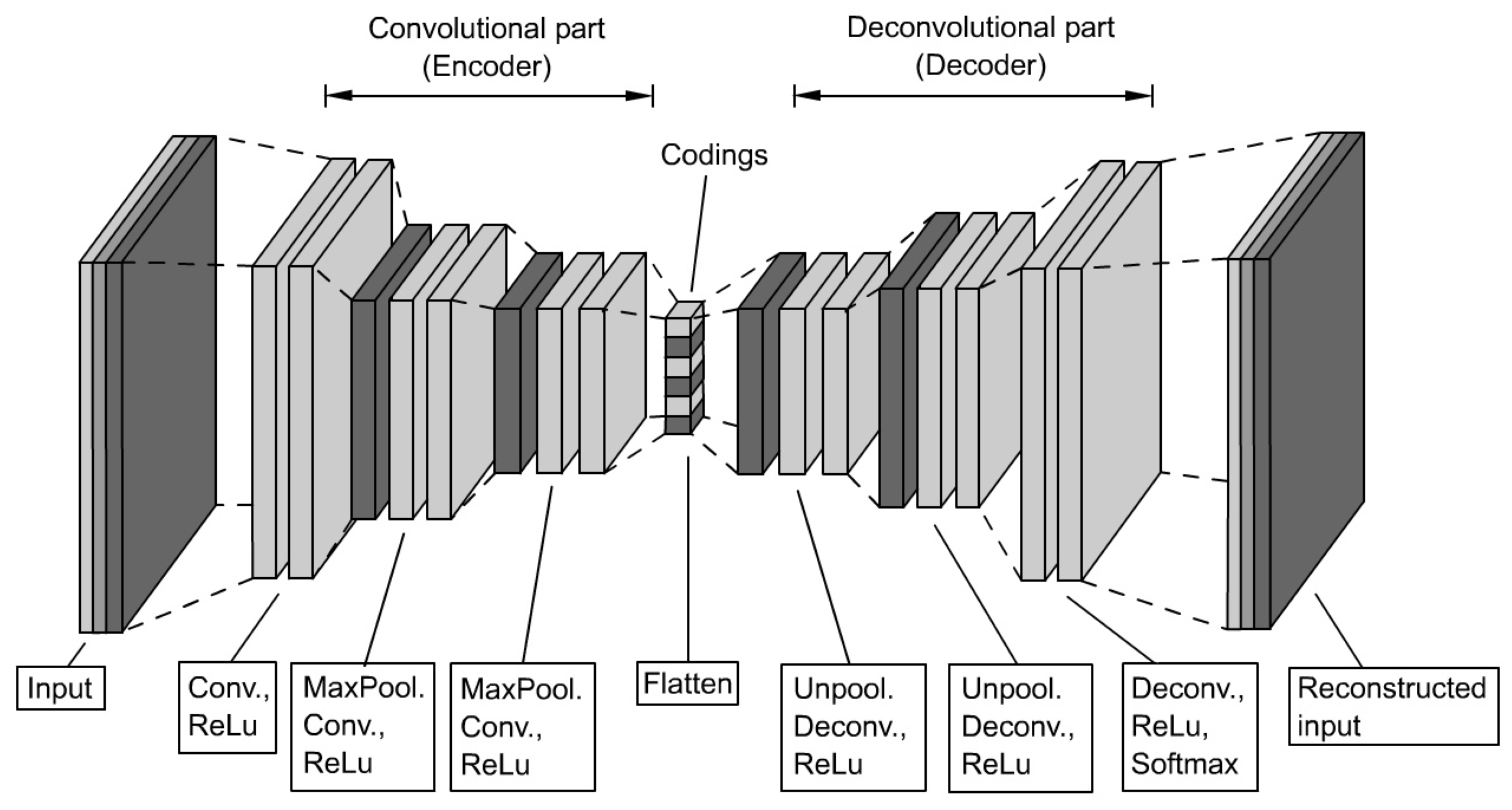
Figure 10.
Unified procedure flowchart.
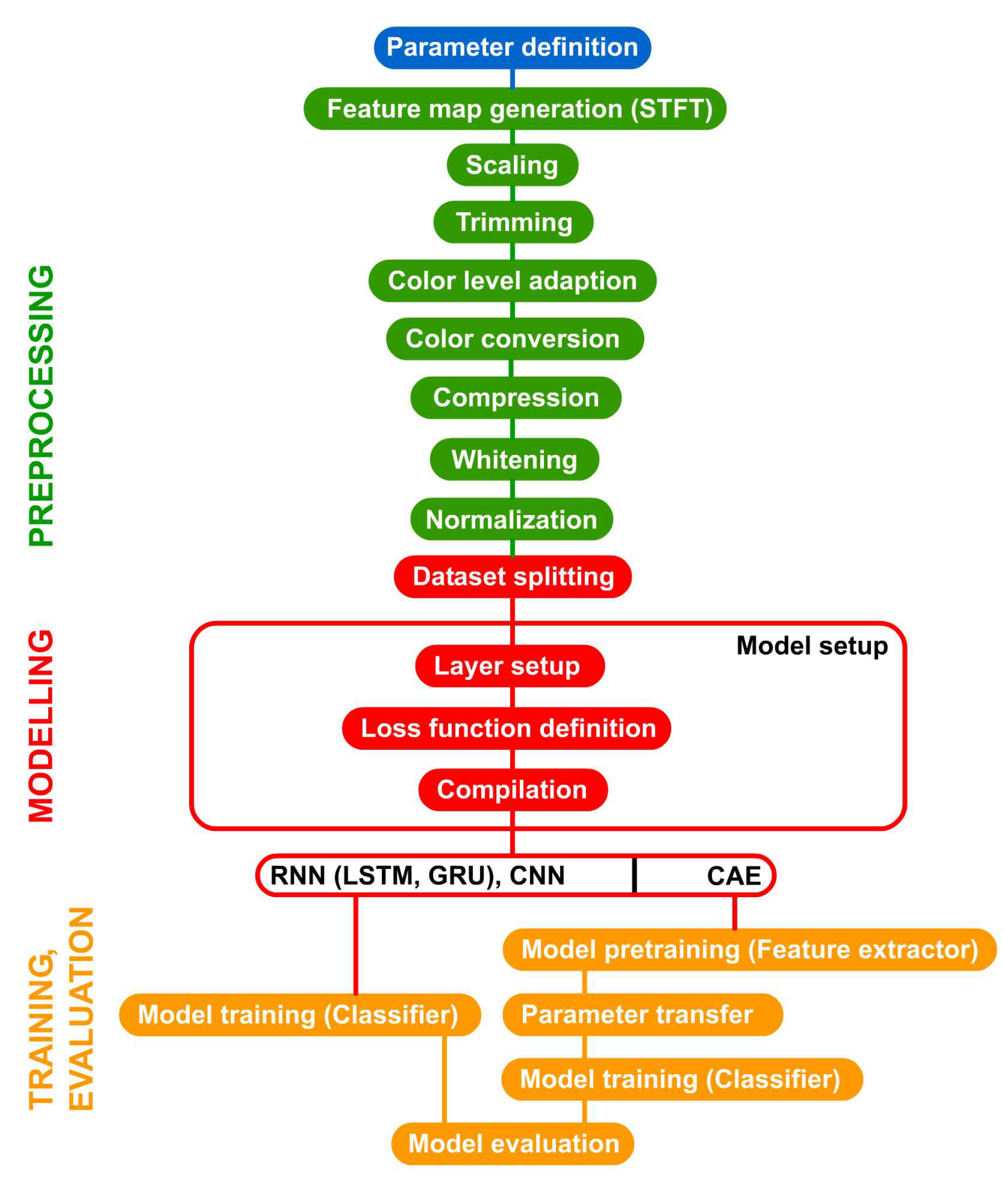
Figure 11.
Images of Micro-Doppler signatures (spectrograms) for six actvities (from [5]).
Figure 11.
Images of Micro-Doppler signatures (spectrograms) for six actvities (from [5]).
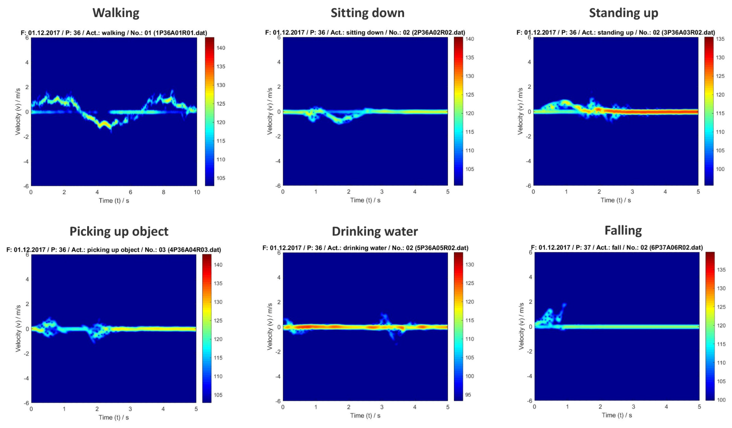
Figure 12.
Selected CNN structure.
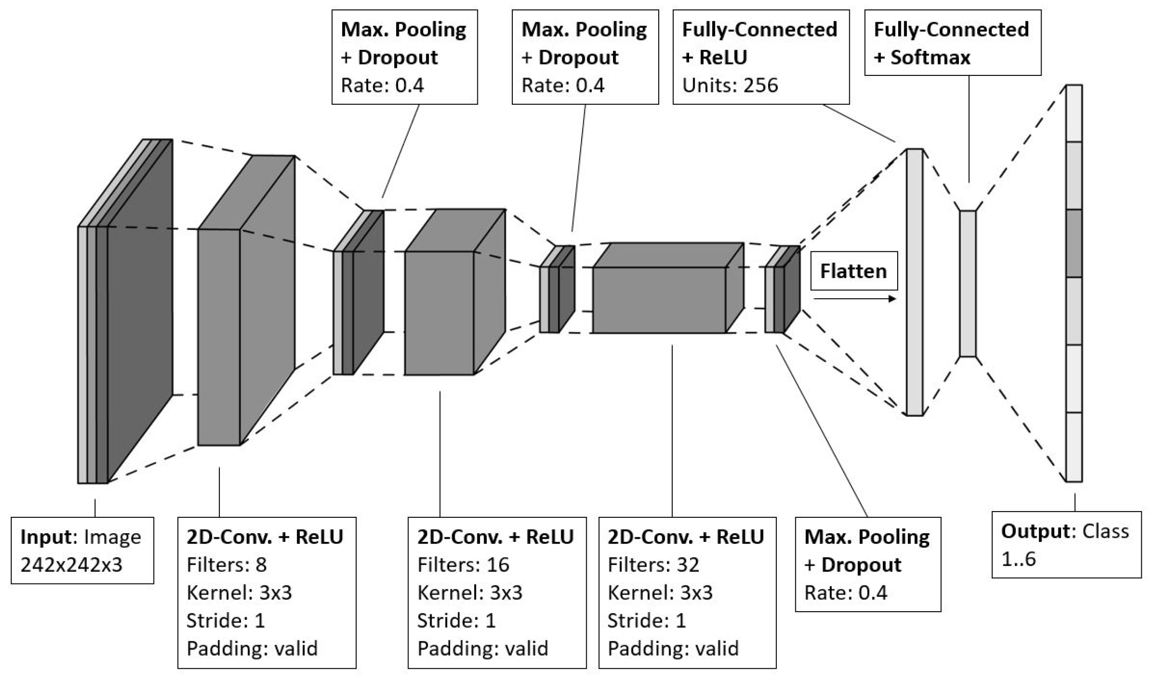
Figure 13.
Selected CAE-based structure.
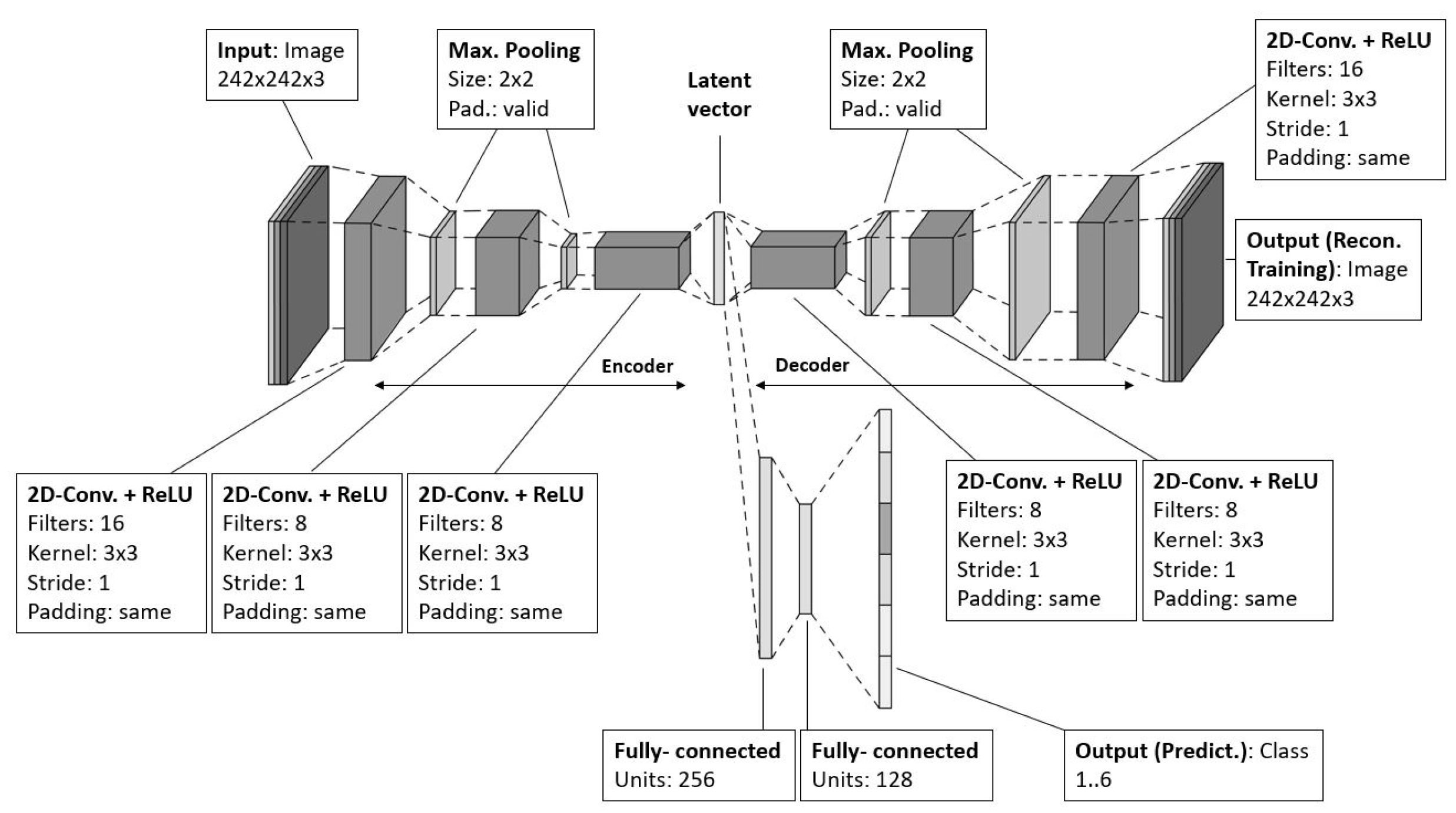
Figure 14.
Loss and accuracy during training and confusion matrix for CNN-based classification.
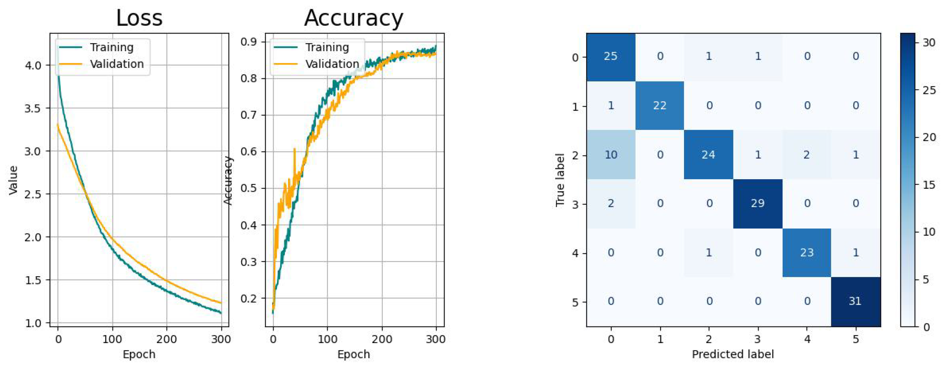
Figure 15.
Loss and accuracy during training and confusion matrix for LSTM(RNN)-based classification.
Figure 15.
Loss and accuracy during training and confusion matrix for LSTM(RNN)-based classification.
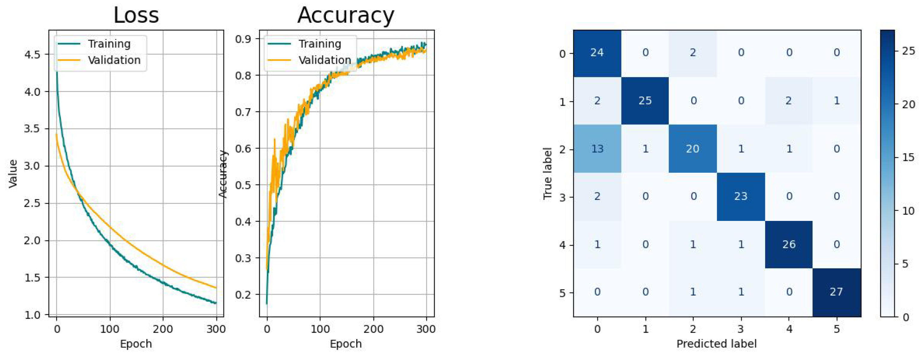
Figure 16.
Loss and accuracy during training and confusion matrix for Bi-LSTM(RNN)-based classification.
Figure 16.
Loss and accuracy during training and confusion matrix for Bi-LSTM(RNN)-based classification.
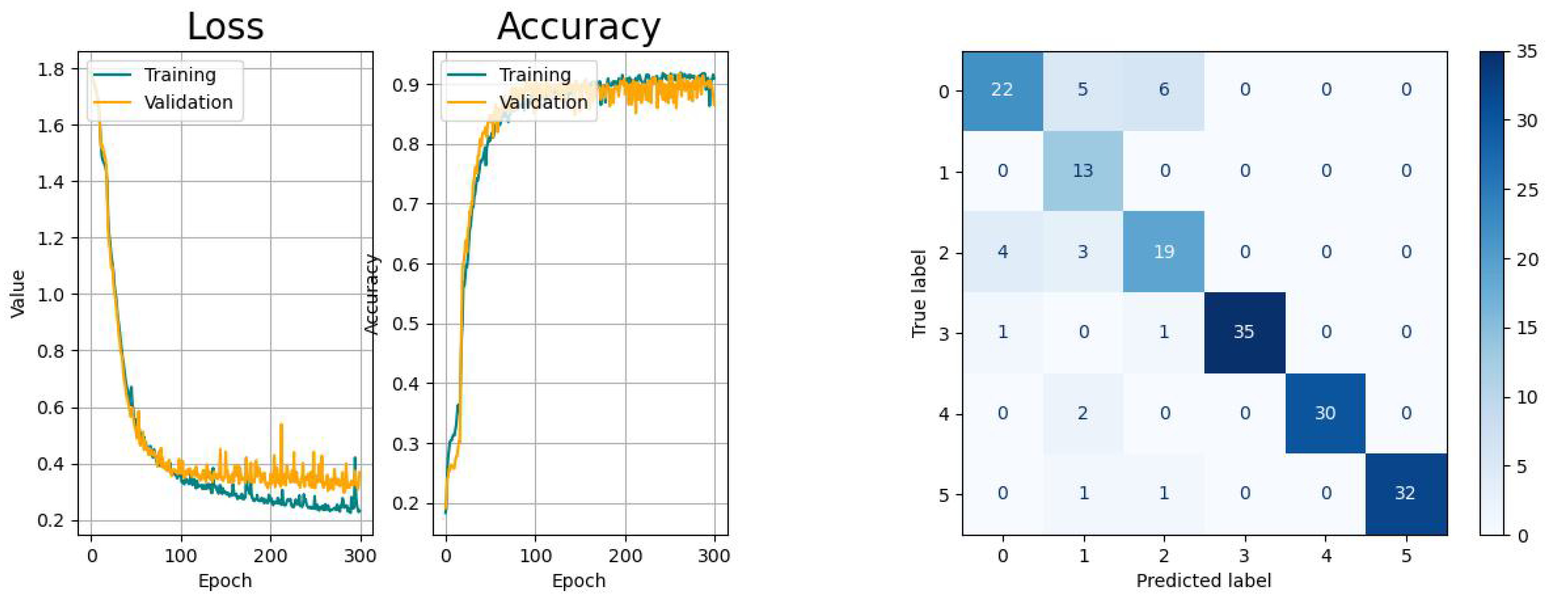
Figure 17.
Loss and accuracy during training and confusion matrix for GRU(RNN)-based classification.
Figure 17.
Loss and accuracy during training and confusion matrix for GRU(RNN)-based classification.
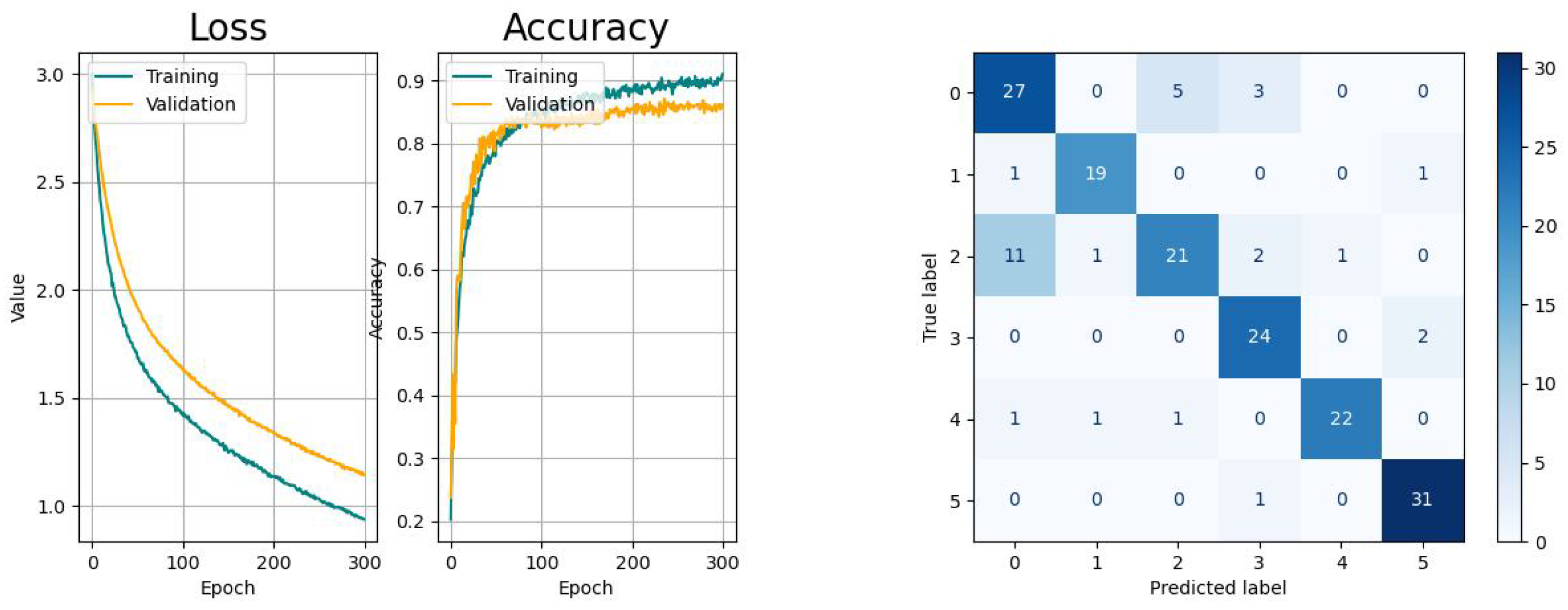
Figure 18.
Loss and accuracy during training and confusion matrix for CAE-based classification.
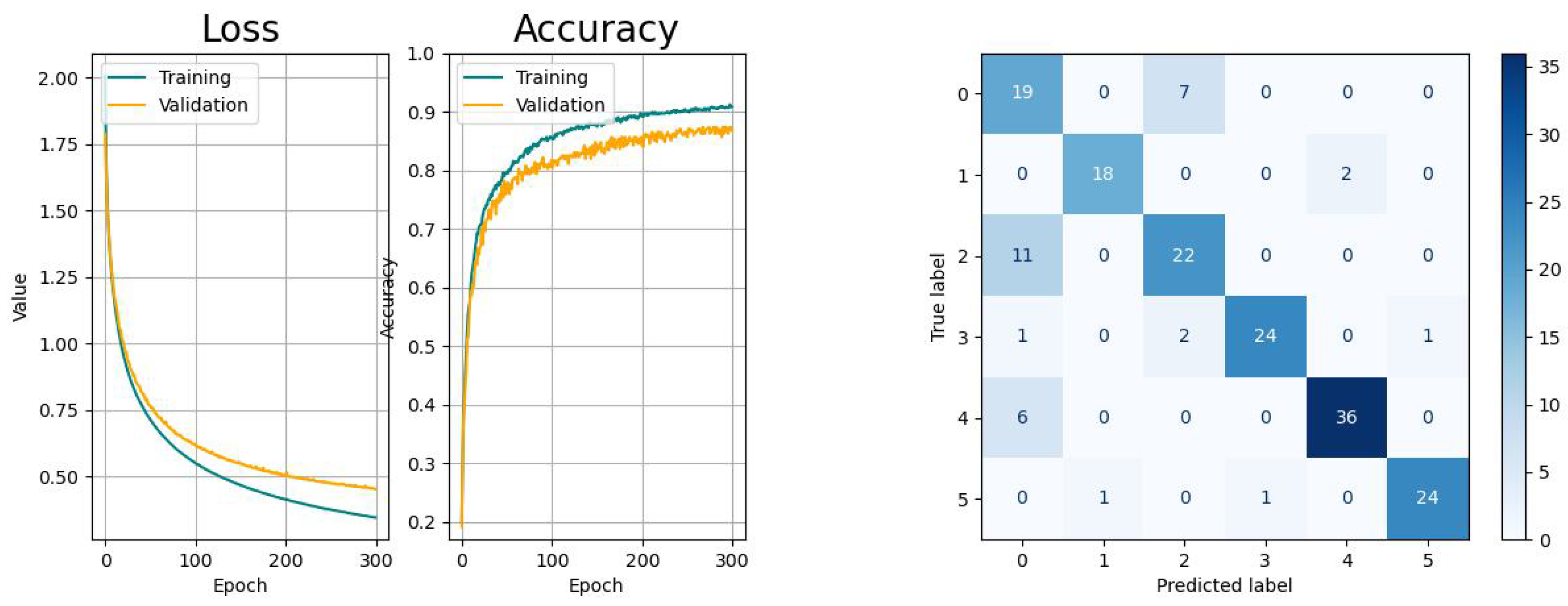
Figure 19.
Accuracy by different lower color value limits used for threshold filtering for the selected models.
Figure 19.
Accuracy by different lower color value limits used for threshold filtering for the selected models.
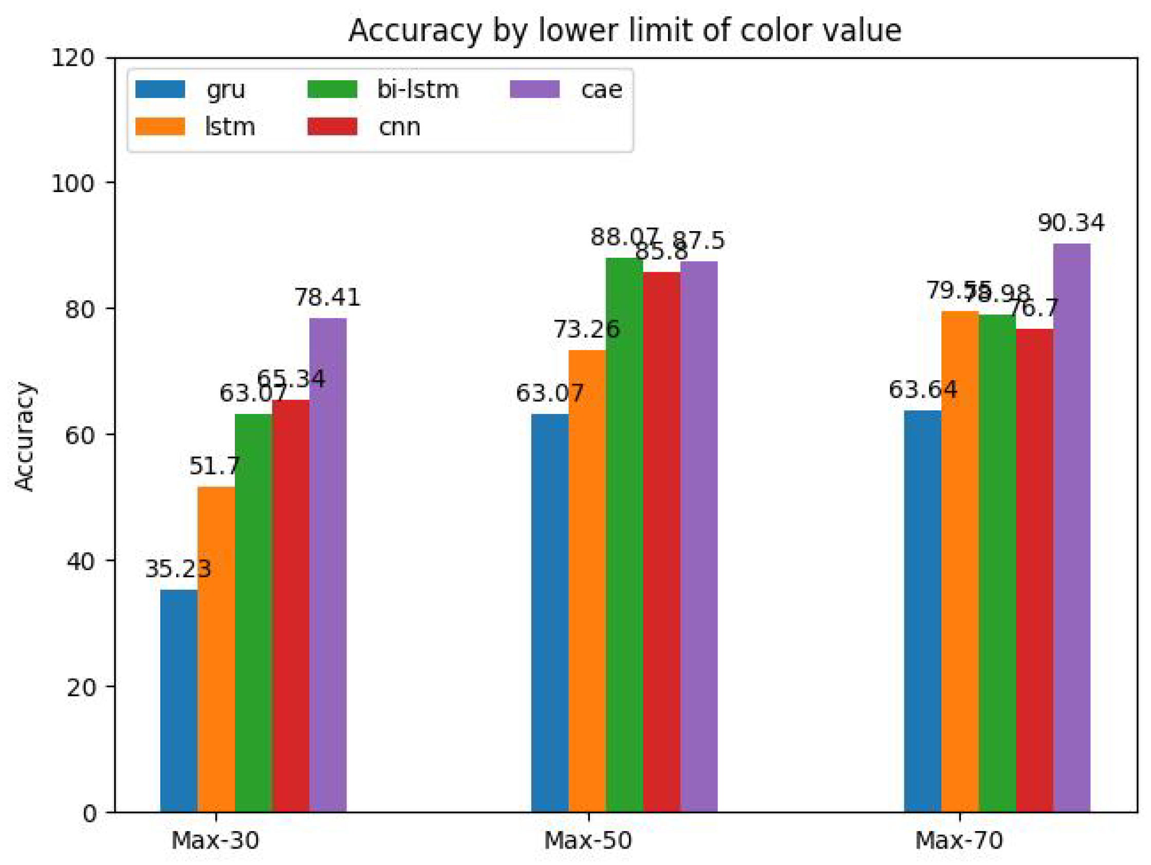
Figure 20.
Accuracy by different compression ratios of the input data for the selected models.
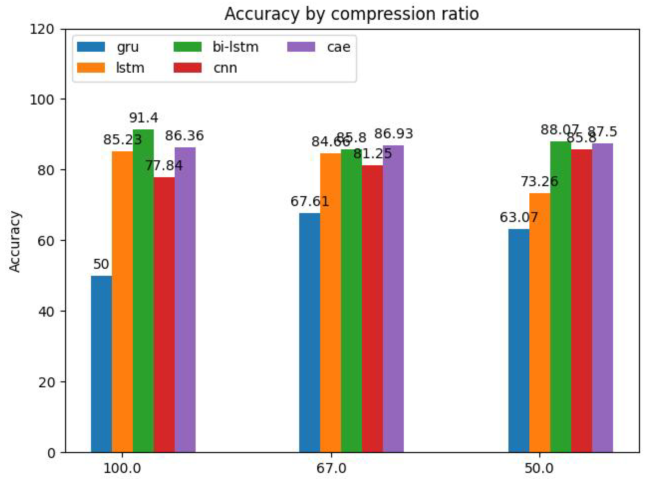
Table 1.
Contents of open dataset radar signatures of human activities [35].
Table 1.
Contents of open dataset radar signatures of human activities [35].
| No. | Date | Number of files | Number of activities | Number of subjects | Number of repetitions |
|---|---|---|---|---|---|
| 1 | Dec. 2017 | 360 | 6 | 20 | 3 |
| 2 | Mar. 2017 | 48 | 6 | 4 | 2 |
| 3 | Jun. 2017 | 162 | 6 | 9 | 3 |
| 4 | Jul. 2018 | 288 | 6 | 16 | 3 |
| 5 | Feb. 2019 | 306 | 6 | 17 | 3 |
| 6 | Feb. 2019 | 301 | 5 | 20 | 3 |
| 7 | Mar. 2019 | 289 | 5 | 20 | 3 |
Table 2.
Number of parameters for the investigated methods.
| Method | Trainable | Non-trainable | Total |
|---|---|---|---|
| CNN | 4,853,174 | 0 | 4,853,174 |
| LSTM | 494,086 | 0 | 494,086 |
| Bi-LSTM | 988,166 | 0 | 988,166 |
| GRU | 371,718 | 0 | 371,718 |
| CAE | 25,691,910 | 94,144 | 25,786,054 |
Table 3.
Performance results and execution time of validation for the investigated methods.
| Method | Accuracy % | Precision % | Recall % | F1 % | MCC % | Cohen Kappa % | Total execution time/s |
|---|---|---|---|---|---|---|---|
| CNN | 88.0 | 89.7 | 88.0 | 87.9 | 86.0 | 91.0 | 3,251 |
| LSTM | 82.3 | 85.6 | 82.9 | 83.0 | 80.1 | 85.5 | 2,966 |
| Bi-LSTM | 86.3 | 88.7 | 86.3 | 86.8 | 83.7 | 90.2 | 10,780 |
| GRU | 82.3 | 82.6 | 82.3 | 82.0 | 78.8 | 86.0 | 2,569 |
| CAE | 81.7 | 84.2 | 81.7 | 82.5 | 78.1 | 78.1 | 7,349 |
Disclaimer/Publisher’s Note: The statements, opinions and data contained in all publications are solely those of the individual author(s) and contributor(s) and not of MDPI and/or the editor(s). MDPI and/or the editor(s) disclaim responsibility for any injury to people or property resulting from any ideas, methods, instructions or products referred to in the content. |
© 2023 by the authors. Licensee MDPI, Basel, Switzerland. This article is an open access article distributed under the terms and conditions of the Creative Commons Attribution (CC BY) license (http://creativecommons.org/licenses/by/4.0/).
Copyright: This open access article is published under a Creative Commons CC BY 4.0 license, which permit the free download, distribution, and reuse, provided that the author and preprint are cited in any reuse.
Submitted:
21 November 2023
Posted:
21 November 2023
You are already at the latest version
Alerts
A peer-reviewed article of this preprint also exists.
This version is not peer-reviewed
Submitted:
21 November 2023
Posted:
21 November 2023
You are already at the latest version
Alerts
Abstract
The importance of radar-based human activity recognition increased significantly over the last two decades in safety and smart surveillance applications due to its superiority towards vision-based sensing in the presence of poor environmental conditions, like illumination, increased radiative heat, occlusion, and fog. An increased public sensitivity for privacy protection, and the progress of cost-effective manufacturing, led to a higher acceptance and distribution. Deep learning approaches proved that the manual feature extraction that relies heavily upon process knowledge can be avoided by its hierarchical, non-descriptive nature. On the other hand, ML techniques based on manual feature extraction provide a robust, yet empirical based approach where the computational effort is comparatively low. This review outlines the basics of classical ML- and DL-based human activity recognition and its advances while taking recent progress of both categories into regard. For every category, state-of-the-art methods are introduced, briefly explained and discussed in terms of their pros, cons and gaps. A comparative study is performed to evaluate the performance and computational effort based on a benchmarking data set to provide a common basis for the assessment of the techniques’ degree of suitability.
Keywords:
Subject: Computer Science and Mathematics - Artificial Intelligence and Machine Learning
1. Introduction
In the last two decades, civil radar-based applications, as they are used for human sensing and human activity recognition (HAR), have made significant progress. This has been triggered and supported by the rapid development in semiconductor technologies in recent decades, in particular by the drastic change in the concept of radar. Modern radar systems are highly integrated, i.e. the most important circuits are housed on a single chip or a small circuit board.
The potential of radar-based sensing and recognition technologies has been discovered by a variety of different scientific domains and was the target of numerous preceding and recent research. First studies dealt with the detection of humans and recognition in indoor environments for application regarding security [1,2,3,4,5,6]. Medical applications, i.e. monitoring of patients extended its applicability [7,8,9,10,11,12,13] to sub-domains, e.g. vital sign detection. In addition, the latest developments of autonomous driving have impressively shown the enormous potential of radar-based automotive human activity and security applications, e.g. gesture recognition [14,15,16,17,18,19,20,21,22,23,24,25] and safety-oriented car assistance systems, e.g. fatigue recognition [26] or occupant detection [27,28,29,30,31,32], especially of forgotten rear-seated or wrongly placed infants or children, in order to prevent deaths due to overheating or overpowered airbags. In comparison to the aforementioned application field, automotive-specific applications suffer excessively by different environmental conditions due to the variation of light, temperature, humidity and occlusion. Further, increasing demands for privacy-compliant smart home solutions, e.g. for the intelligent control of heating [20] or the surveillance of elderly people in order to detect falls [9], have led to an unprecedented technological pace.
Although the advantages of vision-based sensing and recognition technologies are undisputed, there are many situations, where the drawbacks are severe, compared to radar-based technologies. Sensing-related problems comprise lighting conditions (poor illumination), thermal conditions (increased radiative heat), occlusion and atmospheric phenomena (fog, mirage). Besides those, radar-based systems are independent of privacy-related conditions, since target information do not rely explicitly on target shapes, but can be derived of microscale movements based on Micro-Doppler signatures [33,34,35,36,37,38].
The radar-based recognition of human activities has been studied by numerous authors, where classical Machine-Learning (ML) based techniques, e.g. k-Means [39], SVM [40,41,42,43,44] etc. as well as Deep Learning-based (DL) approaches have been used [45,46,47,48,49,50,51,52,53,54,55,56,57,58,59,60,61,62,63,64,65,66,67,68,69,70]. In general, ML-based techniques rely on shallow heuristically determined features that are characterized by simple statistical properties and thus, depend on technological experience. Furthermore, the learning process is restricted to static data and does not take long-term changes of the process data into consideration.
Deep Learning constitutes a subdomain of Machine Learning, where the methods applicability do not depend on the suitability of hand-crafted features. Feature extraction highly relies on domain knowledge and the the expertise of the user in particular. Instead, the deep learning approaches are able to extract high-level, yet not fully interpretable information in a generalized approach, and due to their structure, the underlying learning process can be designed to increase computational efficiency, e.g. by parallelization.
This work addresses the recent progress of ML-based HAR methods in radar technology setting and focuses on DL-based approaches, since those have proven to be a more generalized, long-term oriented, and robust solutions for classification problems. One major contribution of this paper is to provide the first comparative study of HAR methods using a common data base and a unified approach for the application of the most common DL methods while focussing on key aspects: CNN-, RNN- and CAE-based methods. The goal is to investigate the performance associated with computational cost, i.e. the total execution time and the space complexity, i.e. the parametricity of those methods under equal conditions in order to determine the suitability through comparison from which general recommendations can be derived. Furthermore, a unified approach for the classification task using different methods but a common preprocessing is proposed. The importance of careful preprocessing of the input data is provided by two variational studies. In the first study, the lower color value limit of the derived feature maps is varied and the impact on the accuracy is evaluated. This is important, since the characteristic patterns rely strongly on the color range, where high thresholds are associated with a higher degree of loss of important information, while low thresholds may contain redundant information, which, regardless of the model, could increase the risk of overfitting. In the second study, the impact of data compression of the feature maps on the accuracy is evaluated, since data reduction leads to lower storage requirements and hence reduced costs for hardware or faster data transmission rates for online systems.
The remaining sections are organized as follows: In Section 2, the basic principles of radar are outlined and briefly explained. Then, common preprocessing techniques are presented in Section 3, whereas Section 4 emphasizes on the recent progress of DL-based approaches after giving a short introduction. In Section 5, a comparative study of the most successful approaches and state-of-the-art methods of both preceding sections based on benchmark data are provided, where the performance, computational effort and the space complexity is evaluated and discussed in Section 6. Finally, the paper closes by presenting open research topics, derived by current gaps and challenging issues of the future.
2. Basic Principles
2.1. Radar-based Sensing
The underlying principle of the radar-based detection of targets, in general, is to emit and to receive electromagnetic waves (RF signals), which contain information about the targets properties. A common categorization of radar systems is to classify them into systems based on pulse radar or continuous wave. Both categories have their individual applications with specific advantages and disadvantages with regard to distance resolution, velocity resolution, power consumption, technical equipment, waveform generation, signal processing, etc.
2.2. Continuous Wave Radar
The main characteristic of Continuous Wave Radar systems (CW) is to emit a continuous electromagnetic wave using a sine-waveform, where the amplitude and frequency remains constant and to process the wave reflected by the target. Besides information about the reflectability, it contains information about the target’s velocity due to the Doppler frequency shift. A common variant of this technique are FMCW radar systems, whose waveform vary in the time-domain.
With regard to HAR, FMCW-based radar systems in the mm-wave domain have significant advantages compared to CW radar as the suitability for human sensing has been proven by numerous works in the last two decades [40,41,42,46,48,50,57]:
- High sensitivity: For the detection of human motions, especially for the small-scale motions, e.g. like breathing and gestures, a sensitivity close to the wavelength is required. This can be achieved when a high center frequency combined with a high bandwidth (B) is used.
- Minimized danger of multipath propagation and interactions with nearby radar systems due to the high attenuation of the mm-wave RF signal
- Distances and velocities of targets can be measured simultaneously, e.g. when triangular modulation of the chirp signal combined with a related signal processing technique is used.
- Independence to thermal noise as the phase is the main carrier containing information about targets distances
Figure 1.
Schematic representation of a FMCW-based radar sensor.
FMCW radar generate a sinusoidal power-amplified RF signal (chirp) by a high-frequency oscillating unit, where the frequency is varied linearly between two values and in sawtooth-like pattern over a certain duration according to the following function:
Figure 2.
Time-related characteristics of the chirp signal with sawtooth and triangular shape modulation.
Figure 2.
Time-related characteristics of the chirp signal with sawtooth and triangular shape modulation.
The constant / for determines the slope of generated signal, whereas the frequency variation is determined by a linear function. This RF signal is emitted via the transmitting antenna and the echo signal, which follows from the scattered reflection of the electromagnetic waves on the objects, are received at the receiving antenna and low noise-amplified. A mixer processes both, the transmitted and received signal, and generates a low-frequent beat signal, which, in the following, is preprocessed and used for the analysis.
A linear chirp signal that can be defined within the interval by
is emitted and mixed with its received echo signal to provide the IF signal
which, in the following, is preprocessed and used for the calculation of the feature maps.
In general, human large-scale kinematics, e.g. the bipedal gait, are characterized by complex interconnected movements, mainly of the body and the limbs. While the limbs have oscillating velocity patterns, the torso can be characterized by transitional movement solely.
According to the Doppler effect, moving rigid-body targets induce a frequency shift in the carrier signal of coherent radar systems that is determined in its simplest form by
where v is the relative velocity between the source and the target and the frequency of the transmitted signal. While the torso induces more or less constant Doppler frequency shifts, the limbs produce oscillating sidebands, which are referred to as micro-Doppler signatures [33]. In the joint time-frequency plane, these micro-Doppler signatures have distinguishable patterns, which make them suitable for ML-based classification applications. An example of can be found in Figure 3.
Micro-Doppler signatures are derived by time-dependent frequency-domain transformations. The first step is to transform the raw data of the beat signal to a time-dependent range distribution, referred to as the time-range distribution by the fast Fourier transform (FFT), where m is the range index and n the slow time index (time index along chirps).
While the Fourier-transformation is unable to calculate the time-dependent spectral distribution of the signal, the short-time Fourier transform (STFT) is a widely used method for the linear time-varying analysis that provides a joint time-frequency plane. In the time-discrete domain, it is defined by the sum of the signal values multiplied with a window-function, which is typically the Gaussian function to provide the Gabor transform:
Applied to the time-range distribution matrix , the time-discrete STFT can be computed by:
The spectrogram, also referred to as Time-Doppler Spectrogram (DT), is derived from the squared magnitude of the STFT:
Besides the STFT of the time-range distribution matrix, a FFT using a sliding window along the slow time dimension obtains time-specific transformation in the time-frequency domain, which are called range-Doppler distributions (RD).
A modification of the FMCW radar is the Chirp Sequence Radar [71]. It facilitates the unambiguous measurement of range R and relative velocity simultaneously, even in the presence of multiple targets. To do this, fast chirps of short duration are applied. The beat signals are processed in a twodimensional FFT to provide measurement of both variables by frequency measurements in the time domain t and the short-time domain k instead of a frequency and phase measurement, as it is the case for the regular FMCW radar. This method reduces the correlation between range and relative velocity and improves the overall accuracy.
2.3. Pulse radar
While the CW-based radar and its subclasses rely on moving targets to create micro-Doppler signatures, pulse radar is able to gather range information of non-moving targets, e.g. human postures by applying short electromagnetic pulses. A modification, which combines principles from both, CW and pulse radar, is pulse-Doppler radar.
In pulse radar, the RF signal is generated by turning on the emitter for a short period of time while switching to the receiver after turning of the emitter and listening for the reflection. The measuring principle is based on the determination of the round-trip time of the RF signal, which has to meet specific requirements with regard to the maximum range and range resolution that are determined by the pulse repetition frequency (PRF) or, alternatively, the interpulse period (IPP) and the pulse width (), respectively. A variant of pulse radar is Ultra-Wideband (UWB) radar, which is characterized by low-powered signals and very short pulse widths, which leads to a more precise range determination while having a drawback with regard to the Signal-to-Noise Ratio (SNR).
The reflected RF signals contain intercorrelated information about the target and its components, i.e. human limbs as well as the surrounding environments by scattering effects in conjunction with multipath propagation. Due its high resolution, small changes in human postures create different measurable changes in the shape of the reflected signal. Using sequences of preprocessed pulse signatures, specific activities can be distinguished between each other and used as features for the setup of classification models.
In [70], the authors developed and investigated a time-modulated UWB radar system to detect adult humans inside a building for security purposes. In contrast to static detection, [44] used the a bistatic UWB radar to collect data of eight coarse-grained activities for human activity classification. The data were collected at the center frequency of 4.7 GHz with a resolution bandwidth (RBW) of 3.2 GHz and a RBF of 9.6 MHz, which were reduced in dimensionality by the Principal Component Analysis (will be explained in the next chapter) and used within a classification task based on Support Vector Machine (SVM) after a manual feature extraction using the histogram of principal components for a short time window.
2.4. Preprocessing
In general, returned radio signals suffer from external incoherent influences, i.e. clutter and noise, and are therefore unsuitable for the training of machine-learning based classification methods. In addition to this aspect concerning the data quality, the success as well as the performance of classification methods depends on the data representation, the data dimensionality and the information density. Thus, it is necessary to apply signal processing techniques in order to enhance the data properties prior to the training and classification. The next subsection give a brief description of settled preprocessing methods.
2.4.1. Clutter
Radio signals reflected by the ground lead to a deterioration of data quality in general as it contains information unrelated to the object or the task. The difficulty for the determination and removal depends strongly on the situational conditions.
In static environments, the clutter can be removed by simply subtracting the data containing the relevant object from the data that were collected previously, where the object was missing [44]. Nevertheless, quasi-static or dynamic environments are characterized by changing conditions as they occur for mobile applications, storage areas etc. can affect the data.
Numerous works that emerged in the latest years, based their work on different approaches, e.g. sophisticated filters using eigenimages derived by Singular Value Decomposition (SVD) for filtering, combinations between Principal Component Analysis (which will be explained in Subsection E) as well as filtering in the wavenumber domain using predictive deconvolution, Radon transform or f-k filtering [74,75].
2.4.2. Denoising
One of the major problems for machine learning applications is called overfitting. It occurs when the model has a much higher complexity or degree of freedom with regard to the input data that was used for training. It leads to a perfect fitting to the training data but fails when other data, i.e. for testing, are considered.
To overcome this lack of generalization, when other factors can be excluded (e.g. the amount of data is sufficient), denoising is one the techniques to improve the accuracy. Using Low-pass filters, convolutional filters or model-based filters are the most common methods to reduce noise, which may mislead the algorithm to learn patterns that do not refer to the process itself.
Apart from that, adding noise may increase the robustness. In [61], Denoising Autoencoders (DAE) are used, where noise is added to the input data that leads to an overall increase of the models generalization ability. The most common method is to add isotropic Gaussian noise to the input data [62]. Another way is to apply masking noise or salt-and-pepper-noise, which means that a certain fraction of the input data is set to zero or changed to its corresponding maximum or minimum value, respectively [62].
2.4.3. Normalization
As the amplitudes of the target signatures depend substantially on the distance between sensor and the target, the normalization of the data is required in order to maintain consistent statistical properties, e.g uniform SNR, which are required for the training of ML models.
2.4.4. Data Reduction
The Principal Component Analysis (PCA) is a common method used for the reduction of the data dimensionality, which is beneficial for algorithms to learn efficiently [40]. Its main idea is to preserve the maximum variance of the data while projecting them onto a lower dimensional hyperplane using the first eigenvectors, called the principal components, where every predominant subset of principal components defines a plane, which is orthogonal to the following principal component (see Figure 4).
Due to its increased numerical stability, the Singular Value Decomposition (SVD) is a typical method for the calculation of the principal components :
To obtain a reduced dataset, the first m principal components, where the cumulated explained variance ratio exceeds a certain target threshold, are selected to form a matrix, which is multiplied by the original data matrix:
2.4.5. Whitening
Closely related to the normalization, whitening refers to a more generalized method, where a transformation is applied to input data so that the diagonal elements of the covariance matrix are all ones (also called sphering). This method reduces the correlation between the input data and improves the efficiency of the learning algorithm. The most common methods in connection with that are the Principal component analysis (PCA), the Zero-Phase Component Analysis Whitening (ZCA) and the Cholesky Decomposition [72,73].
The Prinicipal Component Analysis is the most popular procedure for decorrelating data, which can be used to reduce the dimensionality of data while the variance of data is maximized. With regard to twodimensional data structures, like e.g. images, this is achieved by determining the covariance matrix, which is decomposed using the SVD into two orthogonal matrices and one diagonal matrix , where the diagonal matrix contains the eigenvalues. Taking only the first n components of the eigenvector matrix along with their corresponding eigenvalues it is possible to obtain a compressed version of the original image. Here, it is used to compute the conversion matrix , which can be multiplied with the original matrix to achieve decorrelation:
The small constant , which is usually around is inserted to avoid large coefficients that are caused by the reciprocal of very small eigenvalues. The zero-phase transformation
is a whitening procedure, where the transformation leads to uncorrelated data with, in contrast to the PCA, unit variances and is computed using the PCA and an additional multiplication with the eigenvector matrix .
2.5. Feature Engineering
In general, the selection and extraction of features during feature engineering is crucial for the success of machine learning applications. The term selection refers to the identification of strongly influencing measurable properties with regard to the mathematical task while extraction deals with the dimensionality reduction when using compositions of features. For example, in [40], the PCA is used to determine the histogram of the most influencing PC for given time window, from which the mean and variance are used as features. Another example is [37], where the number of discrete frequency components are determined using spectrograms that contain micro-Doppler signatures, which provides useful information about the location of small-scale motions.
Classical techniques, e.g. Linear Regression, Decision Trees, Random Forests, k-Nearest Neighbor, etc. rely heavily on handcrafted feature engineering, which implies a certain experience and domain-knowledge, while DL methods use algorithms that select useful features automatically, which, as a main drawback are hardly interpretable by humans and indirectly evaluable.
2.6. Challenges
Besides the numerous convincing applications of machine-learning methods to human activity recognition, there are still topics that haven’t been investigated yet or at least, have only been partially addressed. In general, these challenges can be divided into source-related problems and methodological problems that are presented in the following subsections.
The first source-related problem deals with the fact that related works pursue different aspects of human activity recognition and rely on own data acquisition, which is depending on the activities the authors focus. Different data sets with varying activities of different scale constitute a major problem, as the condition for comparability is simply not given, e.g. [40,41,42,48,50,53,57,59] use coarse-grained activities for their investigation while [26,46] use fine-grained activities as a basis for their works. Especially, the last point states a problem, since the movements are linked to weaker micro-Doppler signatures in terms of power.
Another problem is that many activities of both degrees of fineness classes have a certain similarity, which has been proven, e.g. by [40], where data collected from coarse-grained activities were used for a SVM-base binary classification problem and activities like punching were confused with running.
Among other factors, every activity has its unique micro-Doppler signature, so machine learning-based classification models are trained to distinguish between the specific activities, but not for the transitions between them, which leads to performance losses especially for online applications.
Human activities can be broadly classified into two main categories: Coarse-grained and fine-grained activities. For constant configurations regarding data acquisition, this leads to different magnitudes and distributions of local variations, which lead to a different classification accuracy.
As humans have individual physical properties due to genetics, age, sex, fitness, disabilities, consequences of illnesses or surgeries, etc., which change over time, the datasets will also have variances in the amplitude or time-domain, which leads to individual, temporal micro-Doppler signatures.
In general, micro-Doppler signatures contain information of the person activity characteristics. Besides the difficulties mentioned above, the complexity of the classification task is severely affected by the number of subjects, when the classification is not broken down to subordinate, composite classification tasks based on datasets for every single individual. This problem is exacerbated by different activities being performed simultaneously.
Many human activities consist of sequential, subdivided activities, e.g. lifting a blanket, rotating from the horizontal into a sitting position and standing up is connoted with the wake up process. As the whole sequence is required to form the dataset for that specific activity, the segmentation plays an important role for the data preprocessing.
As single activities lead to similar data sets for each repetition, the complexity of the classification task is increased when the data sets are collected from concurrent activities. Signatures containing smeared patterns lead to data sets with ambiguous characteristics of high variance.
Models for classification problems rely on large amounts of data for the training and validation, which require a consistent annotation. While for experimental conditions this is not the case, data collection from public sources for an adaptive online application have to be labelled.
Due to clutter, the data quality is strongly degraded by the presence of nearby objects, which reflect fractions of the emitted power to the receiver by multipath propagation. For mitigation, data from the environment are collected and used for the preprocessing. For mobile applications, this is a crucial topic as the surroundings do not remain constant.
The handcrafted selection of significant unique features is one of the major problems of classical machine learning classification problems, as this requires time consuming efforts to find distinguishable patterns in the data, so that the risk for the confusion of similar activities is significantly reduced.
Data used for the training are collected by repeating executions of planned activities by multiple subjects, e.g. running, jumping, sitting etc. Unplanned, uncomfortable actions, e.g. falling, are much rarer events, which leads to unequal class batch sizes.
3. Review of Methods
3.1. Support Vector Machine
The numerically optimized and generalized method was developed by Boser, Guyon and Vapnik in the nineties [49] while the basic algorithm behind Support Vector Machines (SVM) was introduced by Vapnik and Chervonenkis in the early sixties [51]. With regard to its application to classification tasks, the main idea is to introduce hyperplanes using a so-called kernel-trick, which maps points in a nonlinear way into a higher-dimensional space, so that the margin between those and the hyperplanes is maximized increasing their separability. Its suitability to human activity recognition classification tasks and great potential was confirmed by numerous authors.
In [40], a bistatic UWB radar system working at 4.3 GHz has been used to obtain datasets of time-based signatures of human interaction with the radar signal to train SVM based on the one vs. one method for the classification of seven activities that have been performed by eight subjects: walking, running, rotating, punching, crawling, standing still and a transition between standing and sitting. The data was significantly reduced by 98.7 % using the PCA, where the main 30 coefficients have been selected. The classification accuracy reached only 89.88 % due to difficulties resulting from the confusion as certain activities have similar micro-Doppler signatures.
In a recent study, Pesin, Lousir and Haskou [42] studied radar-based human activity recognition using a sub-6GHz and a mmWave FMCW radar system. Based on SVD, three-dimensional features, consisting of the minimum, maximum and the mean function of the matrix , were derived from range-time-power signatures and used for the training of a Medium Gaussian SVM, which was applied to classify three different activities (walking, sitting, falling). With an average classification accuracy of 89.8 % for the mmWave radar system as well as 95.7 %, it was shown that radar systems with a higher resolution do not necessarily lead to a better classification.
3.2. Convolutional Neural Networks
Since their introduction in the 1980s by Yann LeCun, Convolutional Neural Networks (CNN) gained importance in science, especially in the signal processing domain. As for other scientific fields, e.g. computer vision or speech recognition, the application of CNN has been carried for human activity recognition by numerous works in the last decades [40,41,48].
Convolutional Neural Networks are architectures that consist of stacked neural layers of certain functional types. The basis is formed by sequences of Convolutional layers and pooling layers. Convolutional layers are sets of convolutional filters, which connect neurons of the current layer with local sections (receptive fields) of the previous layer or input layer (see Figure 5). The filters apply a convolution based on the size of the receptive fields, the stride and the weights to the neurons of the previous layers, which is called feature extraction, in order to create feature maps using activation functions, e.g. ReLU, sigmoid, tanh etc. Feature maps contain information about the most active neurons with regard to the specific filter. The two-dimensional discrete convolutional is applied using the following general formula
where K is the kernel along with the indices and I is the input or preceding layer with the indices , accordingly.
The determination of the weights of a filter is the main task of the learning process and in contrast to fully-connected networks (FCN), this structure reduces the amount of weights and therefore the computational effort significantly and preserves a certain degree of generalization. Pooling layers perform a subsampling task in order to reduce the amount of information and therefore the computational load and to increase the degree of invariance towards slight variations of the data of previous layer. The most common pooling layer types are the maximum pooling layer and average pooling layer, where the first one selects the neuron of the highest value within its specific receptive field and the latter takes the average value of all neurons of the receptive field of the previous layer. At the end, fully connected layers connect the neurons that contain the results of the convolutional process to the neurons of the output layer of a classification task by flattening. The degree of generalization can be increased by inserting dropout layers, which reduce the number of neurons.
Seyfioglu, Özbayoglu and Gürbüz [53] applied multiclass SVM, AE, CNN and CAE to classify 12 aided and unaided, coarse-grained human activites. Using a 4.0 GHz CW radar system to create spectograms, domain-specific features, e.g. cadence velocity diagrams (cvd) among non-domain features, e.g. cepstral coefficients, LPC and DCT were derived. The sample sizes ranges from 50 (sitting) to 149 (wheelchair) for each class. The CAE-based approach achieved the highest accuracy of 94.2 %, followed by the CNN (90.1 %), the AE (84.1 %) and multiclass SVM (76.9 %).
Singh et al. [48] used time-distributed CNN enhanced by bidirectional LSTM to classify five human full-body activities, consisting of boxing, jumping, jacks, jumping, squats and walking, based on mm-wave radar point clouds. The data set was collected via a commercial-of-the-shelf FMCW radar system in the 76–81 GHz frequency range that is capable of estimating the target direction. The data set consists of 12,097 samples for training, 3,538 for testing and 2,419 for validation, where each sample consists in a voxelized representation with a dimensionality of . Among the other ML-based methods applied (SVM, MLP, Bidirectional LSTM), the achieved accuracy of 90.47 % is the highest. However, the main drawback of this method is the increased memory requirement for the voxelized representation of target information, which is not a concern when using micro-Doppler signatures.
Besides Stacked Autoencoders and Recurrent Neural Networks, Jia et al [41] applied CNN to a data set that has been collected by a FMCW radar system working at 5.8 GHz. The dataset was used to build features based on compressed data of the dimensionality for range-time, Doppler-time amplitude and phase, and cadence velocity diagram [41]. The data were collected from 83 participants performing six activities, consisting of walking, sitting down, standing up, picking up an object, drinking and falling, which were repeated thrice to deliver 1,164 samples in total. An accuracy of 92.21 % was achieved for the CNN using Bayes optimization, while the SAE yielded 91.23 %. The SVM-based approach yielded 95.24 % after a feature adaptation using SBS while the accuracy of the CNN was improved to 96.65 % by selecting handcrafted features.
Huang et al. [63] used a combination between a CNN and a Recurrent Neural Network (LSTM) model as a feature extractor from point-cloud-based data and a CNN to extract features from range-Doppler maps. Outputs from both models were merged and fed into a FCN-based classifier to classify the inputs into 6 activities, consisting of in place actions, e.g. boxing, jumping, squatting, walking, and high-knee-lifting. The results show a high a very high accuracy of 97.26 %, which is higher than using the feature extraction methods in separate approaches.
In [64], a CNN-model was developed using two parallel CNN-networks whose outputs are fused into a FCN for classification (DVCNN). This approach along with an enhanced voxelization method led to high accuracies, which are 98 % for fall detection and 97.71 % for activity classification.
Chakraborty et al. [65] used open-source pre-trained DCNN, i.e. MobileNetV2, VGG19, ResNet-50, InceptionV3, DenseNet-201 and VGG16 to train with an own provided dataset (DIAT- RadHAR) that consists of 3,780 micro-Doppler images comprising different coarse-grained military-related activities, e.g. boxing, crawling, jogging, jumping with gun, marching, and grenade throwing. An overall accuracy of 98 % proved the suitability of transfer learning for HAR.
3.3. Recurrent Neural Networks
Since the works of Rumelhart, Hinton as well as Williams [77] and Schmidhuber [76], Recurrent Neural Networks (RNN) and derivates, i.e. Long-Short Term Memory Networks have been widely applied in the fields of natural sciences and economics. In contrast to CNN, which are characterized as neural networks working in a feedforward manner since their outputs are depending strictly on the inputs, RNN have the ability to memorize their latest states, which make them suitable for the prediction of temporal or ordinal sequences of arbitrary lengths. They consist of interconnected layers of neurons, which use the current inputs and the outputs of the previous time steps to compute the current outputs with shared weights allocated to the inputs and outputs separately using biases and nonlinear functions. By stacking multiple RNN layers, a hierarchy is implemented, which allows the prediction of more complex time-series.
An exemplary structure of a RNN is presented in Figure 6. In the left part, the network architecture is presented in a general notation, while in the right part its temporal unrolled (or unfolded) presentation is illustrated, where each column represents the same model, but for a different point in time. The current input is required to update the first hidden state of the node i, where i and t denotes the node index and the time instance, respectively, along with the previous state of the same node using the weighting matrices and a nonlinear activation function for the output. Then, the output of the node is passed to the next hidden state as an input using the weighting matrix . Last but not least, the models output is obtained using another nonlinear activation function. This leads to a structure of interlinked nodes that are able to memorize temporal patterns, where the number of nodes determines the memorability.
Besides their enormous potential for the prediction of complex time series, RNN suffer from two main phenomena, called unstable gradients and vanishing gradients, which limits their capabilities. The first phenomenon occurs when a complex task affords many layers, which lead due to the accumulation of increasingly growing products to exploding gradients while the second refers to the problem that the cells, due to their limited structure, tend to reduce the weights of the earliest inputs and states.
3.4. Long-Short Term Memory (LSTM)
In 1997, Hochreiter and Schmidhuber [78] introduced LSTM cells, which have been investigated and enhanced by additional works of Graves, Sak, Zaremba [80,81,82]. In contrast to the RNN, Long Short-Term Memory networks are efficient in managing longer sequences and able to reduce the problems that lead to the restricted use of simple RNN. A LSTM cell contains short-term and long-term capabilities, which enables the memorization and recognition of the most significant inputs using three gate controllers (see Figure 7).
The input gate controls which fraction of the main layer output using the input is used for the memory. For Peephole Convolutional LSTM, which is a variation of the standard Peephole LSTM to be suitable for processing images, it is calculated using the current input , the previous short-time memory and the past long-time memory that are multiplied with the corresponding weighting matrices , , and using matrix multiplication or element-wise multiplication (denoted as * and ∘, respectively) and passed to a nonlinear function along with a bias term (see Eq. 17). In contrast to the input gate, the forget gate defines the fraction of the long-term memory that has to be deleted. Similarly, the input and both memory inputs are multiplied with the matrices , , and , respectively, and added to another bias term, prior to being passed to the same nonlinear activation function (see Eq. 16). This forms the basis for the updates of the memory states, where the current long-time memory (or cell state) is calculated as the sum of the previous long-time memory being weighted by the forget gate and the new candiate for the cell state, which is the tanh-activated linear combination of the weighted input and the previous short-time memory being weighted by the input gate (see Eq. 18). Finally, the output gate determines the part of the long-term memory that is used for the current output and as the short-term memory for the next time step. For this, the current short-time memory of the LSTM-cell is calculated by the tanh-activated current long-time memory weighted by the output gate, which itself is calculated using the current input, the past short-time state and the current long-time memory state (see Eqs. 19 and 20).
Vandermissen et al. [46] used a 77 GHz FMCW radar to collect data of nine subjects performing 12 different coarse- and fine-grained activities, namely, events and gestures. Using sequential range-Doppler and micro-Doppler maps, five different neural network types, consisting of LSTM, 1d-CNN-LSTM, 2d-CNN, 2d-CNN-LSTM and 3d-CNN, have been investigated using the 1,505 and 2,347 samples for events and gestures, respectively, with regard to performance, modality, optimal sample length and complexity. It was shown that the 3d-CNN resulted in an accuracy of 87.78 % for the events and 97.03 % for the gestures.
Cheng et al. [57] derived a method for through-the-wall classification and focussed on the problem of unknown temporal allocation of activities during recognition, which has a significant impact on the accuracy. By employing Stacked LSTMs (SLSTM) embedded between two fully connected networks (FCN) and using randomly cropped training data within the Back Propagation Through Random Time (BPTRT) method for the training process, an average accuracy of 97.6 % was achieved for the recognition of four different coarse-grained activities (punching three times, squat and pick up an object, stepping in place, raise hands into horizontal position).
In [59], a SFCW radar system was employed to produce spectrograms for multiple frequencies collecting data of 11 subjects that were performing six different activities with transitions. By comparing single-frequency LSTM and Bi-LSTM with their multi-frequency counterparts, it was shown that the classification performance was significantly higher, resulting in 85.41 % and 96.15 % for the accuracy.
Due to their ability to memorize even longer temporal sequences, what applies for a wide range of human activities, LSTM networks are in general suitable for radar-based HAR as long as the limitations are considered. The limits that RNN also have to deal with, i.e. the numerical problems with the determination of gradients, set up constrains to the sample lengths of input data [46]. Moreover, in comparison to other techniques, LSTM require a high memory bandwidth, which can be a major drawback for online applications if hardware with limited resources is used [79].
3.5. Stacked Autoencoder
For a variety of applications, dense or compressed representations of input data using unlabeled data are required to reduce the dimensionality based on an automatic extraction of significant features. Autoencoders and modifications of those have proven their suitability for a variety of fields, especially in the image processing domain. A basic Autoencoder (AE) consists of an encoder, which determines a latent representation of the input data in one hidden layer of much lower dimensionality (codings), and the decoder, which reconstructs the inputs based on these codings. Using Stacked Autoencoders (SAE) that have multiple symmetrically-distributed hidden layers (stacking) the capability to cover inputs, which require complex codings, can be extended (see Figure 8).
Jokanovic et al. [8] used SAE for the feature extraction and a softmax regression classifier for fall detection. Besides the positive effect of the proposed preprocessing method, the results show a good accuracy of 87 % accuracy.
Jia et al. [41] used SAE, besides SVM and CNN, to evaluate the performance using multidomain features, i.e. range-time (RT), Doppler-time (DT) and Cadence Velocity Diagram (CVD) maps based on the open dataset [35] and an additional dataset. It could be shown that for different feature fusions CNN was the most robust method, followed by the SAE and lastly SVM.
3.6. Convolutional Autoencoder
When useful features of images found the basis for an application, Convolutional Autoencoders (CAE) are better suited than SAE due to their capability of retaining spatial information. The high-level structure equals that of a simple Autoencoder, namely the sequence of an encoder and a decoder, but in this case, both parts contain CNN (see Figure 9).
Campbell and Ahmad [56] pursued an augmented approach, where a Aonvolutional Autoencoder was used for a classification task using local-feature maps for the convolutional part while the whole signature is for a multi-headed attention part (MHA). The MHA is an aggregation of single-attention heads, each head being a function of the three parameters query, key and value. The dataset was established by using a 6 GHz Doppler radar to collect data from five subjects based on the coarse-grained activities fall, bend, sit and walk [56], where each activity was repeated six times. The study was carried out for different training and test split sizes. From the results, it was derived that the attention-based CAE required less data for training than the standard CAE of up to three layers and achieved an accuracy of 91.1 % for the multi-headed attention using a multi-filter approach.
A comprehensive overview over key articles with regard to their radar technology domain, data, classification method, and achieved results is provided in the Table A1, which can be found in the Appendix A.
3.7. Transformers
In 2017, Vaswani et al. introduced a new deep learning model, called transformer, whose purpose was to enhance encoder-decoder models [66]. Originally derived for sequence-to-sequence transductions, e.g. in Natural Language Processing (NLP), transformers gained importance in other fields, too, e.g. image processing due to their ability to process patterns as sequences in parallel, to capture long-term relationships and, therefore, to overcome the difficulties that CNN and RNN-based models have. They consist of multiple encoder-decoder sets, where the encoder is a series of a self-attention layer and a feed forward neural network, while the decoder has an additional layer, the encoder-decoder attention layer, which helps to highlight different positions while generating the output.
Self-attention mechanisms are the basis of transformers. In the first step, they compute internal vectors (Query, Key, and Value) based on the products of input vectors and weighting matrices, which are then used for the calculation of scores after computing the dot products between the query vectors and the key vector of all other input vectors. The scores can be interpreted as the focus intensity. Using the softmax function after a normalization, the attention is calculated as the weighted sum of all value vectors. The weighting matrices are the entities that are tuned during to training. Using multiple (Multihead) self-attention mechanisms (MHSA) in parallel, it is possible to build deep neural networks with complex dependencies.
Transformer have been applied in radar-based human activity as well. In [67], a transformer was trained as an end-to-end-model and used for the classification of seven coarse-scaled tasks, i.e. standing, jumping, sitting, falling, running, walking, and bending. In comparison with the two other benchmark networks, the accuracy was the highest with 90.45 %. Focussing on making transformers more lightweight, in [68], another novel transformer was developed and evaluated based on two different datasets of participants performing five activities, e.g. boxing, waving, standing, walking, and squatting with an accuracy of 99.6 % and 97.5 %, respectively. Huan et al. introduced another lightweight transformer [69], which used a feature pyramid structure based on convolution, which was combined with self-attention mechanisms. The average accuracy for the public and own dataset was 91.7 % and 99.5 %, respectively.
4. Comparative Study
As the investigation of performance of recently investigated DL-based approaches is obtained by individual studies, which rely mainly on differing data sets, this paper attempts to enforce comparability by establishing a common basis using the same dataset for a variety of DL methods. In the first study, all models are trained and evaluated using the same dataset and good practical knowledge. An additional study is conducted to highlight the importance of a careful preprocessing, i.e. the adjustment of color value limits of the feature maps using threshold filtering, where the lower limit is varied using three different offsets, i.e. -30, -50, and -70 with regard to the maximum color value, and the influence on the classification accuracy is investigated. A second study is conducted where the influence of compression on the feature maps on the accuracy of the selected models is investigated for three compression ratios.
4.1. Methodology
The methodology is expressed through a flowchart that describes the basic procedure (see Figure 10). In the first step of the preprocessing, the dataset is used to generate the images containing the feature maps, i.e. time-Doppler maps. After scaling and trimming, the color levels are adapted. In order to reduce dimensionality, the colors are converted to grayscale. Using compression, the image size is reduced. Whitening is performed to decorrelate the data without reducing the dimensionality. Hereafter, the dataset is split into training, validation and test data sets. In the model setup, the model for the classifier is defined and, depending on the model architecture, an additional model for the pretraining is defined, if necessary. The procedure closes with the evaluation of the model. Since the classes are balanced, the performance metrics accuracy, recall and the confusion matrix are suitable for evaluation.
4.2. Dataset
In this study, the open dataset Radar signatures of human activities [35] will be used, which was lately the basis by Zhang et al. [83] to produce hybrid maps and to train the CNN architectures LeNet-5 and GoogLeNet for classification and benchmarking using transfer learning, respectively. Jiang et al. [54] used this dataset for a RNN-based classification using a LSTM-based classifier, which achieved an average testing accuracy of 93.9 %. Jia et al. [41] used this dataset for the evaluation of SVM-based classification with varying kernel functions achieving accuracies between 88 % and 91.6 %.
The dataset consists of a total of 1,754 data samples, stored as .dat files, which contain raw complex-valued radar sensor data of 72 subjects in the age of 21 to 88 who are performing up to six different activities, i.e. drinking water (index 0), falling (index 1), picking up object (index 2), sitting down (index 3), standing up (index 4), and walking (index 5) [35] (See Table 1). The data were collected using a 5.8 GHz Ancortek FMCW radar, which has a chirp duration of 1 ms, a bandwidth of 400 MHz, and a sample time of 1 ms. Each file, which is either about 7.5, 15 or 30 MB in size, contains the sampled intermediate radar data of one particular person performing one activity at a specific repetition.
It must be noted that there is a class imbalance. The activity class falling (index 1) consists of a total of 196 sample images, while the others have 309 or 310 sample images.
4.3. Development Platform
The study was conducted using an Intel Core i7-1165G7 processor that is accompanied by an Intel Iris Xe graphics card. The embedded graphics card is capable of using 96 execution units at 1,300 MHz. 16 GB of total workspace is available.
The methods were developed using Python-based open source development plattforms and APIs, i.e. TensorFlow, Keras, and scikit-learn, among basic toolboxes, e.g. numpy, pandas and others.
4.4. Data Preprocessing
The data was converted to Doppler-time maps in the JPEG-format using a Python script that was developed considering the hosted MATLAB file. The function transforms the sampled values of the raw radar signal into a spectrogram. In the first step, the data is used to calculate the range profile over time using a FFT. Then, a fourth-order Butterworth filter is applied and the spectrogram is calculated using a second Fourier-tranformation being applied on overlapping time-specific filtering windows, i.e. Hann window. Subsequently, the spectrograms are imported in the Python-based application and transformed to images of px in size after scaling. Trimming the edges and adapting the color levels is important to remove weak interfering artifacts and to highlight characteristical patterns, caused by frequency leakage or non-optimized windowing. In the next step, they are converted to grayscale images to reduce dimensionality, since the color channels do not contain any additional information in this case. A compression using a truncated SVD is applied to reduce data size while the main information is kept.
Using the ZCA method, the images are whitened. Dimensionality reduction is discarded to avoid significant loss of information. As the colors values range from 0 to 255, a normalization is applied afterwards that scales the values from 0 to 1 in order to improve the performance.
4.5. Model Setup
For the assessment, a variety of models out of three deep learning classes were implemented: Convolutional Neural Networks (CNN), Recurrent Neural Networks (RNN) and Convolutional Autoencoders (CAE) with fully-connected networks.
The CNN model consists of three instances of 2D Aonvolutional layer, where each of them is followed by maximum pooling layer and a dropout layer. Hereafter, the network closes with a flattening layer for implementing vectorization and connecting to two fully-connected layers (see Figure 12). It was implemented based on the Keras Sequential API using the layer functions Input, Conv2D, MaxPooling, Dropout, Flatten, and Dense, the optimizers SGD and Adam as well as the loss function Categorical Crossentropy from the packages keras.layers, keras.optimizers, and keras.losses, respectively.
The increasing number of filters of each Convolutional layer helps to build up hierarchical features and to prevent overfitting since the first layers capture low-level information while the last ones reach a higher level of abstraction but higher complexity and becoming smaller to enforce generalization. The 3-by-3-kernel of stride 1 without padding is required to halve the dimensions of the feature maps until the smallest size is reached that produces good results, which is 28 x 28. The values for the penalty function of the regularizers for the kernel, bias, and activity are set to be , , and , which are good empirical values to start with. The activation function was selected to be Rectified Linear Units (ReLU) for faster learning. The comparably average dropout rate of 0.4 is well-suited for this network, since the aforementioned regularizers must be taken into account. The first downstream FCN, which consists of 212 nodes and is connecting the last maximum pooling layer with the output FCN, is used for the classifier. It is required to transform the spatial features of the feature maps into complex relationships. The output FCN has six nodes, each one representing one class and using a Softmax activation function for determining the probability of class assignment for the input image.
RNN models were realized by networks of simple RNN, LSTM, Bidirectional LSTM as well as Gated Recurrent Units (GRU), which are implemented based on the Keras Sequential model, too, using the layer functions SimpleRNN, LSTM, GRU, Bidirectional, and Dense from the package keras.layers.
The number of nodes of the first part, which is the recurrent network, was uniformely set to 128, which leads to good results and prevents overfitting. For activation, the hyperbolic tangent function (tanh) was selected, which is associated with bigger gradients and, in comparison with sigmoid function, faster training. Each network is followed by a fully-connected layer to establish the complex nonlinear relationships that is required to connect the time-specific memory with the classes. Using a softmax function for activation, the probabilities are outputted for each class.
The autoencoder-based model architecture is implemented based on the CAE (see Figure 13). In contrast to the aforementioned implementation, it uses the Keras functional API, which is more flexible, as it allows branching and varying numbers of inputs and outputs. The branching option is required to define the encoder and decoder part independently from each other, since it requires two consecutive training sessions. The first training (pretraining) is performed on the complete autoencoder model that consists of the encoder part and the decoder part, to train the feature-extracting capabilities. After that, the trained weightings and biases are transferred to a separate model that consists of the encoder part and a FCN, which implements the classifier, to output the class probabilities.
4.6. Training
Using a percentage of 70 % for the size of the training subset on the total training dataset, the training was carried out based on cross-validation using batches of 32 samples for up to 300 epochs. For the validation, a percentage of 20 % was defined, hence 10 % of the data set remain for the test subset. The model-specific numbers of parameters are listed in Table 2.
Depending on the network, the optimizer was either based on the Stochastic Gradient Descent algorithm (SGD) or Adam (adaptive moment estimation) using individual and optimized learning rates for every network, varying between and .
5. Results
For the evaluation of the performance, the standard ML scores accuracy, recall, precision, F1-score were selected. Due to the class imbalance, i.e. unequal sample size between the activity falling (index 1) and the others, the measures accuracy, recall, and precision will tend to have slight errors, which is of subordinate relevance, since the relations are of main interest. The F1-score has the robustness to overcome this issue, since it compensates the tendency of the recall to underestimate and the precision to overestimate using the harmonic mean calculated from both. The two additionally provided scores macro-averaged Matthew Correlation Coefficient (MCC) and Cohen Kappa are robust against class imbalance, too, and, along with the F1-score, they form the basis for the assessment. The MCC, which has its origin in the binary classification, can be used to evaluate the classifier performance in a multiclass classification task, when a one-vs-all strategy is pursued. In this case, the classifier performance is computed using the average of the performance of every classifier, where each one can only classify a sample as belonging to the class assigned or, conversely, as belonging to any of the remaining classes. The Cohen Kappa measures the degree of agreement of different classifiers, where in this case, the probabilities of agreement between the classifiers in a one-vs-all strategy along with the probabilities for a random-driven agreement are considered.
The metrics of the results of the classification studies are listed in Table 3. The learning curves, consisting of the loss and accuracy function, as well as the resulting confusion matrices are displayed in the Figure 14, Figure 15, Figure 16, Figure 17 and Figure 18.
The learning curves of CNN (Figure 14) show a moderate learning pace with decreasing variance and likeliness of sudden spikes that are likely to appear when using the Adam optimizer. The decreasing gap between the training and validation curves indicate the absence of overfitting. From the confusion matrix, it is observable that there is a higher probability for the network to confuse the activity picking up objects with drinking, while the other tasks remain unaffected.
The RNN-based networks show varying performances. The LSTM network has similar learn curves with regard to learning pace and generalization and the confusion matrix shows the same issue like the CNN. The learning curves of the Bi-LSTM have a significant faster convergence but suffer from higher variances, as the confusion is significantly smaller with regard to the aforementioned models. The GRU network shows a higher tendency towards overfitting with comparably small variances in the accuracy progress. Last but not least, the CAE network shows the biggest tendency to overfitting and, besides to the confusion between tasks 0 and 2, there is an increased risk for confusing tasks 0 (drinking) with 4 (standing up).
The influence of the color levels of the feature maps on the performance is shown in Figure 19. The variational study was carried out for all models, where the lower limit of the color limits was varied using the offsets -30 (least details), -50, and -70 (most details) with regard to the maximum color value. Here, CAE and CNN show the best performance and higher robustness towards color level variations while the RNN-based methods are strongly affected with the GRU showing the strongest effects. The results indicate that the color levels have a great impact on the classification accuracy. Considering the stochastic effects of the training, in this study, the optimum lies probably between -50 and -70.
The influence of compression ratio of the feature maps on the performance is shown in Figure 19. Using three different compression ratios, i.e. 100 %, 67 %, and 50 %, the study was carried out for all models. According to the results, the performance of all models except the GRU shows a high robustness towards information loss caused by compression with the CAE achieving the best results, followed by the CNN and the Bi-LSTM. In practice, this means that even with a halfed data size the models are able to reach a similar performance. It must be taken into account that the model-specific performance deviations for the investigated cases are caused by the stochastic property of the learning algorithm and the dataset batching process.
From the results, we can confirm that the CNN-based classification has better performance in comparison to the investigated RNN-based methods. The reason for this is that the derived feature maps of the CNN have the ability to extract locally-distributed spatial features in a hierarchical manner and, therefore, to recognize typical patterns, whereas the RNN-based methods memorize temporal sequences of single features. This ability applies for the CAE, too, but the tendency for overfitting is much higher, so that tuning, e.g. through better regularization, is necessary. For the underlying type of input, namely images, the RNN-based networks are suboptimal due to the lack of scalability and the absence of memorizing spatial properties.
Further, it could be revealed that the classification of coarse-grained activities leads to better results. Higher magnitudes of the reflected radar signal, which are assigned to large-scale movements, lead to distinct characteristic properties in the micro-Doppler maps, which improve the performance.
6. Discussion
According to the metrics of the validation, all models provided acceptable results for the same dataset that indicated their overall suitability for this application with different performances. In addition, the learning curves of all models were convergent, but indicated different levels of smoothness and generalization. Further, it could be confirmed that the misclassification for all models was the highest between the activities drinking (index 0) and picking up objects (index 2).
The results show that CNN are more suitable structures for the given task compared to the RNN variants, i.e. LSTM, Bi-LSTM, GRU due to their ability to memorize spatial features, while the learning curve tends to show sudden jumps during the first third of the training followed by a smooth and gradually improving progress. It is remarkable that the training and validation curves of both, CNN and LSTM networks, have significant differences while their metrics lie within the same region.
Despite the observation that every consecutive run of the training led to slightly different curves, especially the continuity during the first 100 epochs, the variance of the validation accuracy was the highest for Bi-LSTM networks, while the training and validation curves had a very steep slope during the same period. Only the GRU network was able to provide a better continuity, but it showed a higher tendency for overfitting during the last epochs.
Further, the overall performance is lower compared to the results given in the aforementioned literature, which suggests that a more intensive hyperparameter tuning for the network setup or the image generation could improve the results. Another option could be a more sophisticated preprocessing for the generation of the samples that enhances task-specific patterns details while setting condition to the model structure and increasing the overall training time.
7. Conclusion
In this paper, several DL-based approaches that were in the focus of the radar-based human activity recognition have been reviewed and evaluated. This is performed using a common dataset in order to evaluate performance using different metrics while relating to the computational cost, which is represented by the overall execution time. The target was to establish a basis using the same data set for the comparison that assists in selecting the appropriate method with regard to performance and computational cost.
Besides the proposed measures, i.e. model improvement and sample refinement, the application of further DL methods, e.g. Autoencoder variants (SAE, CVAE) as well as Generative Adversarial Networks (GAN) and variants, e.g. Deep Convolutional Generative Adversarial Networks (DCGAN) or combinations of different methods would broaden the knowledge base. By evaluating additional aspects like requirements around sample space or computational space during training, the parametricity of the models, or aspects relating to the execution like the ability to distribute and parallelize the operations among multiple computers, new criteria for the selection of the most appropriate DL method could be introduced.
Abbreviations
The following abbreviations are used in this manuscript:
| API | Application Programming Interface |
| BPTRT | Back Propagation Through Time |
| Bi-LSTM | Bidirectional LSTM |
| CAE | Convolutional Autoencoder |
| CNN | Convolutional Neural Network |
| CVAE | Convolutional Variational Autoencoder |
| CVD | Cadence Velocity Diagram |
| DAE | Denoising Autoencoders |
| DCGAN | Deep Convolutional Generative Adversarial Network |
| DCP | Depth-wise Separable Convolution |
| DL | Deep Learning |
| DT | Doppler-Time |
| FCN | Fully-Connected Network |
| FFT | Fourier Transform |
| FMCW | Frequency-Modulated Continuous Wave |
| GAN | Generative Adversarial Network |
| GRU | Gated Recurrent Unit |
| HAR | Human Activity Recognition |
| MCC | Matthew Correlation Coefficient |
| MHSA | Multi-Headed Self Attention |
| ML | Machine Learning |
| MLP | Multi-Layer Perceptron |
| LSTM | Long-Short Time Memory |
| PCA | Principal Component Analysis |
| PRF | Pulse Repetition Frequency |
| RA | Range-Azimuth |
| RD | Range-Doppler |
| RDT | Range-Doppler-Time |
| RE | Range-Elevation |
| ReLU | Rectangular Linear Unit |
| RF | Radio Frequency |
| RNN | Recurrent Neural Network |
| RT | Range-Time |
| SAE | Stacked Autoencoder |
| SGD | Stochastic Gradient Descent |
| SNR | Signal-to-Noise Ratio |
| STFT | Short-Time Fourier Transform |
| SVD | Singular Value Decomposition |
| SVM | Support Vector Machine |
| UWB | Ultra-Wideband Radar |
| ZCA | Zero-Phase Component Analysis |
Appendix A
Table A1.
Radar classes and echo signals used for coarse-grained HAR.
| Ref. | Year | Radar type | Center freq./GHz | Features | Dataset, samples | Activities | Class. model | Process. | Max. accuracy (%) |
|---|---|---|---|---|---|---|---|---|---|
| [40] | 2010 | FMCW | 4.3 | Time-based RF signatures | Own; 40 per class (5 of 7) | Walk, run, rotate, punch, crawl, standing still, transition (standing / sitting) | SVM | PCA | 89.99 |
| [53] | 2018 | CW | 4.0 | DT, CV etc. | Own; 50–149 | Walk, jog, limp, walk + cane, walk + walker, walk + crutches, crawl, creep, wheelchair, fall, sit, falling (chair) | CAE | - | 94.2 |
| [47] | 2018 | CW | 24.0 | DT | Own; 50–149 | [RadID] | DCNN | - | 94.2 |
| [48] | 2019 | FMCW | 76.0–81.0 | Range-velocity-power-angle-time | Own (MMActivity): Train.: 12,097; Test: 3,538; Valid.: 2,419; | Box, jump (jacks), jump, squats, walk | SVM (with RBF), MLP, LSTM, CNN + LSTM | PCA (for SVM) | SVM: 63.74, MLP: 80.34, Bi-LSTM: 88.42, CNN + Bi-LSTM: 90.47 |
| [41] | 2020 | FMCW | 5.8 | RT, RD, amplitude / phase, CV | Own; 249 per class | Walk, sit down, stand up, pick up obj., drink, fall | SVM, SAE, CNN | SBS | SVM: 95.24, SAE: 91.23, CNN: 96.65 |
| [46] | 2020 | FMCW | 77.0 | RDT | Own; Events: 1,505; Gestures: 2,347 | Events: enter room, leave room, sit down, stand up, clothe, unclothe; Gestures: drum, shake, swipe l/r, thumb up/down | CNN, CNN + LSTM | n.a. | Event-related: 97.03, Gesture-related: 87.78 |
| [56] | 2020 | CW | 6.0 | RD | Own; 900 per class | fall, bend, sit, walk | CAE | n.a. | 91.1 |
| [57] | 2020 | FMCW | 1.6–2.2 | RT | Own; Training: 704, Test: 160 | box, squat and pick, step in place, raise both hands (into horiz. pos.) | FCN-SLSTM-FCN | n.a | 97.6 |
| [42] | 2021 | FMCW | <6.0, 76.0–81.0 | RT | Own; n.a. | Walking, sitting, falling | SVM, Bagged Trees | SVD | 95.7 (sub-6GHz), 89.8 (mmWave) |
| [59] | 2021 | SFCW | 1.6–2.2 | DT | Own; 66 (for each 301 data points) | Step in place, walk (swinging arms), throw, walk, bend, crawl | Uni-LSTM, Bi-LSTM | n.a. | Uni-LSTM: 85.41 (avg.); Bi-LSTM: 96.15 (avg.) |
| [50] | 2021 | FMCW | 5.8 | RT, RD, DT | Own; Training: 1,325, Test: 348 | Walk, sit down, stand up, pick up obj., drink, fall | 1D-CNN-LSTM, 2D-CNN, multidomain approach (MDFradar) | n.a. | 1D-CNN-LSTM: 71.24 (avg.; RT), 90.88 (DT); 2D-CNN: 89.16 (RD), MDFR.: 94.1 (RT,DT,RD) |
Table A2.
Radar classes and echo signals used for coarse-grained HAR.
| Ref. | Year | Radar type | Center freq./GHz | Features | Dataset, samples | Activities | Class. model | Process. | Max. accuracy (%) |
|---|---|---|---|---|---|---|---|---|---|
| [63] | 2022 | FMCW | 76.0–81.0 | RD | Own; 17 Persons; 20 s / activity | Boxing, jumping, squatting, walking, circling, high-knee lifting | CNN, CNN-LSTM | - | 97.26 |
| [64] | 2022 | FMCW | 60.0–64.0 | 3D Point Clouds | Own; 4 persons.; 10 min. / activity | Walking, Sitting down, lying down from sitting, sitting up from lying down, falling, recuperating from falling | CNN | - | 98.0 |
| [65] | 2022 | FMCW | 60.0–64.0 | 3D Point Clouds | Own; 3,870 | Boxing, crawling, jogging, jumping with gun, marching, grenade throwing | DCNN | - | 98.0 |
| [67] | 2023 | FMCW | 60.0–64.0 | 3D Point Clouds | Own; 5 persons.; | Standing, jumping, sitting, falling, running, walking, bending | MM-HAT (own network) | MHSA | 90.5 |
| [68] | 2023 | FMCW | 60.0–64.0 | RA, RD, RE | Own; 5 persons; 2,000 | Boxing, waving, standing, walking, squatting | DyLite- RADHAR (own network) | DSC | 98.5 |
| [69] | 2023 | FMCW | 79.0 | DT | Own; 10 persons | Walking back and forth, sitting in a chair, standing up, picking up object, drinking, falling | LH-ViT (own network) | - | 99.5 |
References
- Castanheira, J.; Teixeira, F. C.; Tomé, A. M.; Goncalves, E. Machine learning methods for radar-based people detection and tracking. In EPIA Conference on Artificial Intelligence, Vila Real, Portugal, 2019, pp. 412–423. [CrossRef]
- Castanheira, J.; Teixeira, F. C.; Pedrosa, E.; Tomé, A. M. Machine learning methods for radar-based people detection and tracking by mobile robots. In Robot 2019: Fourth Iberian Robotics Conference, Porto, Portugal, 2019, pp. 379–391. [CrossRef]
- Lukin, K.; Konovalov, V. Through wall detection and recognition of human beings using noise radar sensors. In Proc. NATO RTO SET Symposium on Target Identification and Recognition using RF Systems, Oslo, Norway, 11–13 October 2004.
- Peng, Z.; Li, C. Portable microwave radar systems for short-range localization and life tracking: a review. Sensors 2019, vol. 19, no. 5, p. 1136. [CrossRef]
- Han, K.; Hong, S. Detection and Localization of Multiple Humans Based on Curve Length of I/Q Signal Trajectory Using MIMO FMCW Radar. In IEEE Microwave and Wireless Components Letters, vol. 31, no. 4, pp. 413–416, April 2021. [CrossRef]
- Bufler, T. D.; Narayanan, R. M. Radar classification of indoor targets using support vector machines. IET Radar, Sonar & Navigation, vol. 10, no. 8, pp. 1468–1476, 2016. [CrossRef]
- Fioranelli, D. F.; Shah, D. S. A.; Li, H.; Shrestha, A.; Yang, D. S.; Kernec, D. J. L. Radar sensing for healthcare. Electronics Letters, vol. 55, no. 19, pp. 1022–1024, 2019. [CrossRef]
- Jokanovic, B.; Amin, M. G.; Ahmad, F. Radar fall motion detection using deep learning. In Proceedings of the IEEE Radar Conference, Philadelphia, PA, USA, 2016, pp. 1–6. [CrossRef]
- Erol, B.; Amin, M. G.; Boashash, B. Range-Doppler radar sensor fusion for fall detection. In IEEE Radar Conference (RadarConf), Seattle, WA, USA, 2017, pp. 819–824. [CrossRef]
- Mercuri, M.; et al. A Direct Phase-Tracking Doppler Radar Using Wavelet Independent Component Analysis for Non-Contact Respiratory and Heart Rate Monitoring. In IEEE Transactions on Biomedical Circuits and Systems, vol. 12, no. 3, pp. 632–643, June 2018. [CrossRef]
- Kim, J.-Y.; Park, J.-H.; Jang, S.-Y.; Yang, J.-R. Peak detection algorithm for vital sign detection using doppler radar sensors. Sensors 2019, 19, 1575. [Google Scholar] [CrossRef] [PubMed]
- Droitcour, A.; Lubecke, V.; Lin, J.; Boric-Lubecke, O. A microwave radio for Doppler radar sensing of vital signs. In 2001 IEEE MTT-S International Microwave Sympsoium Digest (Cat. No.01CH37157), Phoenix, AZ, USA, 20–24 May 2001, pp. 175–178 vol.1. [CrossRef]
- Dias Da Cruz, S.; Beise, H.; Schröder, U.; Karahasanovic, U. A theoretical investigation of the detection of vital signs in presence of car vibrations and radar-based passenger classification. In IEEE Transactions on Vehicular Technology, vol. 68, no. 4, pp. 3374–3385, April 2019. [CrossRef]
- Peng, Z.; Li, C.; Muñoz-Ferreras, J.; Gómez-García, R. An FMCW radar sensor for human gesture recognition in the presence of multiple targets. In 2017 First IEEE MTT-S International Microwave Bio Conference (IMBIOC), Gothenburg, Sweden, 2017, pp. 1–3. [CrossRef]
- Smith, K. A.; Csech, C.; Murdoch, D.; Shaker, G. Gesture recognition using mm-Wave sensor for human-car interface. In IEEE Sensors Letters, vol. 2, no. 2, pp. 1–4, June 2018. [CrossRef]
- Wang, S.; Song, J; Lien, J.; Poupyrev, I.; Hilliges, O. Interacting with soli: exploring fine-grained dynamic gesture recognition in the radio-frequency spectrum. In Proc. of the 29th Annual Symposium on User Interface Software and Technology, 16-19 October 2016, pp. 851–860. [CrossRef]
- Zhang, J.; Tao, J.; Shi, Z. Doppler-radar based hand gesture recognition system using convolutional neural networks. In Communications, Signal Processing, and Systems, New York, NY, USA: Springer, 2019, pp. 1096–1113. [CrossRef]
- Zhang, Z.; Tian, Z.; Zhou, M. Latern: Dynamic Continuous Hand Gesture Recognition Using FMCW Radar Sensor. In IEEE Sensors Journal, vol. 18, no. 8, pp. 3278–3289, 15 April, 2018. [CrossRef]
- Molchanov, P.; Gupta, S.; Kim, J.; Kautz, J. Hand gesture recognition with 3D convolutional neural networks. In Proceedings of the IEEE Conference on Computer Vision and Pattern Recognition, Boston, MA, USA, 7–12 June 2015, pp. 1–7. [CrossRef]
- Qian, W.; Li, Y.; Li, C.; Pal, R. Gesture recognition for smart home applications using portable radar sensors. In Proceedings of the 36th Annual International Conference of the IEEE Engineering in Medicine and Biology Society, Chicago, IL, USA, 26–30 August 2014; pp. 6414–6417. [Google Scholar] [CrossRef]
- Molchanov, P.; Gupta, S. ; Kim, J; Pulli, K. Multi-sensor system for driver’s hand-gesture recognition. In 2015 11th IEEE International Conference and Workshops on Automatic Face and Gesture Recognition (FG), Ljubiljana, Solvenia, 2015, pp. 1–8. [CrossRef]
- Molchanov, P.; Gupta, S. ; Kim, J; Pulli, K. “Short-range FMCW monopulse radar for hand-gesture sensing,” in 2015 IEEE Radar Conference (RadarCon), Arlington, VA, USA, 2015, pp. 1491–1496. [CrossRef]
- Kim, Y.; Toomajian, B. Application of Doppler radar for the recognition of hand gestures using optimized deep convolutional neural networks. In emph2017 11th European Conference on Antennas and Propagation (EUCAP), Paris, France, 2017, pp. 1258–1260. [CrossRef]
- Lien, J. et al. Soli: ubiquitous gesture sensing with millimeter wave radar”, ACM Transactions on Graphics, vol. 35, no. 4, July 2016. [CrossRef]
- Kim, Y.; Toomajian, B. Hand Gesture Recognition Using Micro-Doppler Signatures With Convolutional Neural Network. In IEEE Access, vol. 4, pp. 7125–7130, 2016. [CrossRef]
- Ding, C; et al. Inattentive Driving Behavior Detection Based on Portable FMCW Radar. In Microwave Theory and Techniques, vol. 67, no. 10, pp. 4031–4041, 2019. [CrossRef]
- Abedi, H.; Magnier, C.; Shaker, G. Passenger monitoring using AI-powered radar. In 2021 IEEE 19th International Symposium on Antenna Technology and Applied Electromagnetics (ANTEM), Winnipeg, MB, Canada, 08-11 August 2021 pp. 1–2. [CrossRef]
- Cui, H.; Dahnoun, N. High precision human detection and tracking using millimeter-wave radars. In IEEE Aerospace and Electronic Systems Magazine, vol. 36, no. 1, pp. 22–32, 01 January 2021. [CrossRef]
- Farmer, M. E.; Jain, A. K. Occupant classification system for automotive airbag suppression. In 2003 IEEE Computer Society Conference on Computer Vision and Pattern Recognition, 2003. Proceedings., Madison, WI, USA, 18-20 June 2003. [CrossRef]
- Muric, A; Georgiadis, C. A.; Sangogboye, F. C.; Kjœrgaard, M. B. Practical IR-UWB-based occupant counting evaluated in multiple field settings. In Proc. of the 1st ACM International Workshop on Device-Free Human Sensing, New York, NY, USA, 10 November 2019, pp. 48–51. [CrossRef]
- Alizadeh, M.; Abedi, H., Shaker, G. Low-cost low-power in-vehicle occupant detection with mm-wave FMCW radar. In 2019 IEEE SENSORS, Montreal, QC, Canada, 27–30 October 2019, pp. 1–4. [CrossRef]
- Diewald, A. R.; et al. RF-based child occupation detection in the vehicle interior. In 17th International Radar Symposium (IRS), Krakow, Poland, 10-12 May 2016, pp. 1–4. [CrossRef]
- Chen, V. C.; Li, F.; Ho, S. S.; Wechsler, H. Micro-doppler effect in radar: Phenomenon, model, and simulation study. IEEE Trans. Aerosp. Electron. Syst. 2006, 42, 2–21. [Google Scholar] [CrossRef]
- Chen, V. C.; Tahmoush, D.; Miceli, W. J. Radar Micro-Doppler Signatures: Processing and Applications. Micro-Doppler Signatures – Review, Challenges and Perspectives: The Institution of Engineering and Technology, 2014, ch. Radar Micro-Doppler Signatures: Processing and Applications. [CrossRef]
- Fionarelli, F.; Shah, S. A.; Li, H.; Shrestha, A.; Yang, S; Le Kernec, J. Radar signatures of human activities. [CrossRef]
- Ricci, R.; Balleri, A. Recognition of humans based on radar micro-Doppler shape spectrum features. IET Radar, Sonar & Navigation, vol. 9, no. 9, pp. 1216–1223, 2015. [CrossRef]
- Cammenga, Z. A.; Smith, G. E.; Baker, C. J. Combined high range resolution and micro-Doppler analysis of human gait. In 2015 IEEE Radar Conference (RadarCon), Arlington, VA, USA, 2015, pp. 1038–1043. [CrossRef]
- Çağlıyan, B.; Karabacak, C.; Gürbüz, S. Z. Human activity recognition using a low cost, COTS radar network. In 2014 IEEE Radar Conference, Cincinnati, OH, USA, 2014, pp. 1223–1228. [CrossRef]
- Zhu, S.; Xu, J.; Guo, H.; Liu, Q.; Wu, S.; Wang, H. Indoor Human Activity Recognition Based on Ambient Radar with Signal Processing and Machine Learning. In 2018 IEEE International Conference on Communications (ICC), 2018, pp. 1–6. [CrossRef]
- Bryan, J.; Kim, Y. Classification of human activities on UWB radar using a support vector machine. In IEEE Antennas and Propagation Society International Symposium, 2010, pp. 1–4. [CrossRef]
- Jia, M.; Li, S.; Kernec, J. L.; Yang, S.; Fionarelli, F.; Romain, O. Human activity classification with radar signal processing and machine learning. In International Conference on UK-China Emerging Technologies (UCET), Porto, Portugal, 2020, pp. 1–5. [CrossRef]
- Pesin, A.; Louzir, A.; Haskou, A. A novel approach for radar-based human activity detection and classification. In IEEE International Conference on Consumer Electronics (ICCE), 2021, pp. 1–4. [CrossRef]
- Zenaldin, M.; Narayanan, R. M. Radar micro-doppler based human activity classification for indoor and outdoor environments. In Proceedings of the SPIE Conference on Radar Sensor Technology XX, Baltimore, MD, USA, 18–21 April 2016. [Google Scholar] [CrossRef]
- Bryan, J. D.; Kwon, J.; Kim, Y. Application of ultra-wide band radar for classification of human activities. IET Radar, Sonar & Navigation, vol. 6, no. 3, March 2012, pp. 172–179. [CrossRef]
- Brownlee, J. Deep learning Models for human activity recognition, Deep Learning for Time Series, August 5, 2019. [Online]. Available: https://machinelearningmastery.com/deep-learning-models-for-human-activity-recognition/.
- Vandersmissen, B.; Knudde, N.; Javalvand, A.; Couckuyt, I.; Dhaene, T.; De Neve, W. Indoor human activity recognition using high-dimensional sensors and deep neural networks. Neural Computing and Applications, 2020. [CrossRef]
- Cao, P.; Xia, W.; Ye, M.; Zhang, J. RADAR-ID: Human identification based on radar micro-doppler signatures using deep convolutional neural networks. IET Radar, Sonar & Navigation, vol. 12, no. 7, March 2018, pp. 729–734. [CrossRef]
- Singh, A. D.; Sandha, S.; Garcia, L.; Srivastava, M. RadHAR: human activity recognition from point clouds generated through a millimeter-wave radar. 3rd ACM Workhop, 2019, pp. 51–56. [CrossRef]
- Boser, B. E.; Guyon, I. M.; Vapnik, V. N. A training algorithm for optimal margin classifiers. In Proceedings of the fifth annual workshop on Computational learning history ACM, 1992, pp. 144-152. [CrossRef]
- Ding, W.; Guo, X.; Wang, G. Radar-based human activity recognition using hybrid neural network model with multidomain fusion. IEEE Transactions on Aerospace and Electronic Systems, vol. 57, no. 5, October 2021, pp. 2889–2898. [CrossRef]
- Vapnik, V. N.; Chervonenkis, A. Y. On a class of pattern-recognition learning algorithms. Automation and Remote Control, vol. 25, no. 6, 1964, pp. 838–845.
- Li, H.; Shrestha, A.; Heidari, H.; Le Kernec, J.; Fionarelli, F. Bi-LSTM Network for Multimodal Continuous Human Acivity Recognition and Fall Detection. IEEE Sensors Journal, vol. 20, no. 3, pp. 1191–1201, 2020. [CrossRef]
- Seyfioglu, M. S.; Ozbayoglu, A. M.; Gurbuz, S. Z. Deep convolutional autoencoder for radar-based classification of similar aided and unaided human activities, IEEE Transactions on Aerospace and Electronic Systems, vol. 54, no. 4, pp. 1709–1723, 2018. [CrossRef]
- Jiang, H.; Fionarelli, F.; Yang, S.; Romain, O.; Le Kernec, J. Human activity classification using radar signal and RNN networks. In IET International Radar Conference, Chongqing City, China, 4-6 November 2020, pp. 1595–1599. [CrossRef]
- Shao, Y.; Guo, S.; Sun, L.; Chen, W. Human Motion Classification Based on Range Information with Deep Convolutional Neural Network. In Proc. of the International Conference on Information Science and Control Engineering (ICISCE), Changsha, China, 21–23 July 2017, pp. 1519–1523. [CrossRef]
- Campbell, C.; Ahmad, F. Attention-augmented convolutional autoencoder for radar-based human activity recognition. In 2020 IEEE International Radar Conference (RADAR), Washington, DC, USA, 2020, pp. 990–995. [CrossRef]
- Cheng, C.; Ling, F.; Guo, S.; Chi, G.; Jian, Q. ; Jia, C; Ran, Q. A real-time human activity recognition method for through-the-wall radar. In 2020 IEEE Radar Conference (RadarConf20), Florence, Italy, 2020, pp. 1–5. [CrossRef]
- Chen, Z.; Li, G.; Fioranelli, F.; Griffiths, H. Personnel recognition and gait classification based on multistatic micro-doppler signatures using deep convolutional neural networks. IEEE Geosci. Remote Sens. Lett., 2018, vol. 15, pp. 669–673. [CrossRef]
- Ding, C.; Jia, Y; Cui, G.; Chen, C.; Zhong, X.; Guo, Y. Continuous human activity recognition through parallelism LSTM with multi-frequency spectograms. Remote Sens., vol. 13, no. 21, 2021, p. 4264. [CrossRef]
- Cao, Z.; Li, Z.; Gao, X.; Wang, G. Towards cross-environment human activity recognition based on radar without source date. IEEE Transactions on Vehicular Technology, vol. 70, no. 11, November 2021, pp. 11843–11854. [CrossRef]
- Lauzon, F.-Q.; An introduction to deep learning. In 11th International Conference on Information Science, Signal Processing and their Applications (ISSPA), Montreal, QC, Canada, 02–05 July 2012, pp. 1438–1439. [CrossRef]
- Vincent, P.; Larochelle, H.; Lajoie, I.; Bengio, Y.; Manzagol, P. A. Stacked Denoising Autoencoders: Learning useful representations in a deep network with a local denoisjng criterion. Journal of Machine Learning Research, vol. 11, January 2010, pp. 3371–3408. [CrossRef]
- Huang, Y.; Li, W.; Dou, Z.; Zou, W.; Zhang, A.; Li, Z. Activity Recognition Based on Millimeter-Wave Radar by Fusing Point Cloud and Range-Doppler Information. Signals, vol. 3, no. 2, 2022, pp. 266–283. [CrossRef]
- Yu, C.; Xu, Z.; Yan, K.; Chien, Y.-R.; Fang, S.-H.; Wu, H.-C. Noninvasive Human Activity Recognition Using Millimeter-Wave Radar. IEEE Systems Journal, vol. 16, no. 2, 2022, pp. 3036–3047. [CrossRef]
- Chakraborty, M.; Kumawat, H. C.; Dhavale, S. V.; Bazil Raj A, A. Application of DNN for radar micro-doppler signature-based human suspicious activity recognition. Pattern Recognition Letters, vol. 162, 2022, pp. 1–6. [CrossRef]
- Vaswani, A.; Shazeer, N.; Parmar, N.; Uszkoreit, J.; Jones, L.; Gomez, A. N.; Kaiser, L.; Polosukhin, I. Attention is all you need. arXiv:1706.03762. [CrossRef]
- Yan, J.; Zeng, X.; Zhou, A.; Ma, H. MM-HAT: Transformer for Millimeter-Wave Sensing Based on Human Activity Recognition. In 2022 IEEE Global Communications Conference: Selected Areas in Communications: E-Health, Rio de Janeiro, Brasil, 2022, pp. 547–553. [CrossRef]
- Sheng, B.; Bao, Y.; Xiao, F.; Gui, L. DyLiteRADHAR: Dynamic Lightweight Slowfast Network for Human Activity Recognition Using MMWAVE Radar. in ICASSP 2023 - 2023 IEEE International Conference on Acoustics, Speech and Signal Processing (ICASSP), Rhodes, Greece, 2023, pp. 1–5. [CrossRef]
- Huan, S.; Wang, Z.; Wang, X.; Wu, L.; Yang, X.; Huang, H.; Dai, G. E. A lightweight hybrid vision transformer network for radar-based human activity recognition. in Scientific Reports, vol. 13, pp. 17996–18008, 2023. [CrossRef]
- Nag, S.; Barnes, M. A.; Payment, T.; Holladay, G. Ultra-wideband through-wall radar for detecting the motion of people in real time. Proceedings of SPIE - The International Society for Optical Engineering, vol. 4744, July 2002, pp. 48–57. [CrossRef]
- Kronauge, M.; Rohling, H. New chirp sequence radar waveform. IEEE Transactions on Aerospace and Electronic Systems, vol. 50, no. 4, October 2014, pp. 2870–2877. [CrossRef]
- Kessy, A.; Lewin, A.; Strimmer, K. Optimal whitening and decorrelation. The American Statistician, vol. 72, no. 4, October 2014, pp. 309–314. [CrossRef]
- Chiu, T. Understanding generalized whitening and coloring transform for universal style transfer. In IEEE/CVF International Conference on Computer Vision (ICCV), Seoul, Korea, 27 October – 02 November 2019, pp. 4451–4459. [CrossRef]
- Kim, J.-H.; Cho, S.-J.; Yi, M.-J. Removal of ringing noise in GPR data by signal processing. Geosciences Journal, vol. 11, no. 1, March 2007, pp. 75–81. [CrossRef]
- Ehrnsperger, M. G.; Noll, M.; Punzet, S.; Siart, U.; Eibert, T. F. Dynamic Eigenimage Based Background and Clutter Suppression for Ultra Short-Range Radar. Advances in Radio Science, vol. 19, December 2021, pp. 71–77. [CrossRef]
- Schmidhuber, J. Netzwerkarchitekturen, Zielfunktionen und Kettenregel. Habilitation, Technische Universität München, Germany, 1993.
- Rumelhart, D. E.; Hinton, G. E.; Williams, R. J. Learning representations by back-propagating errors. Nature, vol. 323, October 1986, pp. 533–536. [CrossRef]
- Hochreiter, S.; Schmidhuber, J. Long Short-Term Memory. Neural Computation, vol. 9, no. 8, November 1997, pp. 1735–1780. [CrossRef]
- Culurciello, E. The fall of RNN/LSTM. August 5, 2019. [Online]. Available: https://towardsdatascience.com/the-fall-of-rnn-lstm-2d1594c74ce0.
- Graves A., Mohamed A., Hinton G. Speech recognition with deep recurrent neural networks; Proceedings of the 2013 IEEE International Conference on Acoustics, Speech and Signal Processing, Vancouver, BC, Canada. 26–31 May 2013; pp. 6645–6649.
- Sak H., Senior A.W., Beaufays F. Long short-term memory recurrent neural network architectures for large scale acoustic modeling. INTERSPEECH, 2014, pp. 338–342. https://isca-speech.org/archive/archive_papers/interspeech_2014/i14_0338.pdf.
- Zaremba W., Sutskever I., Vinyals O. Recurrent neural network regularization. arXiv. 20141409.2329.
- Zhang, X.; Abbasi, Q. H.; Fionarelli, F.; Romain, O.; Le Kernec, J.; Fionarelli, F. Elderly care - human activity recognition using radar with an open dataset and hybrid maps. In 16th EAI International Conference on Body Area Networks, BODYNETS 2021, Online, pp. 25–26 December 2021, pp. 39–51. [CrossRef]
Figure 3.
Micro-Doppler signature (spectrogram) of a walking person (from [5]).
Figure 3.
Micro-Doppler signature (spectrogram) of a walking person (from [5]).
Figure 4.
Data distribution in 3D space and projection onto axes of principal components.
Figure 5.
Convolutional layers.
Figure 6.
Stacked RNN: Generalized structure and temporal unrolled variant.
Figure 7.
Standard respresentation of a Peephole Long Short-Term Memory cell.
Figure 8.
Example of a stacked autoencoder.
Figure 9.
Example of a Convolutional Autoencoder.
Figure 10.
Unified procedure flowchart.
Figure 11.
Images of Micro-Doppler signatures (spectrograms) for six actvities (from [5]).
Figure 11.
Images of Micro-Doppler signatures (spectrograms) for six actvities (from [5]).
Figure 12.
Selected CNN structure.
Figure 13.
Selected CAE-based structure.
Figure 14.
Loss and accuracy during training and confusion matrix for CNN-based classification.
Figure 15.
Loss and accuracy during training and confusion matrix for LSTM(RNN)-based classification.
Figure 15.
Loss and accuracy during training and confusion matrix for LSTM(RNN)-based classification.
Figure 16.
Loss and accuracy during training and confusion matrix for Bi-LSTM(RNN)-based classification.
Figure 16.
Loss and accuracy during training and confusion matrix for Bi-LSTM(RNN)-based classification.
Figure 17.
Loss and accuracy during training and confusion matrix for GRU(RNN)-based classification.
Figure 17.
Loss and accuracy during training and confusion matrix for GRU(RNN)-based classification.
Figure 18.
Loss and accuracy during training and confusion matrix for CAE-based classification.
Figure 19.
Accuracy by different lower color value limits used for threshold filtering for the selected models.
Figure 19.
Accuracy by different lower color value limits used for threshold filtering for the selected models.
Figure 20.
Accuracy by different compression ratios of the input data for the selected models.
Table 1.
Contents of open dataset radar signatures of human activities [35].
Table 1.
Contents of open dataset radar signatures of human activities [35].
| No. | Date | Number of files | Number of activities | Number of subjects | Number of repetitions |
|---|---|---|---|---|---|
| 1 | Dec. 2017 | 360 | 6 | 20 | 3 |
| 2 | Mar. 2017 | 48 | 6 | 4 | 2 |
| 3 | Jun. 2017 | 162 | 6 | 9 | 3 |
| 4 | Jul. 2018 | 288 | 6 | 16 | 3 |
| 5 | Feb. 2019 | 306 | 6 | 17 | 3 |
| 6 | Feb. 2019 | 301 | 5 | 20 | 3 |
| 7 | Mar. 2019 | 289 | 5 | 20 | 3 |
Table 2.
Number of parameters for the investigated methods.
| Method | Trainable | Non-trainable | Total |
|---|---|---|---|
| CNN | 4,853,174 | 0 | 4,853,174 |
| LSTM | 494,086 | 0 | 494,086 |
| Bi-LSTM | 988,166 | 0 | 988,166 |
| GRU | 371,718 | 0 | 371,718 |
| CAE | 25,691,910 | 94,144 | 25,786,054 |
Table 3.
Performance results and execution time of validation for the investigated methods.
| Method | Accuracy % | Precision % | Recall % | F1 % | MCC % | Cohen Kappa % | Total execution time/s |
|---|---|---|---|---|---|---|---|
| CNN | 88.0 | 89.7 | 88.0 | 87.9 | 86.0 | 91.0 | 3,251 |
| LSTM | 82.3 | 85.6 | 82.9 | 83.0 | 80.1 | 85.5 | 2,966 |
| Bi-LSTM | 86.3 | 88.7 | 86.3 | 86.8 | 83.7 | 90.2 | 10,780 |
| GRU | 82.3 | 82.6 | 82.3 | 82.0 | 78.8 | 86.0 | 2,569 |
| CAE | 81.7 | 84.2 | 81.7 | 82.5 | 78.1 | 78.1 | 7,349 |
Disclaimer/Publisher’s Note: The statements, opinions and data contained in all publications are solely those of the individual author(s) and contributor(s) and not of MDPI and/or the editor(s). MDPI and/or the editor(s) disclaim responsibility for any injury to people or property resulting from any ideas, methods, instructions or products referred to in the content. |
© 2023 by the authors. Licensee MDPI, Basel, Switzerland. This article is an open access article distributed under the terms and conditions of the Creative Commons Attribution (CC BY) license (http://creativecommons.org/licenses/by/4.0/).
Copyright: This open access article is published under a Creative Commons CC BY 4.0 license, which permit the free download, distribution, and reuse, provided that the author and preprint are cited in any reuse.
Improving Radar Human Activity Classification Using Synthetic Data with Image Transformation
Rodrigo Hernangómez
et al.
Sensors,
2022
Human Activity Classification Based on Dual Micro-Motion Signatures Using Interferometric Radar
Shahid Hassan
et al.
Remote Sensing,
2023
A Mutiscale Residual Attention Network for Multitask Learning of Human Activity Using Radar Micro-Doppler Signatures
Yuan He
et al.
Remote Sensing,
2019


MDPI Initiatives
Important Links
© 2024 MDPI (Basel, Switzerland) unless otherwise stated